Synchronverter-Based Emulation and Control of HVDC Transmission

HAL Id: hal-01421701

https://hal.archives-ouvertes.fr/hal-01421701

Submitted on 22 Dec 2016

HAL is a multi-disciplinary open access archive for the deposit and dissemination of sci-entific research documents, whether they are pub-lished or not. The documents may come from teaching and research institutions in France or abroad, or from public or private research centers.

L’archive ouverte pluridisciplinaire HAL, est destinée au dépôt et à la diffusion de documents scientifiques de niveau recherche, publiés ou non, émanant des établissements d’enseignement et de recherche français ou étrangers, des laboratoires publics ou privés.

Synchronverter-Based Emulation and Control of HVDC

Transmission

Raouia Aouini, Bogdan Marinescu, Khadija Ben Kilani, Mohamed Elleuch

To cite this version:

Raouia Aouini, Bogdan Marinescu, Khadija Ben Kilani, Mohamed Elleuch. Synchronverter-Based Em-ulation and Control of HVDC Transmission. IEEE Transactions on Power Systems, Institute of Elec-trical and Electronics Engineers, 2016, vol 13 (1286), pp.278-286. �10.1109/TPWRS.2015.2389822�. �hal-01421701�

Abstract-- This paper presents a new control strategy for High Voltage Direct Current (HVDC) transmission based on the synchronverter concept: the sending-end rectifier controls emulate a synchronous motor (SM), and the receiving end inverter emulates a synchronous generator (SG). The two converters connected with a DC line provide what is called a Synchronverter HVDC (SHVDC). The structure of the SHVDC is firstly analyzed. It is shown that the droop and voltage regulations included in the SHVDC structure are necessary and sufficient to well define the behavior of SHVDC. The standard parameters of the SG cannot be directly used for this structure. A specific tuning method of these parameters is proposed in order to satisfy the usual HVDC control requirements. The new tuning method is compared with the standard vector control in terms of local performances and fault critical clearing time (CCT) in the neighboring zone of the link. The test network is a 4 machine power system with parallel HVDC/AC transmission. The results indicate the contribution of the proposed controller to enhance the stability margin of the neighbour AC zone of the link.

Index Terms-- HVDC, synchronverter, synchronous generator/motor, regulator parameters tuning, residues, optimization.

I. INTRODUCTION

IGH Voltage Direct Current (HVDC) systems usesdirect

currentfor bulk electric transmission power based on

high power electronics which provide the opportunity to enhance controllability, stability and power transmission capability of AC transmission systems [1]. Practical conversion of power between AC and DC became possible

with the development ofpower electronicsdevices such

asthyristors andVoltage Source Converters (VSC). The VSC

technology offers even more flexibility, new capabilities for dynamic voltage support, independent controls of active/reactive power and easier integration of wind farms [2]. These HVDC transmission systems are specifically used to connect asynchronous grids, as for example the England-France interconnection [3]. Nonetheless, other equally important HVDC applications concern complex AC interconnected systems in order to enhance the power transmission capacity and meet the growing demand.

The planned Spain-France interconnection [4], which will use the VSC technology scaled up to 2000 MW, is such an

example. These emerging applications gave rise to the co-existence of parallel HVDC/HVAC, and consequently, an increased level of AC/DC/AC converted power injected into AC networks.

Many studies have shown that the methods of controlling HVDC converters have an impact on stability of the system in which the link is inserted. The main trend in control techniques for VSC HVDC links are based on the well established vector control scheme. For example, in [5] the standard vector control has been modified to improve the dynamic performance of a parallel AC/DC interconnection. In [6] the VSC-HVDC operating characteristics are determined by a decoupled PI controller to provide decoupled and independent control of the active and reactive powers for each converter. Generally, and due to their simple structure and robustness, PI controllers have been adjusted to meet HVDC specifications. For example, the authors in [7] proposed a robust control scheme for a parallel AC/DC system. In [8], an adaptive optimal control was developed for an HVDC system.

Recently, in [9]-[14], the authors have proposed a different control method for which an inverter can be operated to mimic the behavior of a synchronous generator (SG) and the resulting closed-loop has been called a synchronverter [9]. Since the operation of AC systems via SGs voltage/frequency regulation is rather well known [15], the synchronverter concept led to new applications. For example, in [16], a STATCOM controller was synthesized from the mathematical model of synchronous generators operated in a compensator mode.

In this work, the synchronverter concept is adapted to converters of an HVDC transmission. The idea is a conceptual control strategy of the DC line, where the sending-end rectifier controls emulate a synchronous motor (SM), and the receiving end inverter emulates a SG, both along with their controls. This resulting Synchronverter based HVDC will be called SHVDC in the paper. It is shown that the parameters usually used for the regulations of the SG of the same capacity cannot be directly used for the SHVDC. This led us to propose a tuning method of the HVDC converters parameters in order to satisfy both the local HVDC control requirements and to improve the transient stability of the neighbor AC zone of the HVDC link. The rest of the paper is organized as follows: in Section II, the conventional modeling and control of an HVDC-VSC transmission system is briefly overviewed. The synchronverter concept is extended in Section III to the case of an HVDC link. In Section IV, the SHVDC structure

Synchronverter-based Emulation and Control of

HVDC transmission

R. Aouini, B. Marinescu, Member, IEEE, K. Ben Kilani, Member, IEEE, and M. Elleuch, Member, IEEE

proposed in Section III for the HVDC link is analyzed from a structural point of view. An analytic method to tune the parameters of the controllers of the SHVDC in order to meet the desired performances is given in Section V, while validation tests are presented in Section VI.

II. CONVENTIONAL MODELING AND CONTROL OF AN HVDC -VSC TRANSMISSION SYSTEM

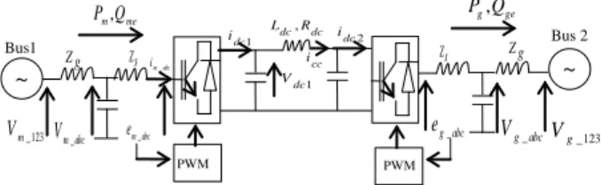
An HVDC system consists of three parts: a rectifier station, an inverter station and a high-voltage DC transmission line as shown in Fig. 1. Each converter is

connected to the AC network via a grid impedance Zg

representing the short-circuit power at the connection point.

Fig. 1. Two terminal HVDC-VSC link

For its advantage on control capability, the VSC technology is assumed. Each converter holds two degrees of freedom for the control. Usually, these degrees are used for the control of the reactive power at each side, of the active power and for the DC voltage [6]. Each station controls its reactive power independently of the other station. The flow of active power in the DC transmission system must be balanced, which means that the active power entering the HVDC system must mutch the active power leaving it, plus the losses in the DC transmission system. To achieve this power balance, one of the stations has to control the active power, while the other station should be designed for the DC voltage control. Usually, the two converters of an HVDC are controlled by two independent loops and each of these controls is based on the vector control approach in the d-q frame, using cascaded PI controllers [2]: the outer control loop generates the respective d-q current references to the inner current control loop.

III. SYNCHRONVERTER-BASED HVDC

In this section, a control strategy based on synchronverter technology is adapted for HVDC-VSC converters where the HVDC converters are run as synchronous machines. The synchronverter proposed in [9] is an inverter that mimics the structure and the regulations of a synchronous generator (SG). The usual control strategies used for conventional SG can thus be used for the inverter. For a complete DC system, a rectifier and an inverter are bound by a DC link. Therefore, to provide an HVDC structure, another synchronverter working as a synchronous motor (SM) based on the same mathematical derivation is necessary. As a result, the DC power is sent from the SM to the SG. Firstly, an overview of the synchronverter concept is presented, where the inverter is modeled according the mathematical model of a SG.

Next, the synchronverter concept is extended to a rectifier that mimics a SM.

A. Overview of the synchronverter concept

A synchronverter is an inverter which regulations are chosen such that the resulting closed-loop mimics the behavior of a conventional SG. For the purpose of the development, we recall the structure of a three phase round rotor synchronous machine [15] as shown in Fig. 2.

Fig. 2. Structure of an idealized three-phase round-rotor SG

The stator windings can be seen as concentrated coils having self-inductanceL and mutual inductance (- M ). The field winding can be seen as a concentrated coil having a

self-inductanceL .The phase terminal voltage vector f

_ [ ] T g abc ga gb gc V =V V V may be expressed by _ _ _ _ g abc

g abc s g abc s g abc

di V R i L e dt = − − + , (1) where _ [ ] T g abc ga gb gc

i = i i i is the stator phase currents

vector, Ls= +L M , R are, respectively, the inductance and s

the resistance of the stator windings. The back emf vector

_ [ ]

T g abc ga gb gc

e = e e e is the back emf given by

_

g abc g g g

e =M s

θ

sin

θ

, (2) where M is the flux field, g θgis the electric rotor angle and

( -2 ) ( +2 )

3 3

T g g g g

sinθ = sinθ sinθ π sinθ π _

 

 _{, (3)}

The mechanical equation of the machine is given by

g g gm ge gp g

J θ =T −T −D sθ , (4) where J is the combined moment of inertia of generator g and turbine, Tgmis the mechanical torque, T is the ge electromagnetic torque and Dgp is a damping factor. The

torque T is given by ge

Tge =Mg <ig_abc,sinθg >, (5)

where the operator < > denotes the conventional inner .,. product in ℝ3.

The real and reactive powers generated by the SG are, respectively _ , g g g g abc g P =M sθ <i sinθ >, (6) _ , ge g g g abc g Q = −M sθ <i cosθ >. (7) Based on the SG model above (Eq. 1-7), the concept of synchronverter is developed. The latter consists of an inverter on which specific controls are built and structured, as shown in Fig. 3. On the figure, we depict (i) the power

θg - + Rs, Ls a + Rf, Lf b Rs, Ls Rs, Ls c + + - - Vg_a Vg_b Vg_c - Zs _ m abc V Z g Z g Bus1 Bus 2 _ m abc e Zs _123 m V ~ , m me P Q P Qg, ge PWM PWM 1 dc V 2 dc i 1 dc i Ldc,Rdc _ g abc e _ g abc V V_{g_123} _ m abc i icc ~

part consisting of the inverter plus the LC filter and (ii) controls assured by the electronic part.

Such control structure is shown to be equivalent to a SG with capacitor bank connected in parallel with the stator terminal [9]. More specifically, with the terminal voltages

_

g abc

V and the voltages eg_abcdefined on the Fig. 3, the

voltage equation (1) holds. The voltage _ [ ]

T g abc ga gb gc

e = e e e

corresponds to the back emf of the virtual rotor. The inverter switches are operated so that the average values of

e

g a_ ,

_

g b

e

and

e

g c_ over a switching period are to be equal to eg_abc

given in (2). This can be achieved by the usual PWM technique. It’s worth noting that the VSC technology used in this work is not exclusive. However, it is suited for generating pulse control signals. The electronic part controls the switches in the power part. These two parts interact via the signals eg_abcandig_abc.

The synchronverter given in Fig. 3 is connected to the grid via the impedance (L ,g R ), thus, its output current and g voltage may be given by

_ _ _123 1 ( ) g abc g abc g f V i i C s = − , (8) _ 123 _ _ 123 1 ( ) ( ) g g abc g g g i V V R L s = − + . (9)

We may write a swing equation for the synchronverter, similar to equation (3): 1 ( ) g gm ge gp g g T T D s J θ = − − θ _,

where the mechanical torque Tgmis a control input,θg is the

angle position of the synchronverter. The electromagnetic torque T depends on ge ig_abcandθg.

To mimic the droop of the SG, the following frequency droop control loop is proposed

T_gm=T_gm__ref+D_gp(ω_n−sθ_g). (10) The synchronverter thus shares load with the other generators of the AC grid to which it is connected in proportion with the static droop coefficientDgp. In (10),

_ gm ref

T is the mechanical torque applied to the rotor and it is generated by a PI controller as shown in Fig. 3 to regulate the real power outputPg

_ _ ( _ )( _ ) g g i p gm ref p p g g ref K T K P P s = + − . (11)

The reactive power Qg is controlled by a voltage droop

control loop using a voltage droop coefficientDgq, in order

to regulate the field excitation Mg, which is proportional to

the voltage generated following (12) and (13)

1 ( ) g gm ge g M Q Q k s = − , (12)

Fig. 3. Model of the synchronverter: power and electronic parts [9]

g_ref ( _ ref )

gm gq g g

Q =Q +D V −V , (13)

where Vg is the output voltage amplitude computed by

2 3( g ga gb ga gc gb gc V V V V V V V = + + . (14)

B. Extension of the synchronverter concept to the HVDC emulation

To obtain an HVDC transmission system, in addition to a SG emulated by a synchronverter as in the section above, a rectifier that mimics a SM and a DC line are needed. The resulting system, a SM/SG and a DC line are called Synchronverter High-Voltage Direct Current (SHVDC). B.1. The synchronverter model of a SM

The synchronverter model of a SM consists of an LC filter and mainly controls shown in the same Fig. 3. It’s nearly the same model discussed above, apart from the fact that the sign

convention for the stator current _ [ ]

T m abc ma mb mc

i = i i i is

changed. Equations (1), (4), (8) and (9) are re-written in motor convention

_

_ _ _

m abc m abc s m abc s m abc

di V R i L e dt = + + , (15) 1 ( ) m me mm mp m m T T D J θ = − − θ _{, (16)} _ _ 123 _ 1 ( ) m abc m m abc f V i i C s = − _{, (17)} _ 123 _ 123 _ 1 ( ) ( ) m m m abc g g i V V R L s = − + . (18)

The bloc equations (2), (5) and (7) remain the same

_ sin m abc m m m e =M sθ  θ , (19) _ , me m m abc m T =M <i sinθ > , (20) _ , me m m m abc m Q =M s

θ

<i cos

θ

> , (21) _ , m m m m abc m P =M sθ <i sinθ >. (22) The frequency and the voltage droop controls are also similar to the SG emulation case; except for the power regulation (11) which is replaced by the DC voltage control loop as defined by (24) ~ _ g ref V _123 g i _ g ref P g M − ge T − n ω g θ θg 1 J *s g gp D (2) (4) (5) Eqn Eqn Eqn 1 k s_g _ gm ref T (11) Eqn 1 s _ e g abc g V (14) Eqn _ g abc i _ g abc e Bus 2 , s s R L ~ , g ge P Q ge Q − − cc i idc2 2 dc V − f C _123 V g _ i g abc g P gq D _ g ref Q dc C PWM _ V_{g abc} , g g R L

_ ( ) mm mm ref mp n m T =T +D ω −sθ , (23) _ _ _ 1 _ ( i vdc)( ) mm ref p vdc dc ref dc K T K V V s = + − , (24) m_ref ( _ ) mm mq m ref m Q =Q +D V −V , (25) 1 ( ) m mm me m M Q Q k s − = − , (26) 2 3( m ma mb ma mc mb mc V V V V V V V = + + . (27) B.2. Coupling equations

The circuit equations of the DC line (Fig. 1 & 3) are

1 1 1 ( ) dc dc cc dc V i i C s = − , (28) 2 2 1 ( ) dc cc dc dc V i i C s = − , (29) 1 2 1 ( ) cc dc dc dc cc dc i V V R i L s = − − . (30)

The AC and DC circuits are coupled by the active power relation 1 1 1 dc dc dc P =V i , (31) 2 2 2 dc dc dc P =V i , (32) 1 dc m P =P , (33) 2 dc g P =P . (34) IV. STRUCTURAL ANALYSIS OF SYNCHRONVERTERS BASED

HVDC

In this section, the SHVDC is analyzed from a structural point of view. More precisely, the droop and voltage regulations introduced in [9] for the synchronverter in Fig. 3 are appropriate in the sense that they cancel all the degrees of freedom of the system, so that, with given initial conditions, the trajectories of the closed-loop system in Fig. 3 are uniquely defined. Roughly speaking, the number and the nature of the regulations are necessary and sufficient for this system. When coupling two synchronverters as in Section II to form the SHVDC, this fact is not obvious. Moreover, controls for the power exchange and the DC voltage have been added by equations (11) and respectively (24). The scope of this section is to prove that the proposed structure is well-defined from the point of view mentioned above. As the model of the SHVDC is given by equations (1)-(34) in a general Differential Algebraic Equations (DAE) form, the approach introduced in [17] and related references can be directly used. In this latter, a linear systemΣ is a module M

defined by a matrix equation

( ) 0

S s w = , (35)

where S s( )is a matrix which elements are polynomials in the derivation operator s=d dt. For the SHVDC, w is given by (36), and S s( )results from the linear approximation of equations (1)-(34). Let k= length (w) and r=rank (S(s)).

g_abc g_abc g_abc g_123 m_abc m_abc m_abc m_123 g

ge gm gm_ref g m me mm mm_ref m ge gm g g T dc1 dc1 dc1 me mm m m dc2 dc2 cc dc2 w=[i ,V ,e ,i ,i ,V ,e ,i ,P , T ,T ,T ,θ ,P ,T ,T ,T ,θ ,Q ,Q ,M ,V , V ,i ,P ,Q ,Q ,M ,V ,V ,i ,i ,P ,sin θ_g] . (36)

From [17], the integer k =m−ris the rank of the moduleM

, which coincides with the rank of the linear systemΣ . The number of the independent inputs u={u1...um}of the

system M given by (35) is the rank of the module which

defines the system m=rank (M). For the SHVDC case, the rank of the module M defined by the SHVDC is zero, which means that the regulations included in (1)-(34) are necessary and sufficient to well define the behavior of this structure. The choice of the regulations parameters in order to ensure stability and desired performances is next discussed.

V. TUNING OF ASYNCHRONVERTER BASED HVDC

The SHVDC structure is investigated in this section on the simple system of Fig. 1. A four machines system will be used in Section VI. The simulations tool in the Matlab/Simulink toolbox.

A. Tuning with standard parameters of classic SG

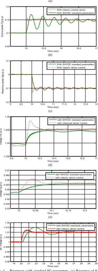
The main advantage of the synchronverter is to put into evidence the structure of classic generators for which the controls are well known. For this reason, we firstly adopted for the new SHVDC structure standard parameters of a SG which are given in the first column of Table III. They mainly correspond to 5% governor droop [15] (1 Dgpand 1 Dmp) and a 3% AVR gain (1 Dgq and 1 Dmq) [18]. The responses of the SHVDC to step changes in active/reactive power references are given in Fig. 4 in solid lines in comparison with the ones in dotted lines obtained with a classic vector control (see, e.g., [19]). Although the voltage and reactive power dynamics are quite similar, a poorly damped response is obtained for the active power P with the SHVDC. As a consequence, the usual parameters of a synchronous generator of the same capacity cannot be directly used for the SHVDC and a specific tuning of the parameters of the latter was done as presented in the next section.

B. Specific framework for the tuning of the SHVDC parameters

B.1. HVDC control specifications: we first recall the usual full set of control specifications for a VSC based HVDC, as presented in Section II. Set-points for the transmitted active power, the reactive power and the voltage at the points of coupling have to be tracked with the following transient performances [6, 20]:

-the response time of the active/reactive power is normally in the range of 50 ms to 150 ms.

- the response time for voltage is about 100 ms to 500 ms. The dynamic of the HVDC should also improve the stability of the neighboring (see, e.g., [5]).

(a)

(b)

(c)

(d)

(e)

Fig. 4. Responses with standard SG parameters. (a) Response ofPgto a

+0.05 step in Pg_ref (p.u) ; (b) Response of Qgto a -0.1 step in Qg_ref (p.u);

(c) Response of Vgto a −0.1 step change in Qg_ref (p.u); (d) Response of

m

V to a −0.1 step change in Qm_ref (p.u); (e) Response of Vdc to a +0.01

step in Vdc_ref (p.u).

B.2. Control structure: in order to satisfy these specifications, the SHVDC parameters should be tuned simultaneously and in a coordinated way. For this tuning, the SHVDC shown in Fig. 1 is put into the feedback system structure presented in Fig. 5 where∑is modeled by equations (1) to (34) with the exception of equations (10), (11), (13), (24), (25) and (26). All control parameters are grouped in the following diagonal matrix

g g

gp mp p_Vdc i Vdc gq mq p_p i p

K(s,q)=diag(D ,D ,K ,K _ ,D ,D , K ,K _ ) . (37)

Fig. 5. Feedback system

where D_gp, D_mp are, respectively, the static frequency droop

coefficients of the SG and the SM; D_gq,D_mqare,

respectively, the voltage droop coefficient of the SG and of the SM; Kp V_dc,Ki V_dcare the DC voltage PI control

parameters; and Kp P_g , Ki P_gare the active power PI control

parameters.

Note that all elements of the matrix K s q are tuned via the ( , ) pole placement presented in Section V.B.3 to meet HVDC performance specifications given in Section V.B.1.

The inputs u and the outputs y are

mm mm mm ref_kp mm ref_ki gm gm gm ref_kp

T gm ref_ki u=[T ,Q ,T _ ,T _ , T ,Q ,T _ , T _ ] dc_ref dc m m_ref m dc_ref dc g g_ref g g_ref g g_ref g V V y=[ -sθ , V V , V V , , -sθ , s P P V V , P P , ] . s n n T ω − − − ω − − −

B.3. Regulator parameters and residues: letH s( )be the transfer matrix of a linear approximation of∑and consider each closed-loop of the feedback system in Fig. 5 which corresponds only to input uiand outputyi

Fig. 6. Single input/Single output feedback system

More specifically,H_ii( )s andK_ii( )s are the (i,i) transfer functions of H(s), K s q( , ), respectively.

Proposition (e.g., [21]): The sensitivity of a poleλ of the

closed-loop in Fig. 6 with respect to a parameter qof the

regulator Kii is ( , ) ii K s q r q λ q λ ∂ ₌ ∂ ∂ ∂ (38)

where r_λis the residue of H_ii( )s at poleλ .

15 15.5 16 16.5 17 0.65 0.7 0.75 0.8 Time (sec) A c ti v e pow er P g ( p. u)

With classic control vector With SHVDC standard parameters

9 9.5 10 10.5 11 11.5 12 12.5 13 -0.2 -0.1 0 0.1 Time (sec) R eac ti v e pow er Q g ( p. u)

With SHVDC standard parameters With classic vector control

9.8 10 10.2 10.4 10.6 10.8 11 1.035 1.04 1.045 1.05 Time (sec) V ol tage V m ( p. u)

with SHVDC standard parameters with classical vector control

10 10.05 10.1 10.15 10.2 0.93 0.935 0.94 0.945 0.95 0.955 0.96 0.965 0.97 Time (sec) V ol tage V g ( p. u)

with SHVDC standard parameters with classic vector control

19 20 21 22 23 24 25 26 27 28 29 30 0.98 0.985 0.99 0.995 1 1.005 1.01 1.015 1.02 Time( sec) D C V ol tage ( p. u)

with SHVDC stantards parameters with classic vector control

∑ ( , ) K s q ' u +

e

y

u

( ) ii H s ( , ) ii K s q + i e ui ' yi i u

Note that, for our case. (37), ii( , ) 1 s K s q q _=λ ∂ ₌ ∂ .

Also, the poles of Hii( )s are among the poles ofH s( ). As a

consequence, the residues of the linear approximation of ∑ can be used for the pole placement as shown in Section V.D. Before, some basic notions of modal analysis are recalled. C. Modal analysis of the system

This analysis is based on a state representation of the transfer matrix H s( ) of the form

: x=A x+B , =C xu y

Σ  . (39)

The poles λ of i H s( )correspond to the eigenvalues (modes)

of A. The participation factors measure the relative participation of the kth state variable in the ith mode:

*

ki ik ki

p =ψ ϕ , (40) where ϕi and ψi are respectively the right and the left

eigenvectors ofA associated with the modeλ . They are given i

in Table II for system (39).

Each element H sij( ) of H s( ) can be expanded in partial fractions

as 1 ( ) k n k ij k k r H s s λ = = = −

∑

, (41) where rk is the residue of H sij( ) at pole λ expressed as i

k i k k j

r =C ϕ ψ B , (42) where Ci is the i

th

line of C and Bj is the j

th

column of B [21]. D. Coordinated tuning of SHVDC parameters

First, desired locations *

i

λ can be computed for each pole

i

λ starting from the control specifications given in Section B.1. To ensure a second order type response without overshoot, the damping of the corresponding complex mode λi is imposed to

beζ_i =0.7. The frequency of the mode is deduced from the desired response time tr given in Section B.1: ωi0=3tr [21].

Thus, the desired location ofλiis

* 2

0 0 1

i i i j i i

λ = −ζ ω ± ω −ζ and the results for the dynamics of interest for the SHVDC are given in Table I (column 3).

It should be noted that, the dynamic of reactive power is the same as the dynamic of the voltage. The connections in Table I between the dynamics of interest and the modes are established based on the participations factors given in Table II. Only the highest participation factor is considered, therefore each dynamic is associated to only one pole for the

computation of desired poles *

i

λ . However, from the same

column of Table II; several poles have also significant participations to the same dynamic which led us to compute the gainsK in a coordinated way. More specifically, ifΛ denotes the set indices j from 1 to 8 for which Hjj( )s hasλias pole, the contribution of each control gain in the shift of the pole is 0 i i ij j j r K λ λ ∈Λ = +

∑

, (43) where 0 i

λ is the initial (open-loop) location of the poleλiand

ij

r is the residue of Hjj( )s in λi. Finally, the pole placement is the solution of the following optimization problem

2 * * { , 1...8} arg min j j i i K i K j= =

∑

λ −λ , (44) where λiis given by (43). TABLE I

DESIRED MODES MEETING THE HVDC SPECIFICATIONS

TABLE II PARTICIPATION FACTORS

TABLE III SHVDC PARAMETERS

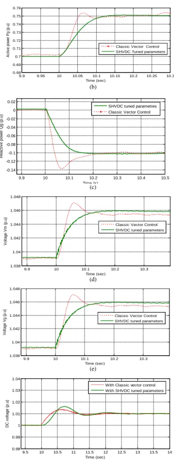
The optimal parameters in the second column of Table III were obtained with (44) solved for the desired locations in Table I. The response of SHVDC for the link in Fig. 1 with these tuned parameters is given in Fig. 7 in solid lines in comparison with the ones in dotted lines obtained with a classic vector control. The active power, the voltage and the reactive power dynamics are similar which prove that the performances given in Section B.1 are correctly ensured by the proposed control methodology. Notice, however, that less overshoots with the new tuned parameters are obtained. The robustness of this approach is studied in the next section on a four machines case.

(a) Dynamics of interest 0 i λ * i λ 0 i r_λ Voltage Vm -3.8713 -10 -0.543 Voltage V g 3.537 -10 -0.65

Active Power P m 1.8± 5.89i -21±21.42i -0.06 ±0.01i

Active Power P g -3.3±10.3i -21±21.42i -0.06 ± 0.1i

Reactive Power Q m -3.8713 -10 -0.543 Reactive Power Q g 3.537 -10 -0.65 % _ m/ m a V Q P Pa V_ g/Qg Pa_Pm Pa_Pg 0 / m m V Q λ 57 2.1 21.8 28 0 m P λ 0.2 71.9 0.3 15.8 0 / g g V Q λ 21.7 7.6 40 2.2 0 g P λ 1.8 14 1.7 42.8 K SHVDC standard parameters SHVDC optimal parameters mp D 20 94.82 mq D 33.33 50.24 _dc p V K 5 15.149 __dc i V K 2 16.501 gp D 20 92.843 gq D 33.33 57.20 _g p P K 5 27.61 __g i P K 3 12.62

(b)

(c)

(d)

(e)

Fig. 7. Responses with optimal parameters. (a) Response ofPgto a +0.05

step in Pg_ref (p.u) ; (b) Response of Qgto a -0.1 step in Qg_ref (p.u); (c)

Response of Vgto a −0.1 step change in Qg_ref (p.u); (d) Response of V to m

−0.1 step change in Qm_ref (p.u); (e) Response of Vdc to a +0.01 step in

_

dc ref

V (p.u).

Fig. 8. Two area test system with parallel AC and DC lines

VI. FOUR MACHINES TEST POWER SYSTEM

In this section, the specific tuning SHVDC parameters presented in Section V is tested and compared with the classic vector control on the IEEE 4 machines benchmark [15] shown in Fig. 8. The two areas are connected with an AC line in parallel with one HVDC link. The 150 km HVDC cable link has a rated power of 200 MW and a DC voltage rating of ±100 kV. Each area consists of two identical generating units of 400 MVA/20 kV rating. Each of the units is connected through transformers to the 100 kV transmission line. There is a power transfer of 400 MW from Area 1 to Area 2. The detailed system data is given in the appendix. The loads L1 and L2 are modeled as constant

impedances.

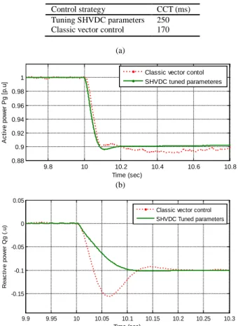
The control SHVDC approach is assessed for local performances and for transient stability. The desired HVDC performances given in Section V are fulfilled as shown by the step responses in Fig. 9. As for the case of the two-machine system, responses with less overshoot are obtained compared to the vector control approach.

Fig. 10 shows the response of the angular speed of generator G1 to a three phase short circuit fault of 100 ms duration, occurring in the mid-point of the AC transmission line. We can depict a better dynamic performance with the proposed controller: the transient oscillations with the SHVDC control are more damped. For the same fault, transient stability is assessed by the Critical Clearing Time (CCT), which is the maximum time duration that a short-circuit may act without losing the system capacity to recover to a steady-state (stable) operation.

The obtained CCTs for a three-phase short-circuit fault in the mid-point of the AC transmission line are presented in Table IV for the classic vector control, and the proposed SHVDC control. We can see that the SHVDC control with tuned parameters improves the transient dynamics of the system and thus augments the transient stability margins of

the neighbor network. This is due to the fact that the

dynamics of the neighbour zone are taken into account at the synthesis stage via the oscillatory modes in Table I. The gains of the controllers are computed to damp these modes and thus to diminish the general swing of the zone and not only for the local HVDC dynamics. Moreover, as the structure of the SHVDC mimics the closed-loop of a standard synchronous generator, an inertia with a positive impact of the transient stability of the neighbour zone is emulated. 9.9 9.95 10 10.05 10.1 10.15 10.2 10.25 10.3 0.68 0.69 0.7 0.71 0.72 0.73 0.74 0.75 0.76 Time (sec) A ct iv e pow er P g ( p. u)

Classic Vector Control SHVDC Tuned parameters 9.9 10 10.1 10.2 10.3 10.4 10.5 -0.14 -0.12 -0.1 -0.08 -0.06 -0.04 -0.02 0 0.02 Time (s) R eac ti v e pow er Q g ( p. u) SHVDC tuned parametres Classic Vector Control

9.9 10 10.1 10.2 10.3 1.038 1.04 1.042 1.044 1.046 1.048 Time (sec) V ol tage V m ( p. u)

Classic Vector Control SHVDC tuned parameters 9.9 10 10.1 10.2 10.3 1.038 1.04 1.042 1.044 1.046 1.048 Time (sec) V ol tage V g ( p. u)

Classic Vector Control SHVDC tuned parameters 9.5 10 10.5 11 11.5 12 12.5 13 13.5 14 0.98 0.99 1 1.01 1.02 1.03 1.04 Time (sec) D C v ol tage ( p. u)

With Classic vector control With SHVDC tuned parameters

G4 G3 400 MW 1 2 3 5 4 6 7 8 25 km 9 10 km 10 km 25 km 10 L1 L2 200 km Area 1 Area 2 G1 G2 ~ ~ ~ ~

TABLE IV

CRITICAL CLEARING TIMES WITH BOTH CONTROL STRATEGIES

(a)

(b)

Fig. 9. Responses of the IEEE 4 machines benchmark. (a) Response of Pg to a -0.1 step in Pg_ref (p.u) ; (b) Response of Qg to a -0.1 step in Qg_ref (p.u).

Fig. 10. Speed response of G1 to a 100 ms short-circuit

Remark: Real-time implementation

The SHVDC system is based on the Sinusoidal Pulse Width Modulation (SPWM) switching using a single-phase triangular carrier wave with a frequency of 27 times fundamental frequency (1350 Hz). This is compliant with the real time implementation which relies on a time response of 1-3 µs [22]. Indeed, in the real time simulation, the converter stations and the connecting DC cable are simulated in three separate small time step networks [23]. The three subnetworks are connected on the DC side through travelling wave transmission line models with a travel time in the range of the small time step size (i.e. ~3µs). Both converter stations are interfaced to the AC systems with the help of interfacing transformers connecting the small and the normal time step areas.

VII. CONCLUSION

This paper proposed a new control strategy of HVDC transmission based on the synchronverter concept. The proposed synchronverter structure could not be controlled using directly the standard parameters of the SG. Thus, a specific tuning method was proposed based on; firstly, the sensitivity analysis of the system poles to the control parameters then, their placement linear approximation via residues. Better results than with the classic VSC control were obtained for the following points:

- Better dynamic performances (less overshoot and more damping) because this approach allows one to analytically take into account dynamic specifications at the tuning stage. - Better stability margin of the neighbor zone for two reasons. First, swing information is directly taken into account at the synthesis stage in terms of the less damped modes of the neighbor zone and not only for the local HVDC dynamics as it is the case for the standard VSC control. Next, the SHVDC emulates inertia of two rotating machines and this has a direct damping effect for the neighbor zone.

- Help power system operators in system operation since the SG and their controls are better known.

It is noted that this kind of tuning is surely under optimal in the sense that the constraints to keep the structure of the classical generators and their regulations imposed by the synchronverter principle limits the performances of the resulting closed-loop. Moreover, the advantage of inertia emulation mentioned above could be lost in the context of a grid with many power electronics and few physical SG since the grid frequency is no longer (well) defined in this case.

VIII. REFERENCES

[1] D. Murali, M. Rajaram, and N. Reka, "Comparison of FACTS Devices for Power System Stability Enhancement," International Journal of Computer Applications (0975– 8887), 2010, Volume 8– No.4.

[2] F. Wang, L. Bertling, and T. Le, "An Overview Introduction of VSC-HVDC: State-of-art and Potential Applications in Electric Power Systems," Cigré 2011.

[3] F. Goodrich, and B. Andersen, "The 2000 MW HVDC link between England and France," Power Eng. J., 1987, 1, (2), pp. 69–74. [4] Y. Decoeur, "France-Spain interconnections, First step for smart grids ",

inelfe, Madrid, March 26th, 2012.

[5] A.E. Hammad, J. Gagnon and D. McCallum, "Improving the dynamic performance of a complex AC/DC system by HVDC control modifications," IEEE Trans. Power Delivery, 1990, 5, (4), pp. 1934– 1943.

[6] S. Li, T.A. Haskew, and L. Xu, , "Control of HVDC light system using conventional and direct current vector control approaches," IEEE Trans. Power Electr., 2010, 25, (12), pp. 3106–3118.

[7] H. Latorre, and M. Ghandhari, "Improvement of power system stability by using a VSC-HVDC, "Int. J. Electr. Power Energy Syst, 2011, 33, (2), pp. 332–339.

[8] N. Rostamkolai, A.G. Phadke, W.F. Long, and J.S. Thorp, "An adaptative optimal control strategy for dynamic stability enhacement of AC/DC power systems, " IEEE Trans. Power Syst., 1988, 3, (3), pp. 1139–1145.

[9] Q.-C. Zhong, and G.Weiss, "Synchronverters: Inverters that mimic synchronous generators," IEEE Trans. Ind. Electron., Apr. 2011, vol. 58, no. 4, pp. 1259–1267.

[10] L. Zhang, L. Harnefors, and H.-P. Nee, "Power synchronization control of grid-connected voltage-source converters," IEEE Trans. Power Syst, May 2010, vol. 25, no. 2, pp. 809–820.

[11] H.-P. Beck, and R. Hesse, "Virtual synchronous machine, " in Proc. of the 9th International Conference on Electrical Power Quality and Utilisation (EPQU), 2007, pp. 1–6. 9.8 10 10.2 10.4 10.6 10.8 0.88 0.9 0.92 0.94 0.96 0.98 1 Time (sec) A c ti v e pow er P g [ p. u]

Classic vector contol SHVDC tuned parameteres 9.9 9.95 10 10.05 10.1 10.15 10.2 10.25 10.3 -0.15 -0.1 -0.05 0 0.05 Time (sec) R eac ti v e pow er Q g ( .u)

Classic vector control SHVDC Tuned parameters 9 10 11 12 13 14 15 0.99 0.995 1 1.005 1.01 Time (sec) A ngul ar s peed of G 1 ( p. u)

with classic vector control with tuned SHVDC parameters

Control strategy CCT (ms) Tuning SHVDC parameters 250 Classic vector control 170

[12] J. Driesen, and K. Visscher, "Virtual synchronous generators," in Proc. of IEEE Power and Energy Society General Meeting, 2008, pp. 1–3. [13] Y. Chen, R. Hesse, D. Turschner, and H.-P. Beck, "Improving the grid

power quality using virtual synchronous machines," in 2011 International Conference on Power Engineering, Energy and Electrical Drives (POWERENG), 2011, pp. 1–6.

[14] M. Torres, and L. A. C. Lopes, "Frequency control improvement in an autonomous power system: An application of virtual synchronous machines," in 2011 IEEE 8th _{International Conference on Power} Electronics and ECCE Asia (ICPE & ECCE), 2011, pp. 2188–2195. [15] P. Kundur, "Power system stability and control", Mc Graw-HillInc,

1994.

[16] P-L. Nguyen, Q-C. Zhong, F. Blaabjerg, and J-M. Guerrero, " Synchronverter-based Operation of STATCOM to Mimic Synchronous Condensers", 2012 7th IEEE Conference on Industrial Electronics and Applications (ICIEA).

[17] H. Bourlès, and B. Marinescu, "Linear-Time Varying Systems, Algebraic-Analytic Approach", Springer-Verlag, LNCIES 410, 2011. [18] IEEE Recommended Practice for Excitation System Models for Power

System Stability Studies, IEEE Power Engineering Society, 21 April 2006.

[19] S. Li, T.A. Haskew, L. Xu, "Control of HVDC light system using conventional and direct current vector control approaches", IEEE Trans. Power Electr., 2010, 25, (12), pp. 3106–3118.

[20] M-K-S. Sangathan, J- Nehru "Performance of high-voltage direct Current (HVDC) systems with Line-commutated converters", bureau of find Indian standard Manak Bhavan, 9 Bahadur Shah Zafar Marg New Delhi 110002 , April 2013.

[21] G. Rogers, "Power System Oscillations", Kluwer Academic, 2000. [22] P.A. Forsyth, T.L. Maguire, D. Shearer, D. Rydmell, ‘’ Testing Firing

Pulse Controls for a VSC Based HVDC Scheme with a Real Time Timestep < 3 µs’’, the International Conference on Power Systems Transients (IPST2009) in Kyoto, Japan June 3-6, 2009.

[23] Pinaki Mitra, Vinothkumar K , Lidong Zhang, ‘’ Dynamic Performance Study of a HVDC Grid Using Real-Time Digital Simulator’’, IEEE Workshop on Complexity in Engineering 11 June, Aachen, Germany 2012.

IX. APPENDIX

Network data (Fig. 1)

Bus system 1 & 2: line voltage=100 kV, frequency=50 Hz, Short circuit power=600 MVA, Rs=0.75Ω , Ls=0.2 H

27th AC filter in AC system 1 & 2: reactive power=18 MVAR, tuning frequency=1620 Hz, quality factor=15.

54th AC filter in AC system 1 & 2: reactive power=22 MVAR, tuning frequency=3240 Hz, quality factor=15.

DC system: voltage= ±100 kV, rated DC power=200 MW, Pi line R=0.0139 Ω /km, L=159 µH/km, C=0.331 µF/km, Pi line length= 150 km, switching frequency=1620 Hz, DC capacitor=70 µF, smoothing reactor: R=0.0251Ω , L= 8mH.

Parameters of the classic vector control: current loop: kp=0.6, ki=6, reactive power control: ki=20, active power control: ki=20, DC voltage control: kp=5, ki=2.

Network data (Fig. 8)

Generators: Rated 400 MVA, 20 kV Xl (p.u): leakage Reactance = 0.18

Xd (p.u.): d-axis synchronous reactance = 1.305, T’d0 (s): d-axis open circuit sub-transient time constant =0.296, T’d0 (s): d-axis open circuit transient time constant = 1.01

Xq (p.u): q-axis synchronous reactance = 0.053, Xq (p.u): q-axis synchronous reactance = 0.474, X’’q (p.u): q-axis sub-transient reactance =0.243, T’’q0 (s): q-axis open circuit sub transient time constant=0.1

M =2H (s): Mechanical starting time = 6.4 Governor control system

R (%): permanent droop =5, servo-motor: ka = 10/3, ta (s) = 0.07, regulation PID: kp = 1.163, ki= 0.105, kd= 0

Excitation control system

Amplifier gain: ka = 200, amplifier time constant: Ta (s) = 0.001, damping filter gain kf = 0.001, time constant te (s) = 0.1

27th AC filter in AC system 1 & 2: reactive power=18 MVAR, tuning frequency=1620 Hz, quality factor=15.

54th AC filter in AC system 1 & 2: reactive power=22 MVAR, tuning frequency=3240 Hz, quality factor=15.

DC system: voltage= ±100 kV, rated DC power=200 MW, Pi line R=0.0139 Ω /km, L=159 µH/km, C=0.331 µF/km, Pi line length= 150 km, switching frequency=1620 Hz, DC capacitor=70 µF, smoothing reactor: R=0.0251Ω , L= 8mH.

Generator transformers Rated 400 MVA, 20/ 100 kV Coupling Delta/ Yg

Primary resistance (p.u) =0.002, Primary inductance (p.u) =0.12 Secondary resistance (p.u) =0.002, Secondary inductance (p.u) =0.12 Loads: PL1=200 MW, PL2= 1GW

AC transmission lines

Resistance per phase (Ω/km) =0.03 Inductance per phase (mH/km) =0.32 Capacitance per phase (nF/km) =11.5

Parameters of the classic vector control: current loop: kp=0.6, ki=8, reactive power control: ki=40, active power control: ki=40, DC voltage control: kp=1, ki=10.