HAL Id: hal-01147369
https://hal.archives-ouvertes.fr/hal-01147369
Submitted on 7 Jul 2015
HAL is a multi-disciplinary open access archive for the deposit and dissemination of sci-entific research documents, whether they are pub-lished or not. The documents may come from teaching and research institutions in France or
L’archive ouverte pluridisciplinaire HAL, est destinée au dépôt et à la diffusion de documents scientifiques de niveau recherche, publiés ou non, émanant des établissements d’enseignement et de recherche français ou étrangers, des laboratoires
Energy Storage Control with Aging Limitation
Pierre Haessig, Hamid Ben Ahmed, Bernard Multon
To cite this version:
Pierre Haessig, Hamid Ben Ahmed, Bernard Multon. Energy Storage Control with Aging Limi-tation. PowerTech 2015, IEEE, Jun 2015, Eindhoven, Netherlands. �10.1109/PTC.2015.7232683�. �hal-01147369�
Copyright notice: this article has been accepted to the PowerTech 2015 conference (http:// powertech2015-eindhoven.tue.nl). Copyright may be transferred without notice to IEEE.
Energy Storage Control with Aging Limitation
Pierre Haessig
∗, Hamid Ben Ahmed, Bernard Multon
†Abstract
Energy Storage Systems (ESS) are often proposed to mitigate the fluctuations of renewable power sources like wind turbines. In such a context, the main objec-tive for the ESS control (its energy management) is to maximize the performance of the mitigation scheme.
However, most ESS, and electrochemical batteries in particular, can only perform a limited number of charge/discharge cycles over their lifetime. This limi-tation is rarely taken into account in the optimization of the energy management, because of the lack of an appropriate formalization of cycling aging.
We present a method to explicitly embed a limita-tion of cycling aging, as a constraint, in the control op-timization. We model cycling aging with the usual “ex-changed energy” counting method. We demonstrate the effectiveness of our aging-constrained energy manage-ment using a publicly available wind power time series. Day-ahead forecast error is minimized while keeping storage cycling just under an acceptable target level.
1 Introduction to Aging Control
1.1 Why Limiting Aging in Energy Storage Control?
Energy Storage Systems (ESS) like electrochemical batteries can be used as buffers to reduce power fluc-tuations in different applications. For wind or solar power generation, an ESS can mitigate the fluctua-tions of the renewable power source. In an hybrid electric vehicle (HEV), it absorbs the fast fluctuations of the driving power profile to keep the combustion engine close to an efficient operating point.
∗P. Haessig is with IETR, CentraleSup´elec, Rennes, France. This
work was partly conducted while he was at ENS Rennes, sponsored by EDF R&D.
†H. Ben Ahmed, B. Multon are with SATIE lab, ENS Rennes,
Bruz, France
In these two applications, the control of the ESS is often treated as an optimization problem where the objective is to maximize the performance of the overall system. Performance criterions can be, for example, the fuel efficiency for a HEV, or a mea-sure of the fluctuations at the output of a combined wind-storage system (cf. figure 1 introduced in the next section). The control decides how and when to charge and discharge the battery to maximize the performance objective.
However, most ESS, and electrochemical batteries in particular, can only perform a limited number of charge/discharge cycles over their lifetime. This ag-ing phenomenon causes a degradation of the battery parameters: decrease of the capacity, increase of the series resistance. This can lead to an eventual ESS re-placement. This is why aging is crucial for evaluating and then minimizing the life-cycle cost of an ESS [1,2]. Unfortunately, battery aging is seldom taken di-rectly in the control optimization. Often, it is only after simulating the behavior of the system, that an aging study is conducted. Before discussing existing work on aging control, we need to give an overview of aging modeling.
1.2 Models for Cycling Aging
The purpose of limiting battery aging requires a model for the aging phenomenon. Battery aging can be studied at the microscopic scale of the degradation processes, which is a research field by itself. How-ever, for control, we need simpler models that are defined on the system level. Our work relies on ag-ing models from the literature which are well in line with the datasheets provided by battery manufactur-ers. The verification of such models using (acceler-ated) aging test benches is again another field of ex-pertise.
ag-ing is the “Ah throughput” model. It is widely de-scribed in the literature [3, §4] [4, §4], with some vari-ations like “weighted Ah throughput” models to ac-count for technology-specific aggravating aging fac-tors.
This model considers that a battery can exchange a fixed amount of charge over its life. As such, the model consists in integrating over time the cur-rent that goes in and out of the battery (thus the name “Ah-throughput”). We use a common variation which consists in counting the exchanged energy in-stead of the charge (Wh vs. Ah). This energy counting model integrates the absolute power Psto of the
bat-tery:
Eexch(t ) =
Z t
0 |Psto|dt (1)
and this exchanged energy is then compared with the energy exchanged during one full charge-discharge cycle, i.e. two times the energetic capacity of the bat-tery (2Er ated). The ratio gives Ncycl, the number of
equivalent full cycles:
Ncycl(t ) = Eexch(t )/(2Er ated) (2)
This number increases with time, and when it reaches Nlif e, the maximum number of full
charge-discharge cycles, the battery is considered to be in end-of-life and should be replaced1. Nlif e is
typi-cally between 500 and 5000 for batteries. An impor-tant property of this counting method is that it al-lows a number of cycles that is inversely proportional to the amplitude of these cycles (often called Depth of Discharge). This fact is often verified on the “aging curves” provided by manufacturers of lead-acid bat-teries. The reader can find a deeper analysis on the link between energy counting and cycle counting in Serrao et al. [5] and our thesis [6, §2.2].
Now that an aging model is established, we can turn to our main contribution: the mitigation of cy-cling aging through the ESS control.
1.3 Previous Work on Aging Control
The problem we have described in section 1.1 was already underlined by some authors [7–9]. We can summarize some keys aspects of their contributions: Serrao et. al [7] (HEV context) and Borhan et. al
1A common and equivalent expression is to define a State of
Aging (SoA) as the Ncycl(t ))/Nlif eratio. SoA starts at 0 zero,
and end-of-life is reached when SoA(t) = 1
[8] (wind power context) both use weighted charge counting to model cycling aging, while Koller et. al [9] (peak shaving context) use a piece-wise affine model with quadratic cost because it enables efficient optimization solving.
All these approaches attempt to reduce the aging by adding the aging increase as a penalty in the opti-mization criterion, which otherwise contains only a performance criterion (like the HEV fuel efficiency). The control designer is thus forced to tune a weight-ing factorto find a satisfactory compromise between performance and aging.
We propose instead to express aging limitation as an inequality constraint rather than a cost penalty. This can ease the implementation of aging limitation, because the control designer can directly set a desired maximum number of cycles Nlif e, with no need for
tuning.
1.4 Reformulating aging limitation as a constraint
Based on the cycle counting model (2), we can indeed express aging limitation as an inequality constraint. Given Tlif e, the expected lifetime of the project
in-volving the ESS, the non replacement of the stor-age during the operational period is expressed by Ncycl(Tlif e) ≤ Nlif e. This translates into a constraint
on the mean absolute storage power: 1
Tlif e
Z Tl i f e
0 |Psto|dt = h|Psto|iTl i f e ≤Pexch (3)
where Pexch is what we call the mean exchangeable
power. It is the ratio of the lifetime exchangeable en-ergy of the storage with the duration of the project:
Pexch = 2Er atedNcycl/Tlif e (4)
Inequality (3) is the condition that should be sat-isfied by the ESS control algorithm (which sets Psto
at each time) to limit the aging. However, this is an integral constraint on a very long time horizon (Tlif e
typically in the range of 5 to 20 years). This horizon is much longer than a usual ESS control horizon (on the order of the energy/power ratio of the ESS, i.e. minutes to hours). It cannot be practically solved by common control algorithms such as Model Predictive Control (MPC) or Stochastic Dynamic Programming (SDP). As such, expressing the lifetime constraint (3)
Storage Control
to fulfill a production commitment
Storage Production Grid Storage Energy Control Commitment Forecasting Payoff & Penalty
Figure 1: Wind-storage system used as a context for storage aging limitation
is only a first step, and our key contribution is to re-place lifetime constraint (3) with a manageable con-straint, in the next section.
2 Problem Description
2.1 Modeling
2.1.1 Wind-storage system
We base our study on the context of a wind-storage system for a day-ahead production commitment. The storage is used to mitigate the fluctuations of the wind power plant (see [10, 11] for previous work on this context). Figure 1 shows the variable and energy flows of this system, with the three main ones high-lighted in red:
• Pmis is the difference between the wind power
production Pprod and the commitment Pдr id∗
made one day in advance, based on a produc-tion forecast2.
• Psto is the power absorbed by the storage
(con-vention Psto > 0 when charging, Psto < 0 when
discharging).
• Pdevis the commitment deviation (Pдr id−Pдr id∗ )
for which the wind operator must pay penalties to the grid operator (cf. [10] for detailed con-text).
The commitment deviation can be written as:
Pdev = Pmis −Psto (5)
2see ANEMOS.plus project report [12] for a state of the art on
wind power forecasting
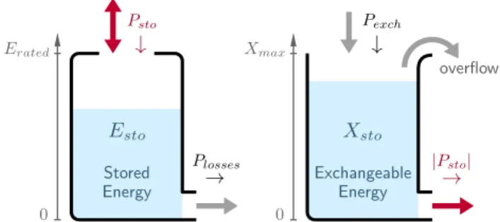
Stored
Energy ExchangeableEnergy
overflow
Figure 2: Graphical representation of the dynamical models for the Energy Storage System and its aging. On the left, the usual stock of stored energy (6). On the right, the aux-iliary stock of “exchangeable energy” (8), which we introduce to enforce aging limi-tation (3).
to highlight how the storage can be seen to act di-rectly as a mitigation of the day-ahead forecast error Pmis.
2.1.2 Energy Storage System
For the purpose of energy management, we need a simple energetic model of the ESS. We use a discrete time model, with ∆t as the time step:
Esto(k + 1) = Esto(k) + (Psto(k) − Plosses)∆t (6)
where Esto is the energy stored in the ESS. Plosses
represents all the energy losses of the storage (in particular: self-discharge and Joule losses) and, in general, is a complex function of Psto and Esto, and
depends on the technology. Since we do not focus on these losses here, we consider a lossless storage: Plosses = 0.
The amount of stored energy Esto is constrained
by the rated energy Er ated:
0 ≤ Esto ≤ Er ated (7)
and we can define the State of Energy: SoE = Esto/Er ated (∈ [0,1]). The dynamical model defined
by (6) is graphically represented on the left side of figure 2.
2.1.3 Exchangeable Energy
As explained in section 1.4, aging limitation can be expressed as an integral constraint (3) on an horizon that is too long. We thus introduce a new auxiliary
state variable to embed constraint (3) in a manageable way. We call it the exchangeable energy stock, with the following dynamical behavior:
Xsto(k+1) = sat(Xsto(k)+(Pexch−|Psto(k)|)∆t) (8)
where Pexch is the mean exchangeable power (4)
and “sat” enables the overflow of this stock beyond a threshold Xmax: sat(x) = x if x 6 Xmax Xmax if x > Xmax (9)
We illustrate this dynamics on the right side of fig-ure 2. A key stage is requiring this stock to be non empty: 0 ≤ Xsto, which translates into a constraint
on the control variable Psto:
|Psto(k)| ≤ Pexch + Xsto(k)/∆t (10)
This constraint is indeed simpler than (3) because it only involves the current value of the state vari-able Xsto. One can show that combining constraint
(10) with the dynamical equation (8) gives a sufficient conditionto respect the original aging limitation (3).
Xsto interpretation: We propose to interpret this
new variable Xsto as a buffer of exchangeable energy.
When the battery is heavily used (|Psto| ≥ Pexch),
this stock decreases. When the battery is less used (|Psto| < Pexch), the stock regenerates. If Xsto
reaches zero, this forces |Psto(k)| ≤ Pexch, which is
a conservative way to respect condition (3). The fi-nite range of Xsto explains that in the long run, the
average of |Psto|is indeed smaller than Pexch.
One downside of this formulation is that it intro-duces the parameter Xmax, the size of the
exchange-able energy stock, which must be chosen. If it is too small, constraint (10) falls back to |Psto(k)| ≤ Pexch
which is stricter than (3). A too big value yields a big stock that the control optimization must manage, so it brings back the problem of a too long optimization horizon. At the end of the article (section 3.4), we extend this qualitative reasoning with numerical re-sults on the effect choosing Xmax. We argue that a
“big enough” size gives enough freedom so that the system performance is eventually the same as with the original constraint (3).
2.1.4 Forecast Error Persistence
Day-ahead forecast error Pmis is a stochastic input for
the ESS control. Also important, it exhibits persis-tence (e.g. positive correlation) along several hours
[10]. We capture both the randomness and the per-sistence using an Autoregressive AR(1) model:
Pmis(k + 1) = ϕPmis(k) + w(k) (11)
where w(k) is a Gaussian white noise.
This AR(1) model has two parameters: the stan-dard deviation σP of Pmis(i.e. the RMS forecast error)
which is linked to the variance of w, and the AR co-efficient ϕ which is the correlation between two suc-cessive hours. Both must be estimated on actual time series [10].
2.2 Control Optimization
Now that we have expressed the system dynamics, we can formulate the control optimization problem. Our control objective is to keep the total output of the wind-storage system (Pдr id = Pprod −Psto) around
the day-ahead commitment P∗
дr id, in a ±Ptol interval.
The control, acting on the storage power Psto, should
minimize on average a penalty at each instant: J =K E1 K−1 X k=0 cost (k) with K → ∞ (12)
where cost (k) is the following penalty function: cost (k) = max(0, |Pdev(k)| − Ptol
)
(13) which penalizes in absolute value each deviation out-side the tolerance band. This penalty with a free tolerance band is inspired by a grid code for wind-storage systems in French islands [10] and can be similarly found in the Hungarian grid code [13, §5.A]. This optimization includes the temporal con-straints introduced with the dynamical equations (6), (8) and (11). The expectation E{} is needed because of the stochastic input w in (11). Therefore, minimizing J is a stochastic dynamic optimization problem [14], which we solve using our open source Stochastic Dy-namic Programming (SDP) packagestodynprog[15].
Note that using SDP is not a requirement for solving the formulation of aging limitation we present here. Another control framework, like the popular Model Predictive Control (MPC, with Koller et. al work [9] as one example) could be used as well.
0.2 0.0 0.2 0.4 0.6 0.8 1.0 1.2 power (pu) P*
grid± 20% Pprod Pgrid
130 132 134 136 138 140 time (days) 0.0 0.2 0.4 0.6 0.8 1.0 SoE
Figure 3: Wind-storage system fulfilling a day-ahead production commitment. Simulation with control C1: optimal ESS control with no ag-ing limitation
3 Aging Control Results
3.1 Input Data
We use the publicly available NREL “Eastern Wind Dataset” [16] as a test case for our aging control method. It provides 3 years of production and day-ahead forecast data3at an hourly timestep (∆t = 1h)
for many wind farms in the US. We choose farm #7277 and normalize the powers by its production ca-pacity (132.3 MW) so that production and forecasts are expressed in per unit (pu). This farm has a mean production of 0.343 pu and RMS forecast error is σP =
0.195 pu. The AR coefficient ϕ, which gives the cor-relation of forecast errors between two successive hours, is estimated at 0.79. This high positive tempo-ral correlation is typically observed with day-ahead forecasts and it adversely impacts the system perfor-mance [10]. On figures 3 and 4, we represent a 10 days extract of this input data (forecast in gray, pro-duction in light blue).
3.2 Test Case
We consider a storage of capacity Er ated = 1 h4.
De-viation tolerance Ptol is set to 0.2 pu (shaded area on
figures 3 and 4). This 20 % tolerance is in line with the
3this dataset is in fact synthetic: production and forecasts are
reconstructed from numerical weather models [17].
4Er ated is expressed in hours when working in per units.
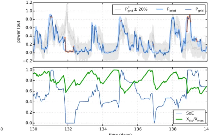
Ac-tual capacity is 1 h×the rated power of the wind farm, which is a typical value in such a context of day-ahead production hedging. 0.2 0.0 0.2 0.4 0.6 0.8 1.0 1.2 power (pu) P*
grid± 20% Pprod Pgrid
130 132 134 136 138 140 time (days) 0.0 0.2 0.4 0.6 0.8 1.0 SoE Xsto/Xmax
Figure 4: Wind-storage system fulfilling a day-ahead production commitment. Simulation with control C3: optimal aging-constrained ESS control
grid code for French islands. For aging limitation, we require a maximum of Nlif e = 3000 equivalent full
cycles over the period Tlif e = 20 years. This gives an
exchangeable power Pexch = 0.034 pu, which is quite
small compared to the RMS forecast error σP. We
choose this (moderately) ambitious aging limitation so that it cannot be reached “by chance”, without an explicit action in the energy management. This way we can show the effectiveness of our aging control. Finally, we set Xmax to 1.71 h (Pexch50 h) but we
ex-plain this choice further, in section 3.4.
We simulate the wind-storage system with differ-ent controls and collect three performance statistics (reported in table 1):
• Aging: the number of equivalent full cycles Ncycle(Tlif e), which we would like to be less
than Nlif e = 3000.
• Ovtol, shorthand for “Over tolerance”: the pro-portion of hourly time steps spent above the tol-erance threshold (|Pdev(k)| > Ptol ).
• Ovtol MAE: Mean Absolute Error above the tol-erance threshold. This is in fact the criterion J minimized by the control, given penalty func-tion (13).
3.3 Simulation Results
For each control strategy, we run the simulation with the entire 3 years dataset and we report the statistics
in table 1. The controls we compare, along their re-spective results, are:
1. C1: optimal control with no aging limitation. This gives the best performance for J (0.013 pu), but aging is twice above the target of 3000 cy-cles/20 yr.
2. C2: we overload C1 with our aging limitation (10) introducing Xsto in the dynamics. Aging
limitation is indeed effective, but the perfor-mance is severely decreased because C1 doesn’t anticipate Xsto evolution. As a consequence,
Xsto value is often zero, or close to, which
im-plies a overly conservative limitation of |Psto| through inequality (10).
3. C3: optimal control with aging limitation (using Xsto): Aging limit is respected, and the
mance (0.014 pu) is not far from the best perfor-mance without aging limitation (C1).
As a baseline reference, C0 gives the performance statistics in the absence of storage. These simula-tions show the effectiveness of our aging control C3 at keeping cycling aging just below the user imposed limit, while still keeping the best possible perfor-mance, like the regular optimal control C1.
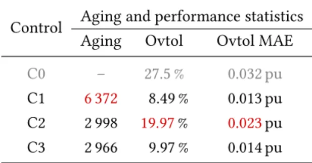
Table 1: Performance comparison Control Aging and performance statistics
Aging Ovtol Ovtol MAE
C0 – 27.5 % 0.032 pu
C1 6 372 8.49 % 0.013 pu
C2 2 998 19.97% 0.023pu
C3 2 966 9.97 % 0.014 pu
To illustrate the qualitative behavior of these two controls, we represent an extract of trajectories with C1 and C3 on figures 3 and 4 respectively. The time periods when |Pdev| > Ptolare highlighted in orange.
One can see that the time spent outside the tolerance band is quite similar between the two. Looking at the SoE (bottom panels), there are more fluctuations for C1 than C3, but the slow (daily) variations are simi-lar. However, we underline that strategy C3 cannot be reduced to a simple linear low-pass filtering of C1. We can observe that with C3, the battery spends more time at rest (Psto = 0 so Pдr id = Pprod and SoE(t) is
constant). All in all, the “thriftier” battery manage-ment C3 is responsible for the reduction in the num-ber of cycles by a factor of two compared with C1. 3.4 Choosing the Aging Control Horizon We have so far left undiscussed the choice of the only tunable parameter of our method: Xmax, the size of
the exchangeable energy stock Xsto. Let us remind
that this stock is used to give freedom to the control to allocate more battery power (i.e. consume cycles) when needed, while still keeping |Psto|below Pexch on average.
For better reasoning, we express this stock size as a time TX using the relation
Xmax = Pexch×TX (14)
Parameter TX is the time it takes to recharge the
entire stock, starting from zero (Xsto stock is indeed
recharged, according to (8), at a rate equal to Pexch).
Thus, from the perspective of aging control, it rep-resents the time horizon on which the ESS control algorithm can borrow exchangeable energy from the future. Therefore, we call TX the aging control
hori-zon.
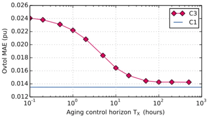
We study its effect by varying its value from zero to 500 hours in our age limiting control C3. We show the resulting performance statistics on figure 5 (red curve). For a too small horizon (TX < 1 h), there is a
major performance loss due to the conservativeness of our aging limitation method. As the horizon is in-creased, the performance loss decreases. Then, for an horizon TX greater than about 100 hours, there is
an optimal plateau as TX → ∞. We thus claim that
our method becomes equivalent to an optimal control satisfying the initial aging constraint (3) that spans over Tlif e (20 years here).
These numerical results support the qualitative reasoning proposed at the end of section 2.1.3. Also, this justifies a posteriori our choice of TX = 50 hours
in our previous simulations: it yields an (almost) op-timal performance while being small enough to en-sure the fastest convergence of the SDP optimization algorithm5.
Finally, we can observe on figure 5 a performance gap of about 0.001 pu between C3 and C1 (control
5more precisely, we use a “policy iteration” algorithm [14, 15].
It includes iterations along time in each “policy evaluation” step, and the number of those iterations is dictated by the time constants of all stocks, e.g. TX.
10-1 100 101 102 103
Aging control horizon TX (hours)
0.012 0.014 0.016 0.018 0.020 0.022 0.024 0.026
Ovtol MAE (pu)
C3 C1
Figure 5: Effect of the aging control horizon on the performance of the optimal aging-constrained control C3. A too small TX
(under ∼100 h) yields a too conservative aging limitation which decreases the per-formance. As a baseline, control C1 with no aging limitation shows the perfor-mance difference due to the aging limita-tion constraint.
without aging limitation, blue line). We claim that this is the price of the aging constraint (a constrained minimum is always worse or equal than a constraint-free one). A further study could be to vary the aging limit (3000 cycles on 20 years in this article) to gen-erate a trade-off curve between the performance and the limit. This would outline a Pareto front between these two conflicting objectives (minimizing output deviations and cycling aging).
4 Conclusion
We introduced a formulation of cycling aging (based on exchanged energy counting) with two advan-tages: it fits naturally in the ESS control optimiza-tion and it enables the control designer to directly set a maximum number of battery cycles over the project lifetime. We illustrated the effectiveness of our scheme with a simulation on an open dataset. On this example, cycling is reduced by 50 % with a less than 10 % decrease in performance.
Further studies could include looking at the trade-off between the limitation of storage aging and the performance. Also, we plan to adapt our formalism to other aging models, in particular weighted charge counting [3,4], and more importantly calendar aging. Calendar aging can be included in control optimiza-tion when it depends on operaoptimiza-tional condioptimiza-tions like
SoE (particularly true for super capacitors [1]).
Acknowledgment
We are grateful to NREL for providing the Eastern Wind dataset [16,17] which is very useful as an open benchmark for simulations of wind-storage systems.
References
[1] T. Kovaltchouk, B. Multon, H. Ben Ahmed, J. Aubry, and P. Venet, “Enhanced Aging Model for Supercapacitors taking into account Power Cycling: Application to the Sizing of an Energy Storage System in a Direct Wave Energy Con-verter,” in 9th Ecological Vehicles and Renewable Energies (EVER) 2014 conference, Monte Carlo, Monaco, Mar. 2014.
[2] J. Aubry, P. Bydlowski, B. Multon, H. Ben Ahmed, and B. Borgarino, “Energy Storage Sys-tem Sizing for Smoothing Power Generation of Direct Wave Energy Converters,” in 3rd Interna-tional Conference on Ocean Energy, 2010. [3] H. Bindner, T. Cronin, P. Lundsager, J. F.
Man-well, U. Abdulwahid, and I. Baring-Gould, “Life-time Modelling of Lead Acid Batteries ,” Risø National Laboratory, Tech. Rep., Apr. 2005. [4] D. U. Sauer and H. Wenzl, “Comparison of
different approaches for lifetime prediction of electrochemical systems—Using lead-acid bat-teries as example,” Journal of Power Sources, vol. 176, no. 2, pp. 534–546, 2008.
[5] L. Serrao, S. Onori, G. Rizzoni, and Y. Guezen-nec, “A novel model-based algorithm for bat-tery prognosis,” in Proceedings of the Seventh IFAC Symposium on Fault Detection, Supervision and Safety of Technical Processes (SAFEPROCESS 09), 2009.
[6] P. Haessig, “Dimensionnement & gestion d’un stockage d’´energie pour l’att´enuation des incer-titudes de production ´eolienne,” Ph.D. disserta-tion, ENS Cachan, Jul. 2014.
[7] L. Serrao, S. Onori, A. Sciarretta, Y. Guezen-nec, and G. Rizzoni, “Optimal energy man-agement of hybrid electric vehicles including
battery aging,” in American Control Conference (ACC), 2011, June 2011, pp. 2125–2130.
[8] H. Borhan, M. A. Rotea, and D. Viassolo, “Optimization-based power management of a wind farm with battery storage,” Wind Energy, vol. 16, no. 8, pp. 1197–1211, Nov. 2013.
[9] M. Koller, T. Borsche, A. Ulbig, and G. Ander-sson, “Defining a degradation cost function for optimal control of a battery energy storage sys-tem,” in IEEE PowerTech 2013 Conference, Greno-ble, France, Jun. 2013.
[10] P. Haessig, B. Multon, H. Ben Ahmed, S. Las-caud, and P. Bondon, “Energy storage sizing for wind power: impact of the autocorrelation of day-ahead forecast errors ,” Wind Energy, vol. 18, no. 1, pp. 43–57, Jan. 2015, published on-line Oct 2013.
[11] P. Haessig, B. Multon, H. Ben Ahmed, S. Las-caud, and L. Jamy, “Aging-aware NaS battery model in a stochastic wind-storage simulation framework ,” in IEEE PowerTech 2013 Conference, Grenoble, France, Jun. 2013.
[12] G. Giebel, R. Brownsword, G. N. Kariniotakis, M. Denhard, and C. Draxl, “The state-of-the-art in short-term prediction of wind power: A literature overview,” ANEMOS.plus, Tech. Rep., 2011.
[13] B. Hartmann and A. D´an, “Cooperation of a Grid-Connected Wind Farm and an Energy Storage Unit — Demonstration of a Simulation Tool,” IEEE Trans. Sustain. Energy, vol. 3, no. 1, pp. 49–56, Jan. 2012.
[14] D. P. Bertsekas, Dynamic Programming and Op-timal Control, 3rd ed. Athena Scientific, 2005. [15] P. Haessig, T. Kovaltchouk, B. Multon, H. Ben
Ahmed, and S. Lascaud, “Computing an Opti-mal Control Policy for an Energy Storage,” in 6th European Conference on Python in Science (EuroSciPy 2013), Brussels, Belgium, Aug. 2013, pp. 51–58.
[16] National Renewable Energy Laboratory, “East-ern Wind Integration and Transmission Study,” Tech. Rep. NREL/SR-5500-47078, Feb. 2011.
[17] AWS Truewind, “Development of Eastern Re-gional Wind Resource and Wind Plant Output Datasets: March 3, 2008 - March 31, 2010,” Tech. Rep. NREL/SR-550-46764, Dec. 2009.