Boundary Extraction in Natural Images Using Ultrametric Contour Maps
Pablo Arbel´aez
CEREMADE, UMR CNRS 7534 Universit´e Paris Dauphine,
Place du mar´echal de Lattre de Tassigny, 75775 Paris cedex 16, France
Abstract
This paper presents a low-level system for boundary ex-traction and segmentation of natural images and the eval-uation of its performance. We study the problem in the framework of hierarchical classification, where the geomet-ric structure of an image can be represented by an ultra-metric contour map, the soft boundary image associated to a family of nested segmentations. We define generic ultra-metric distances by integrating local contour cues along the regions boundaries and combining this information with gion attributes. Then, we evaluate quantitatively our re-sults with respect to ground-truth segmentation data, prov-ing that our system outperforms significantly two widely used hierarchical segmentation techniques, as well as the state of the art in local edge detection.
1. Introduction
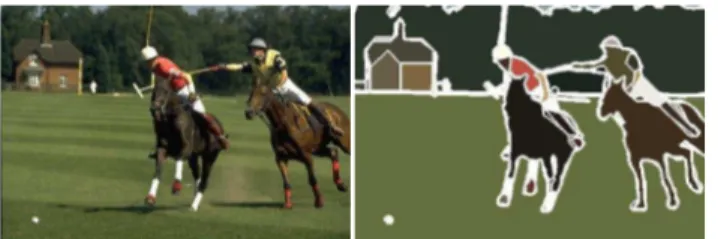
Hierarchical organization is one of the main characteris-tics of human segmentation. A human subject segments a natural image by identifying physical objects and marking their boundaries up to a certain level of detail. If we suppose that different subjects segmenting a single image perceive the same objects then, up to variations in the exact localiza-tion of boundaries, the interseclocaliza-tion of their segments deter-mines the finest level of detail considered. Figure1presents an example, with a natural image and six human segmenta-tions from [9]. The segmentations are superimposed and the segments are represented by their mean color.
Segmentation can be thought as a process of grouping vi-sual information, where the details are grouped into objects, objects into classes of objects, etc. Thus, starting from the composite segmentation, the perceptual organization of the image can be represented by a tree of regions, ordered by inclusion. The root of the tree is the entire scene, the leaves are the finest details and each region represents an object at a certain scale of observation.
In this paper, we study the segmentation problem in the framework of data classification, where the notions of tree
Figure 1. Natural image and composite human segmentation.
of regions and scale are formalized by the structure of in-dexed hierarchy or, equivalently, by the definition of an ul-trametric distance on the image domain. We present a for-mulation of the problem in terms of contours that allows to represent an indexed hierarchy of regions as a soft boundary image called ultrametric contour map.
Since the early days of computer vision, the hierarchical structure of visual perception has motivated clustering tech-niques to segmentation [13], where connected regions of the image domain are classified according to an inter-region dissimilarity measure. We consider the traditional bottom-up approach, also called agglomerative clustering, where the regions of an initial partition are iteratively merged, and we characterize those dissimilarities that are equivalent to ultrametric distances.
The key point of hierarchical classification is the defini-tion of a specific distance for a particular applicadefini-tion. We design ultrametrics for contour extraction by integrating and combining local edge evidence along the regions bound-aries and complementing this information with intra-region attributes.
In order to design a generic segmentation system, all its degrees of freedom are expressed as parameters, whose tuning we interpret as the introduction of prior knowledge about the objects geometry. This information is provided by a database of human segmentations of natural images [9]. We optimize our system with respect to this ground-truth data and evaluate quantitatively our results using the Precision-Recall framework [8]. With this methodology, we prove that our system outperforms significantly two
ods of reference in segmentation by clustering, the varia-tional approach of [7] and the hierarchical watersheds [12]. Furthermore, we show that the performance of our method is superior to state of the art local edge detectors [8], while providing a set of closed curves for any threshold.
2. Definitions
2.1. Hierarchical Segmentation
Let Ω ⊂ R2 be the domain of definition of an image,
P0an initial partition of Ω and λ ∈ R a scale parameter. A
hierarchical segmentation operator (HSO) is an application
that assigns a partition Pλto the couple (P0, λ), such that
the following properties are satisfied:
Pλ= P0, ∀λ ≤ 0 (1)
∃ λ1∈ R+ : Pλ= {Ω}, ∀λ ≥ λ1 (2)
λ ≤ λ0⇒ P
λv Pλ0 (3)
Relations (1) and (2) determine the effective range of scales of the operator and indicate that the analysis can be restricted to the interval [0, λ1]. The symbol v denotes the
partial order of partitions : P v P0 ⇔ ∀ a ∈ P, ∃ b ∈
P0 : a ⊆ b. Thus, relation (3) sets that partitions at
dif-ferent scales are nested, imposing a hierarchical structure to the family H = {R ⊂ Ω | ∃λ : R ∈ Pλ}.
By considering the scale where a region appears in H, one can then define a stratification index, the real valued application f given by :
f (R) = inf{λ ∈ [0, λ1] | R ∈ Pλ}, ∀ R ∈ H (4)
The couple (H, f ) is called an indexed hierarchy of sub-sets of Ω. It can be represented by a dendrogram, where the height of a region R is given by f (R). The construction of (H, f ) is equivalent to the definition of a distance between two elements x, y of P0:
Υ(x, y) = inf{f (R) | x ∈ R ∧ y ∈ R ∧ R ∈ H}. (5) The application Υ belongs to a special type of distances called ultrametrics that, in addition to the usual triangle in-equality, satisfy the stronger relation :
Υ(x, y) ≤ max{Υ(x, z), Υ(z, y))}. (6)
2.2. Ultrametric Contour Maps
We now follow [10] for the definition of a segmentation in terms of contours in a continuous domain.
A segmentation K of an image u as a finite set of rec-tifiable Jordan curves, called the contours of K. The
re-gions of K, noted (Ri)i are the connected components of
Ω \ K. Furthermore, we suppose that the contours meet
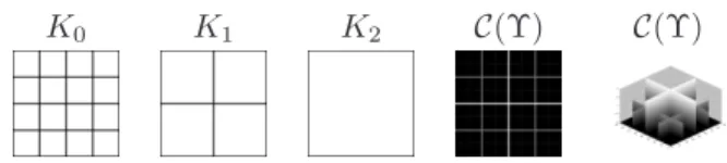
K0 K1 K2 C(Υ) C(Υ)
Figure 2. From left to right : Family of segmentations defined by a HSO, UCM and 3D view of UCM.
each other and ∂Ω only at their tips, that each contour sepa-rates two different regions and that each tip is common to at least three contours. The contour separating regions Riand
Rjis noted ∂ij.
Hence, a segmentation can be equivalently expressed by its contours K or by the partition P = {Ri}iof Ω.
Rewriting properties (1) to (3) in terms of contours of the segmentations leads to the following characterization of a HSO :
Kλ= K0, ∀λ ≤ 0 (7)
Kλ= ∂Ω, ∀λ ≥ λ1 (8)
λ ≤ λ0⇒ Kλ⊇ Kλ0 (9)
Relation (7) determines the set of initial contours K0and (8)
indicates that all inner contours vanish at finite scale. The hierarchical structure imposed by (9), called the principle of
strong causality in [10], establishes that the localization of contours is preserved through the scales.
We can now define the model of contours that will be considered.
Let Υ be the ultrametric distance defined by a HSO. The ultrametric contour map (UCM) associated to Υ is the application C(Υ) : K0→ [0, λ1] given by:
C(Υ)(∂) = inf{λ ∈ [0, λ1] | ∂ * Kλ}, ∀ ∂ ∈ K0. (10)
The number C(Υ)(∂) is called the saliency of contour ∂. Note the duality with the regions, the saliency of ∂ being its
scale of disappearance from the hierarchy of contours.
The ultrametric contour map is a representation of a HSO in a single real-valued image. Figure2presents a simple ex-ample of UCM. By definition, thresholding this soft bound-ary image at scale λ provides a set of closed curves, the segmentation Kλ.
Nevertheless, note that if the initial partition P0is fixed,
all the UCM weight the elements of the same set K0.
Hence, the utility of such a representation is determined by the distance Υ, whose value defines the saliency of each contour. Our objective will be to design ultrametrics such that the UCM model the boundaries of physical objects in natural images.
3. Ultramteric Dissimilarities
3.1. Region Merging
The ascending construction of a family of nested par-titions is one of the earliest approaches to segmentation [10,4]. These region merging techniques are principally de-termined by two elements : the choice of an initial partition
P0and the definition of a dissimilarity measure δ between
couples of adjacent regions.
Such a merging process can be implemented efficiently by using a region adjacency graph (RAG) [14,6]. A RAG is an undirected graph where the nodes represent connected regions of the image domain. The links encode the adja-cency relation and are weighted by the dissimilarity. The RAG is initialized with P0 and the family of partitions is
obtained by removing the links for increasing values of the dissimilarity and merging the corresponding nodes.
In the huge literature on the subject, the initial partition is typically an over-segmentation in very homogeneous re-gions, e.g. the partition in pixels, in connected components or the result of a pre-processing. The dissimilarity measure is defined from the image data. One can for instance con-sider a piecewise regular approximation of the initial image and measure the dissimilarity by comparing the approxima-tions of adjacent regions.
3.2. Defining the Distance
Starting from a family of nested partitions constructed by a region merging process, one can always define an ul-trametric distance by considering as stratification index an increasing function of the merging order. However, in order to define a meaningful notion of scale, the distance between any two points in adjacent regions should coincide with the inter-region dissimilarity δ:
Υ(x, y) = δ(Ri, Rj), ∀x ∈ Ri, ∀y ∈ Rj. (11)
This property is satisfied by setting the value of the dissim-ilarity at the creation of a region as its stratification index. However, for an arbitrary dissimilarity, this choice can lead to the existence of two regions (R, R0) ∈ H2 such that
R ⊂ R0 but f (R) > f (R0). In terms of contours, this
situation implies the violation of strong causality (9). Hence, we call δ an ultrametric dissimilarity if the cou-ple (H, f ) is an indexed hierarchy, where f is defined by :
f (Ri∪ Rj) = δ(Ri, Rj), (12)
for all couples of connected regions (Ri, Rj) ∈ H2.
One can then prove that a dissimilarity δ is ultrametric if and only if
δ(Ri, Rj) ≤ δ(Ri∪ Rj, R), (13)
where (Ri, Rj) is a couple of regions that minimizes δ and
R is a region connected to Ri ∪ Rj and belonging to the
partition obtained after the merging of (Ri, Rj).
In order to stress the fact that ultrametric dissimilarities define distances in P0, they are noted Υ in the sequel.
Working with ultrametric dissimilarities, as those de-fined in the next section, is important for our application because it guarantees that the saliency of each contour in the UCM is exactly the value of the dissimilarity between the two regions it separates.
4. Ultrametrics for Boundary Extraction
We now turn to the problem of defining specific dis-tances for the extraction of boundaries in natural images. For this purpose, our strategy consists in measuring local contour evidence along the common boundary of regions, and then complementing this information with internal re-gion attributes. In order to design a generic low-level sys-tem, all the degrees of freedom are expressed as parameters.
4.1. A Contrast Ultrametric
We first define a distance that uses the color informa-tion of the initial image for measuring the contrast between regions. For this purpose, we represent a color image u with the L∗ab standard [15], an approximation of the
per-ceptually uniform color space. The distance between two colors in L∗ab is usually measured by the Pythagorean
for-mula; however, in order to tolerate variations in the relative weight of lightness and chrominance, we propose the fol-lowing distance d∗ between two colors k = (l, a, b) and
k0= (l0, a0, b0) :
d∗(k, k0) =p(l − l0)2+ ξ(a − a0)2+ ξ(b − b0)2. (14)
With this color representation, monochromatic images cor-respond to the particular case ξ = 0 and the usual L∗ab
space to ξ = 1.
In order to determine the presence of a boundary, we de-fine a local contrast measure at a point x ∈ Ω by the for-mula:
τ (u, x) = sup{d∗(u(y), u(y0)) | ∀ y, y0∈ B
r(x)}, (15)
where Br(x) denotes a Euclidian ball of radius r centered
at x.
Our first distance is given by the mean local contrast along the common boundary of regions:
Υc(Ri, Rj) = Σc(∂ij)
L(∂ij), (16)
where L(∂) denotes the length of the contour ∂ and Σc(∂)
is given by :
Σc(∂) =
Z
∂
The interest of distance Υcis that, being defined on the
initial image u, the set K0of initial contours coincides with
the discontinuities of u. Thus, the associated UCM preserve the localization of the original boundaries.
4.2. A Boundary Ultrametric
The distance Υc expresses a notion of homogeneity of
objects based only on color uniformity. In order to consider a larger class of contour cues, we use as input to our system the result of a local edge detector, noted g. In the exam-ples presented, we used the detector of [8], that measures and combines optimally local cues as brightness, color and texture.
As in the previous paragraph, we consider a mean
bound-ary gradient distance:
Υg(Ri, Rj) = Σg(∂ij) L(∂ij) , (18) where Σg(∂) = Z ∂ g(x(s))ds. (19)
Then, the weighted sum of mean boundary gradient and mean contrast of the initial image defines our final boundary
ultrametric:
ΥB(Ri, Rj) = Υc(Ri, Rj) + α1· Υg(Ri, Rj), (20)
where α1≥ 0.
4.3. Considering Region Attributes
In order to take into account the internal information of regions in the distance, we measure an attribute on each re-gion, a function A : P(Ω) → R+, increasing with respect
to the inclusion order : R ⊂ R0⇔ A(R) < A(R0).
Thus, starting from (20), we define the following generic notion of scale for boundary extraction:
ΥS(Ri, Rj) = ΥB(Ri, Rj) · min{A(Ri), A(Rj)}α2,
(21) where α2≥ 0. Note that, since the term Υcnever vanishes,
the UCM associated to ΥBand ΥSpreserve the localization
of the contours of the initial image.
In the experiments presented in this paper, we used as attribute a linear combination of area and total quadratic er-ror: A(R) = Z R dx + α3· Z R d∗(u(x), M (R))2dx (22) where α3 ≥ 0 and M (R) denotes the mean color of u on
region R.
We considered two methods for introducing the internal information in the distance. The first one is to use directly the UCM associated to ΥS. The second one consists in
pruning the tree of ΥBfor increasing values of ΥS.
4.4. Initial Set of Contours
We have discussed so far the definition of distances meaningful for our application. We now address the issue of choosing an appropriated set of initial contours K0. For
this purpose, in absence of prior knowledge about the image content, we do the methodological choice of preserving the inclusion relation between the discontinuities of the origi-nal image and K0. This amounts to supposing that a
con-nected region where the image is constant cannot belong to two different objects. This property is satisfied by the pre-segmentation method we now describe.
The objective of pre-segmentation is to decompose the image in local entities, more coherent and less numerous than pixels, while preserving its geometric structure. For this purpose, we exploit the fact that ultrametric dissimi-larities define pseudo-metrics on the image domain. Pre-cisely, we produce an over-segmentation by considering the extrema of the L∗channel in the original image and
associ-ating each point of Ω to the closest extremum in the sense of ΥS. This construction defines a Voronoi tessellation of
the domain; a pre-segmented image is then obtained by as-signing a constant color to each region.
Thus, the method produces a reconstruction of the orig-inal image from the information of its lightness extrema, that preserves the localization of the original contours. De-pending on the image, the pre-segmentation can be iterated a few times without affecting the main geometric structures. Its degrees of freedom are treated as additional parameters of our system.
4.5. Examples
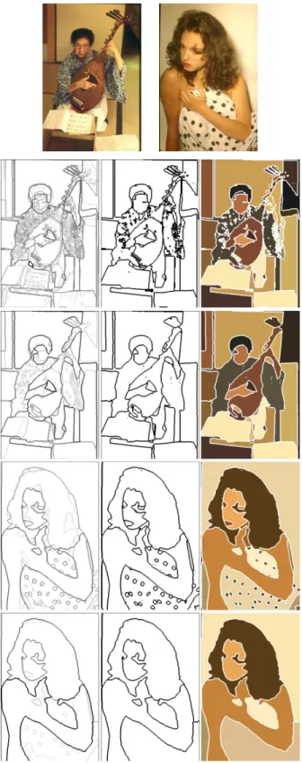
Figure3illustrates the influence on the output of our sys-tem of the different types of information considered in the proposed notion of scale. Lines 2 to 5 present, from left to right, the UCM, the segmentation given by the optimal scale of the UCM with respect to human-marked boundaries (see Section 5.1) and the corresponding reconstruction, where the segments are represented by their mean color. The dis-tance Υcof Line 2 measures only the contrast of the original
image. As a consequence, textured regions as the dress are a source of noise in the UCM. The saliency of these regions is reduced in the boundary ultrametric ΥB(Line 3) by
choos-ing a local detector that measures texture homogeneity. The second example shows the utility of considering internal re-gion attributes (Line 5) as a complement to plain boundary information (Line 4). On the one hand, it eliminates small imperfections of the image. On the other hand, it allows to control the saliency of structures like the dark dots, whose size triggers the response of the local detector, but whose importance may depend on the application.
Figure 3. Examples. Line 1: original images. Lines 2 to 5. From left to right : UCM, segmentation and reconstruction. From top to bottom: C(Υc), C(ΥB), C(ΥB) and C(ΥS).
5. Evaluation of Results
5.1. Methodology
Our system combines several types of low-level image information into a single notion of scale, the saliency of boundaries in the UCM. We interpret the tuning of its pa-rameters as the introduction of prior information about the geometric structure of the image. In order to measure quan-titatively the pertinence of our approach and compare it to other methods, the system was optimized using the Berkeley
Segmentation Dataset and Benchmark (BSDB) [1]. In this study, the ground-truth data is provided by a large database of natural images, manually segmented by human subjects [9]. A methodology for evaluating the performance of boundary detection techniques with this database was de-veloped in [8]. It is based in the comparison of machine-detected boundaries with respect to human-marked bound-aries using the Precision-Recall framework, a standard in-formation retrieval technique. Precisely, two quality mea-sures are considered, Precision (P), defined as the fraction of detections that are true boundaries and Recall (R), given by the fraction of true boundaries that are detected. Thus, Precision quantifies the amount of noise in the output of the detector, while Recall quantifies the amount of ground-truth detected. Measuring these descriptors over a set of images for different thresholds of the detector provides a parametric
Precision-Recall curve. The two quantities are then
com-bined in a single quality measure, the F-measure, defined as their harmonic mean:
F (P, R) = 2P R
P + R. (23)
Finally, the maximal F-measure on the curve is used as a summary statistic for the quality of the detector on the set of images.
The current public version of the BSDB is divided in two independent sets of images. A training set of 200 images and a test set of 100 images. In order to ensure the in-tegrity of the evaluation, only the images and segmentations from the training set can be accessed during the optimiza-tion phase. The algorithm is then benchmarked by using the optimal training parameters “blindly” on the test set.
5.2. Tested Methods
The BSDB is a standard experimental protocol that al-lows the comparison of different boundary detection tech-niques by quantifying their performance with respect to hu-man vision. Furthermore, since the quality of a detector is judged exclusively on the accuracy of the contours it pro-duces, the methodology permits a direct comparison be-tween local edge detection and region-based segmentation approaches. Although its use in the segmentation commu-nity is nowadays widespread, only the former have been
evaluated to our knowledge (see [8]). Estrada and Jep-son [3] compared recently four region-based segmentation methods within the same framework. However, it should be noted that their study uses a different experimental setup and considers only gray-level images.
Our evaluation work was divided in two parts. First, op-timizing and benchmarking our system in order to compare it to already benchmarked local edge detectors. Second, we benchmarked two methods of reference in hierarchical seg-mentation and compared their results with ours. The opti-mization phase was carried out using a steepest ascent in the F-measure. In all the experiments, we used the imple-mentations made available by the authors. We now describe briefly the tested algorithms.
5.2.1 Local Edge Detectors
The state of the art in local boundary detection techniques is the system proposed in [8, 1]. The gradient paradigm implemented by Martin et al. relies on the measure, at each pixel, of local discontinuities in feature channels like bright-ness, color and texture, over a range of scales and orienta-tions. Local cues are combined and optimized with respect to the BSDB. Then, using the Precision-Recall framework, the authors show that their detector, noted in the sequel MFM, outperforms all other local edge detection methods.
We used the MFM as a reference of local detection meth-ods and as an input to our system. Additionally, the Canny detector, based on an estimation of the gradient magnitude of brightness and non-maxima suppression, provided the baseline in classical local approaches. For both methods, we used the codes distributed with the BSDB with their de-fault optimized parameters.
5.2.2 Hierarchical Watersheds
As a reference of a hierarchical segmentation operator based only the information of a gradient image, we used the work of Najman and Schmitt [12,2], who study the ul-trametric contour map associated to the watershed segmen-tation. To our knowledge, these authors were the first to consider explicitly the soft contour image associated to a family of nested segmentations for boundary detection pur-poses.
This method is based on the construction of the water-shed by a flooding process. A gradient image, seen as a topographic surface, is pierced at its minima and progres-sively immersed in water. The water fills the catchment basins of the minima and forms lakes. When two lakes meet, the level of the water (the height of the saddle point) determines the saliency of the corresponding watershed arc. Thus, the notion of scale of this technique is an estimation of the contrast between two regions by the minimal value of the gradient on their common boundary.
A natural choice for the topographic surface seems to be the MFM detector. However, following the Canny ap-proach, the MFM considers only the maxima in the gradient direction. As a consequence, the final output of the MFM has often a single regional minimum and, in the presence of a unique lake, the watershed is empty. Thus, we used as topographic surface the MFM detector before non-maxima suppression. This choice has the interest of providing a wa-tershed for color images, with regular contours and robust to noise and texture.
5.2.3 Variational Approach
The formulation of the segmentation problem in the varia-tional framework is one of the most popular approaches of the recent years. In order to compare our results to a HSO based exclusively on the information of the original image, we used the work of Koepfler et al. [7,10,5], who propose a multi-scale approach for the minimization of the piecewise constant version of the Mumford and Shah functional [11]. This study considers a region merging process, where the criterion to merge two regions is to decrease the value of the global energy:
E(K) =
Z
Ω\K
km − uk2dx + λL(K) , (24)
where m denotes the piecewise constant approximation of the initial image u by the mean color in each region. Hence, with this approach, the objects in the image are modelled as regions of homogenous color with short boundaries. The dissimilarity governing this merging process is given by:
δM S(Ri, Rj) = |Ri| · |Rj|
|Ri| + |Rj|·
kM (Ri) − M (Rj)k2
L(∂ij) , (25)
where |R| denotes the area of region R. Thus, δM S is the
squared absolute difference of the mean color in the re-gions, combined with two other factors. The first one is proportional to the harmonic mean of the areas and elimi-nates small regions from the segmentation. The second one is the inverse of the boundary length. This information con-trols the regularity of the result, since, if the other factors of
δM Sare identical, the couple of regions with longest
com-mon boundary is merged first. However, note that the dis-similarity δM Sis not ultrametric. In order to restore strong
causality, we constructed the UCM of this method by super-imposing the results for increasing values of the parameter
λ in (24).
In order to make the comparison with our system fair, we used the L∗ab space with the weight ξ in (14) tuned for this
algorithm. Additionally, we optimized as initial image the result of the pre-segmentation method described in Section
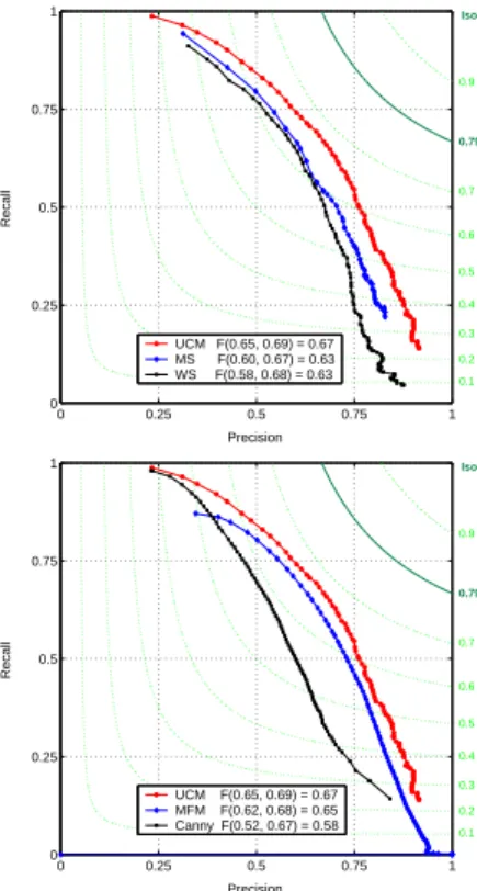
0 0.25 0.5 0.75 1 0 0.25 0.5 0.75 1 Precision Recall UCM F(0.65, 0.69) = 0.67 MS F(0.60, 0.67) = 0.63 WS F(0.58, 0.68) = 0.63 0.9 0.79 0.7 0.6 0.5 0.4 0.3 0.2 0.1 IsoF 0 0.25 0.5 0.75 1 0 0.25 0.5 0.75 1 Precision Recall UCM F(0.65, 0.69) = 0.67 MFM F(0.62, 0.68) = 0.65 Canny F(0.52, 0.67) = 0.58 0.9 0.79 0.7 0.6 0.5 0.4 0.3 0.2 0.1 IsoF
Figure 4. Evaluation results. Up: our UCM compared to other clustering techniques. Down: our UCM compared to local edge detectors
5.3. Results
The results of the evaluation on the test set are presented in Figure4. The dotted (green) lines represent the isolevel lines of the function F (P, R) defined by (23), with values on the right. They can be used to situate the Precision-Recall curves, since the quality of a detector is judged by considering the image of its curve by F . Thus, the point with maximal F-measure can be interpreted as the high-est point of the curve on the surface z = F (P, R), the objective being the point F (1, 1) = 1. The isolevel line
F (P, R) = 0.79 corresponds to the human consistency on
this set of images, obtained by comparing the human seg-mentations among them. This line represents the reference with respect to which the performance of machines for the task of boundary extraction is measured.
It can be observed that the Precision-Recall curve of our system (UCM) dominates significantly all the others. Hence, for a given amount of noise tolerated (fixed Pre-cision), our UCM detect a greater fraction of true bound-aries (higher Recall). Conversely, for a required amount of ground-truth detected (fixed Recall), our results are those with less noise (higher Precision).
The top panel shows the curves corresponding to the three HSOs benchmarked. Although the scores of the varia-tional approach (MS) and the hierarchical watersheds (WS)
are very close, the curve of the former dominates that of the latter. However, both methods are significantly outper-formed by our system. The hierarchical watershed exploits the information of a gradient image, while the variational approach considers only the original image. The superior-ity of our UCM comes from the generic combination of both types of information.
The bottom panel compares our UCM with two local detectors already benchmarked on the BSDB: the classi-cal Canny method and the top-ranked MFM. As before, our curve clearly dominates the two others. Nevertheless, more than the score, the main improvement of our system with respect to local detectors is to provide for any scale a set of closed curves, the contours of a segmentation.
Figures5and6present some qualitative results, all ob-tained with the optimal training parameters of each algo-rithm. In order to make the results completely automatic, the segmentation shown corresponds to the global optimal scale on the train set. Note that although our system was optimized using only boundary information, the segments obtained coincide often with physical objects or their con-nected parts.
Figure6compares the four tested methods on an exam-ple. It can be observed that our model of boundaries pro-vides the best trade-off between accuracy and noise, allow-ing the extraction of the main geometric structures in the images. The improvement of our UCM with respect to the variational approach is in part due to the explicit treatment of texture of the local detector. The watersheds present the more regular contours among the tested methods and dis-play a typical mosaic effect, where the lakes of the topo-graphic surface are discernable in the contour map. Finally, the MFM results are shown to illustrate the essential differ-ence in initial orientation between local and region-based approaches. The level of representation is the point for the former and the region for the latter. As a consequence, local detectors require in many applications a contour completion post-processing in order to integrate their information into closed curves.
6. Conclusions
This paper presented the design and evaluation of a novel boundary extraction system. Its main characteristic is to rely on the formulation of the problem in the framework of hierarchical classification, which allows to address region-based segmentation and edge detection as a single task.
We defined generic ultrametric distances for this spe-cific application and showed the interest of the approach followed by evaluating our results with a standard method-ology. Additionally, we evaluated with the same protocol two methods of reference in hierarchical segmentation.
Although the introduction of semantic information seems necessary in order to fill the still large gap with
hu-Figure 5. Results of our system. From left to right : Original im-ages, automatic segmentation and UCM.
man performance for this task, we are confident that higher-level approaches can benefit from our low-higher-level representa-tion of the image boundaries.
References
[1] The Berkeley Segmentation Dataset and Benchmark. www.cs.berkeley.edu/projects/vision/grouping/segbench/.5,
6
[2] M. Couprie. Library of operators in image processing PINK. http://www.esiee.fr/ coupriem.6
[3] F. Estrada and A. Jepson. Quantitative evaluation of a novel image segmentation algorithm. In Proc. CVPR’05, pages II: 1132–1139, 2005.6
[4] D. Forsyth and J. Ponce. Computer Vision: A Modern Ap-proach. Prentice Hall, 2003.3
[5] J. Froment and L. Moisan. Image process-ing software megawave. http://www.cmla.ens-cachan.fr/Cmla/Megawave/.6
Figure 6. Comparison of the four tested methods (see text). [6] L. Garrido, P. Salembier, and D. Garcia. Extensive operators
in partition lattices for image sequence analysis. IEEE Trans. on Signal Processing, 66(2):157–180, Apr. 1998.3
[7] G. Koepfler, C. Lopez, and J. Morel. A multiscale algorithm for image segmentation by variational method. SIAM Jour-nal on Numerical AJour-nalysis, 31(1):282–299, 1994.2,6
[8] D. Martin, C. Fowlkes, and J. Malik. Learning to detect nat-ural image boundaries using local brightness, color and tex-ture cues. IEEE Trans. on PAMI, 26(5):530–549, 2004.1,2,
4,5,6
[9] D. Martin, C. Fowlkes, D. Tal, and J. Malik. A database of human segmented natural images and its application. In Proc. ICCV’01, volume II, pages 416–423, 2001.1,5
[10] J. Morel and S. Solimini. Variational Methods in Image Seg-mentation. Birkhauser, 1995.2,3,6
[11] D. Mumford and J. Shah. Optimal approximations by piece-wise smooth functions and variational problems. CPAM, 42(5):577–684, 1989.6
[12] L. Najman and M. Schmitt. Geodesic saliency of water-shed contours and hierarchical segmentation. IEEE Trans. on PAMI, 18(12):1163–1173, 1996. 2,6
[13] R. Ohlander, K. Price, and R. Reddy. Picture segmentation by a recursive region splitting method. Computer Graphics Image Processing, 8:313–333, 1978.1
[14] T. Vlachos and A. Constantinides. Graph-theoretical ap-proach to colour picture segmentation and contour classifi-cation. In IEE Proc. Vision, Image and Sig. Proc., volume 140, pages 36–45, Feb. 1993.3
[15] G. Wyszecki and W. Stiles. Color Science: Concepts and Methods, Quantitative Data and Formulas. J. Wiley and Sons, 1982.3
![Figure 6. Comparison of the four tested methods (see text). [6] L. Garrido, P. Salembier, and D](https://thumb-eu.123doks.com/thumbv2/123doknet/2487724.50761/8.918.79.428.107.664/figure-comparison-tested-methods-text-l-garrido-salembier.webp)