Genomic selection of dairy cows

(1)

HAL Id: pastel-00954581

https://pastel.archives-ouvertes.fr/pastel-00954581

Submitted on 3 Mar 2014

HAL is a multi-disciplinary open access

archive for the deposit and dissemination of sci-entific research documents, whether they are pub-lished or not. The documents may come from teaching and research institutions in France or abroad, or from public or private research centers.

L’archive ouverte pluridisciplinaire HAL, est destinée au dépôt et à la diffusion de documents scientifiques de niveau recherche, publiés ou non, émanant des établissements d’enseignement et de recherche français ou étrangers, des laboratoires publics ou privés.

To cite this version:

Romain Dassonneville. Genomic selection of dairy cows. Animal genetics. AgroParisTech, 2012. English. �pastel-00954581�

(2)

présentée et soutenue publiquement par

Romain DASSONNEVILLE

le 28 septembre 2012

Genomic selection of dairy cows

Sélection génomique des vaches laitières

Doctorat ParisTech

T H È S E

pour obtenir le grade de docteur délivré par

L’Institut des Sciences et Industries

du Vivant et de l’Environnement

(AgroParisTech)

Spécialité : Génétique animale

Directeur de thèse : Vincent DUCROCQ Co-encadrement de la thèse : Didier BOICHARD

Représentant entreprise, Institut de l’Élevage : Sophie MATTALIA

Jury

M.Georg THALLER, Professeur, CAU - Kiel - Allemagne Rapporteur

M. Johan SÖLKNER, Professeur, BOKU – Vienne - Autriche Rapporteur

M. Sander DE ROOS, Docteur, responsable schéma de sélection CRV – Arnhem – Pays-Bas Examinateur

M. Pierre-Louis GASTINEL, chef du département génétique, Institut de l’Élevage, Paris Examinateur

M. Thomas HEAMS, Docteur, Maître de conférence AgroParisTech Examinateur

(3)

Key-words

(4)

Genomic selection has revolutionized breeding in dairy cattle, at least on the male pathway. This thesis focuses on the female side. First, the genotyping tool most adapted to females was defined. The first study conducted within the Eurogenomics consortium assessed the value of using the commercially available Illumina® 3K SNP chip. The allelic imputation error rate was 4% with the national reference population, and the loss in reliability of GEBV when using imputed genotypes instead of real genotypes was 0.05 (2% and 0.02 respectively with the combined Eurogenomics reference population). In a second study, alternative in silico low density chips were described. Their imputation accuracy was 1 to 2.5% higher than the initial commercial 3K. The imputation accuracy not only depends on the number of markers, but also on MAF and spacing. A novel imputation strategy, fast and accurate, based on existing software, was described. Then, the construction of the new Bovine LD panel, adapted to many breeds and specifically dedicated to imputation, was detailed. This tool is well adapted for the genotyping of females in dairy cattle at a reasonable cost.

Abstract

A second main aspect of this thesis was to study how performances of genotyped cows fit within the current genomic prediction model. An experimental design was set up to assess the effect of potential biases such as preferential treatment on genomic predictions. Two genomic evaluations were performed, one including only daughters performances of proven bulls, and another one including phenotypes for both males and females. Two traits were studied: milk yield, which is prone to preferential treatment and somatic cell count. Two groups were considered: elite females genotyped by breeding companies and randomly selected cows genotyped in a side project. For several measures potentially related to bias, the elite group presented for milk yield a different pattern than for the other trait/group combinations. The study demonstrated that including own milk performances of elite females induced over-estimated genomic evaluations. Such a bias has two major consequences: it may affect genomic predictions equations, and it may induce overestimated breeding values for the cow and her close relatives. Different possible solutions to properly include such performances in genomic predictions were described and their potential impacts were compared.

Finally, the benefits of genotyping heifers either by breeding companies or by farmers were discussed. A review of several simulation studies was conducted. Selecting bulls dams based on their genotypes appears to be crucial within a breeding scheme. Indeed, it is as important as using young bulls for artificial insemination. Using genotyping tools to select heifers to replace culled cows is more controversial. The return on investment for the famers depends on the cost of genotyping, the replacement rate as well as the economic value of the expected genetic improvement. Several herd management decisions could be facilitated when using genomic breeding values. A positive interaction exists between genomic selection within herd and several reproduction practices such as embryo transfer or use of sexed semen. Their combination may help in solving the issue that dairy cattle faces today related to the decrease of performances for health traits such as fertility.

(5)

This research was conducted from October 2009 to September 2012 with the financing from

Agence Nationale de la Recherche (ANR,project AMASGEN) and APIS-GENE, at:

Institut National de la Recherche Agronomique (INRA)

Génétique Animale et Biologie Intégrative (GABI)

Equipe G2B, génétique et génomique des bovins laitiers et allaitants Domaine de Vilvert

78350 Jouy-en-Josas France

With the support of :

Institut de l’Elevage (« CIFRE », Association Nationale de la Recherche de la Technologie fundings)

Institut de l’Elevage

Département Génétique

Maison Nationale des Eleveurs 149, rue de Bercy

75595 Paris Cedex 12 France

(6)

(7)

(8)

“I have hope because I saved one seed that I will plant and grow again.”

Palestinian poem

(9)

Acknowledgments/Remerciements

Tout d’abord je tiens à remercier mes directeurs de thèse. Vincent, merci de m’avoir incité à réaliser cette thèse, elle m’aura permis de « m’éclater » sur ce sujet. Tu as été à mes côtés tout au long de la thèse, et je sais que je pouvais compter sur toi pour tout aspect théorique relatif aux évaluations.

Didier, merci pour le temps consacré à ma thèse malgré l’emploi du temps chargé. Sophie, c’est toi qui m’as fait tomber dans la marmite de la sélection génétique, quand je n’étais qu’un étudiant en 2ème

I would like to thank the members of the jury. Georg, Hans and Sander, thank you for reading this manuscript and for coming to the defense.

Merci à Pierre-Louis, également membre du jury. Je souhaite aussi en profiter pour remercier l’Institut de l’Elevage pour avoir participé au financement de ce projet.

Merci à Thomas, mon professeur référent, qui a été un interlocuteur privilégié de l’école doctorale.

année d’agro. Merci. C’était un plaisir que d’intégrer ton

équipe. J’ai beaucoup apprécié que tu sois toujours prête à discuter des impacts de nos travaux sur la filière.

Je tiens ensuite à remercier les membres de l’équipe AMASGEN.

Sébastien d’abord, le capitaine, tant sur le terrain de foot qu’au bureau. Tu incarnes à toi seul l’esprit d’équipe. Tu as toujours été disponible pour m’aider dans ma thèse (mise à disposition de fichiers, …) ou pour partager des discussions « terrain » sur la sélection.

François, ensuite, mon « professeur geek ». Tu m’as enseigné la quasi-totalité des outils informatiques que j’utilise, des logiciels d’imputation aux scripts shell ou awk. Sans parler des bières échangées, à Versailles, lors de congrès, ou dans les contrées nordiques.

Clotilde, la plus courageuse, puisque tu m’as supporté en tant que coloc’ ! Nos échanges pour refaire le monde de l’élevage furent savoureux.

Pascal, le musicien de l’équipe, toujours jovial, c’est un plaisir que de te compter parmi mes collègues.

Aurelia, la spécialiste de la chaine d’évaluation, tu m’as été d’une grande aide à plusieurs reprises lors de cette thèse.

(10)

Merci à Bérénice, qui a partagé mon bureau tout au long de la thèse, également « jumelle CIFRE » au sein de l’équipe de l’Institut, pour ton dynamisme communicatif. Nous étions complémentaires, entre les stats et la connaissance du terrain. Nous nous sommes

mutuellement motivés, que ce soit pour rejoindre un groupe bayésien ou pour suivre une formation management.

Merci aussi à Sandrine, qui a partagé notre bureau à mi-temps, et nous a ramené l’air frais breton un lundi sur 2.

Merci à tous les membres de l’équipe G²B. Une pensée particulière pour Aurélien, avec qui c’est toujours un plaisir de dialoguer.

Merci à tous les membres du services races laitières de l’Institut de l’Elevage, en particulier Hélène, dont la porte a toujours été ouverte, mais aussi Mickaël, Stéphanie, Julie, Amandine et Sophie (Mo) malgré ces croche-pieds et pieds de nez incessants.

Merci à tous les membres de l’ex-SGQA, avec qui j’ai partagé d’agréables moments en salle café cochon et tout particulièrement Romain, Thierry et Thierry.

Merci à Jean-Pierre, directeur d’unité mais aussi co-équipier en défense centrale. I would like to thank Rasmus for our fruitful collaboration, and all the members of the Eurogenomics consortium.

I would also like to thank the Interbull team, in particular Jette, Hossein and Freddy that taught me a lot about genetics.

Je voudrais remercier tous les collègues de l’INRA, de l’Institut de l’Elevage ou de l’UNCEIA que j’ai côtoyé.

Merci aux castors et en particulier Fred, tant pour nos parties de fous rires que de ballon rond. Enfin, merci à mes proches, enfin, à Perrine d’abord pour son soutien constant, à mon père qui m’a transmis sa passion de l’élevage et la génétique, à ma mère, à ma sœur et à toute ma famille. Sans oublier mes amis de toujours, Jérémy, Matthieu, Greg et Rémi qui m’ont accompagné au bout du monde ou au sommet de l’aiguille.

(11)

Abbreviations and Definitions

AI: Artificial Insemination

BLUP: Best Linear Unbiased Predictor is the model used for conventional genetic evaluations.

DAG: Directed Acyclic Graph DNA: DeoxyriboNucleic Acid

DYD: stand for Daughter Yield Deviations (DYD) and were defined by VanRaden and Wiggans (1991). They correspond to the average daughters performances corrected for all fixed effects (such as the herd, year, season effects among others), the permanent environment effect, and also for the genetic contribution of the bull’s mate (i.e., half the additive genetic value of the cow’s dam).

DGV refer to Direct Genomic Values. They are obtained after genomic evaluation (when model includes a polygenic effect, DGV refer to the non-polygenic genetic effect).

EBV: refers to Estimated Breeding Values. They are obtained after conventional genetic evaluation.

EDC: Equivalent Daughter Contribution EN: Elastic Net

GBLUP: Genomic BLUP, for which the relationship matrix A is replaced by a genomic relationship matrix G, based on markers information.

GEBV: refers to Genomic EBV (or genomically enhanced EBV). They are obtained after genomic evaluation, and also account for pedigree information. They are either derived from a genomic model which includes a polygenic effect, or from a blending of DGV and conventional EBV.

GG: GoldenGate

LD: Linkage Disequilibrium: non-random association of alleles between loci. LPI: Lifetime Profit Index

MAF: Minor Allele Frequency MAS: Marker Assisted Selection MS: Mendelian Sampling term NM: Net Merit

PTA: Predicted Transmitting Ability (equals EBV/2) QTL: Quantitative Trait Locus

Reference population: this term refers to all the genotyped animals with phenotypic data (progeny tested bulls for instance). This reference population is usually split into 2 groups in most studies (training and validation).

(12)

SCC: Somatic Cell Count

Single step: procedure for which both conventional and genomic evaluations are performed at once.

SNP: means Single Nucleotide Polymorphism. It corresponds to a DNA sequence for which one single nucleotide present two possible forms.

TMI: Total Merit Index

Training population: refers to individuals for which phenotypic data are used in the model. US/USA: United States (of America)

Validation population: refers to individuals for which phenotypic data are removed from the model. The model is then used to predict these phenotypic data. Estimates can be compared to “true” phenotypic data.

YD: Yield Deviation is the equivalent phenotypic measure for females and correspond to the performance of the cow herself (not her progeny), corrected as well for all the effect but the genetic effect.

(13)

General Introduction

During the XXth

For selection, animals do not have phenotypes (e.g. dairy bulls) or have phenotypes relatively late (dairy cows for instance). To achieve efficient selection, it would be desirable to directly have access to the information hidden in the genetic material (DNA) early in the life of the animal. A first solution is to know the genotype at some known major genes. For example in beef cattle, the myostatin gene, a gene involved in muscular hypertrophia was discovered (Grobet et al. 1997). It is possible to use such information for selection (Lande and Thompson, 1990). Sometimes, a specific location on a chromosome is known to have an effect on a trait of interest but the genes involved remain unknown. This location is called QTL (Quantitative Trait Locus, Georges et al., 1995). It is possible to capture the information at a given QTL based on the information at adjacent markers given the fact that long chromosomes segments are inherited from parents to progeny. Shrimpton and Robertson (1998) demonstrated that only a few genes have large effects whereas many genes have small

century, genetic improvement in livestock relied on performance recording and pedigree registration without information on the genome. In dairy cattle, sophisticated progeny testing schemes were implemented. Male candidates were randomly mated in order to have a given number (often 100) of daughters. These daughters obtained performances on production, type, and functional traits, when bulls were about 5-year old. Daughters’ performances were used in specific statistical analyses in order to estimate breeding values of their sires. Such breeding schemes were efficient. For instance, in France the annual genetic gain for milk yield was around 100kg or 0.2 genetic standard deviation over the last two decades. However, the generation interval (time elapsed between two successive generations) was quite long, generating important drawbacks such as high costs of breeding programs and a long delay between selection decisions and the observation of their effect on performances. This approach was based on the polygenic model proposed by Fisher, assuming an infinite number of genes involved in the genetic determinism of the trait. This model is biologically wrong (limited amount of genetically inherited material) but very effective in practice. However, its efficiency to predict the Mendelian sampling effect (i.e. the part of the breeding value which is not predictable from the parental value) is low when the individuals has no own performance nor progeny, or when the heritability is low.

(17)

effects. Capturing all this information requires to know the genotype at markers all over the genome. This technique is called genomic selection. Its implementation became possible with the reduction of genotyping costs.

Three main scientific questions were related to the implementation of genomic selection. First, which genotyping tool should be used? The Illumina company developed the Bovine SNP50® (Matukillami et al., 2009) and this tool was found to be well adapted to the need, with a good adequacy between its marker density and the effective population size of most breeds. Second, some methodological questions were addressed such as: which statistical prediction model should be used to estimate markers effects? Meuwissen et al. (2001) described the original Bayesian models (BayesA and BayesB) and other approaches were proposed subsequently, especially GBLUP (VanRaden, 2008). Last, how breeding schemes should evolve after inclusion of genomic selection? Schaeffer (2006) demonstrated that progeny-testing was no more economically efficient when genomic selection is implemented. Emphasis was set on the estimation of genomic breeding values of young male candidates and their early use through artificial insemination in breeding scheme.

• Aim of the thesis

This thesis aims at addressing the same questions as above but focusing on the female population. First, which genotyping tool is best adapted to females? Second, do individual performances of genotyped cows fit within the current prediction model? Last, what are the benefits of genotyping females, both for the farmer and at the breeding scheme level?

• the AMASGEN research project

In 2008, a genome-wide markers assisted selection was implemented in France and became official in 2009. Some improvements of the method were required. The research project called AMASGEN was launched for 3 years in 2009 in France by INRA (the French research institute for agriculture) with the collaboration of Institut de l’Elevage (French technical institute for livestock productions) and UNCEIA (Union Nationale des Coopératives

(18)

d’Elevage et d’Insémination animale, umbrella association of cooperatives for artificial insemination and breeding). AMASGEN stands in French for Methodological Approaches and Application for GENomic Selection in dairy cattle. The main aim of this project was to develop a method to combine genomic information from genotyped animals with the information from phenotypes and pedigree for a fast and large implementation of genomic selection in the French dairy cattle breeding schemes. The fourth work package of this project was dedicated to the aim of this study.

• Outlines of the thesis

In Chapter 1, after addressing the reasons for using low density panels, theoretical aspects of imputation are introduced and several dedicated software are compared. The various ways of measuring imputation accuracy are presented. Considering the possible use of a commercial 3K chip, a first study measured the impact of using imputed genotypes on reliability of GEBV. Results are presented in a first article: Dassonneville R., R.F. Brøndum, T. Druet,

S. Fritz, F. Guillaume, B. Guldbrandtsen, M.S. Lund, V. Ducrocq, G. Su. 2011. Impact of imputing markers from a low density chip on the reliability of genomic breeding values in Holstein populations. J Dairy Sci 94 :3679–3686 (article I).

Chapter 2 aims at defining the most adapted low density panel. Considering some deficiencies of the initial commercial product, two alternative in silico chips optimized for markers allelic frequencies and spacing, are proposed. Their imputation accuracy is compared to commercial chip. Results for several breeds are presented in a second article: Dassonneville R., S. Fritz,

F., V. Ducrocq, D. Boichard. 2012. Short Communication: Imputation performances of three low density marker panels in beef and dairy cattle. J. Dairy Sci. 95:4136–4140

(article II). Taking into account the room for improvement for the low density panel, a new chip was designed and later commercialized. Its design is described in the third article: The

Bovine LD Consortium. Boichard D., H. Chung, R. Dassonneville, X. David, A. Eggen, S. Fritz, K. J. Gietzen, B. J. Hayes, C. T. Lawley, T. S. Sonstegard, C. P. Van Tassell, P. M. VanRaden, K. A. Viaud-Martinez, G. R. Wiggans. 2012. Design of a Bovine Low-Density SNP Array Optimized for Imputation. PLoS ONE 7(3): e34130 (article III).

In Chapter 3, after introducing historical aspects related to the bias induced by preferential treatment and its possible impact over genomic predictions, we describe an experimental

(19)

design which was set up in order to properly measure the bias induced by preferential treatment on performances of genotyped cows. Results are presented in a fourth article:

Dassonneville R., A. Baur, S. Fritz, D. Boichard, V. Ducrocq. 2011. Inclusion of cows performances in genomic evaluations and its impact on bias due to preferential treatment. Submitted (article IV). After the existence of a bias was demonstrated, some

possible solutions to this incoming problem were described and compared.

A discussion on the expected benefits of genotyping females follows in Chapter 4. First the theoretical background of the measure of genetic gain is detailed, and then several simulations studies are reviewed. Major conclusions regarding the genotyping of bull dams are drawn. A survey considering the potential returns on investment for a farmer is outlined. Possible interactions with reproduction practices and herd management decisions are considered with special focus on the genetic improvement of health traits.

(20)

CHAPTER 1 – Imputation and low density SNP chip

1.1. Presentation of low density panels and imputation

1-1.1. THE NEED OF A CHEAP LOW DENSITY SNP PANEL

The use of Bovine SNP50 ® chip has been a huge success in dairy cattle and hundreds of thousands of genotypes were performed across the world with this tool. This success is not only explained by the possibility to double the genetic gain offered by genomic selection, but also the fact that the cost of the chip is considerably low compared with the cost of progeny-tested bulls. In Europe, it is usually considered that one progeny-progeny-tested bulls costs around €40,000. Schaeffer (2006) reported a value of $50,000 per bull in Canada. The Bovine SNP50 chip cost $208 in 2009 (official price) and this price has been divided by 2 since then. The complete total price for a genotyping (including chip price and lab costs) was around $500 and keeps decreasing. Genotyping dozens of male candidates and selecting the best of them as new AI bull clearly appears as a nice opportunity for breeding companies to reduce costs, compared to progeny testing.

However, this chip may not be the optimal tool to genotype females. Potential bull dams may be genotyped by AI centers, and their high genetic merit may justify a more expensive genotyping. But the large amount of females in commercial herds may not benefit from this chip because of its price. For this reason, and considering the potential market, the Illumina Company developed a cheaper genotyping tool. This chip contained fewer markers and was more affordable. The first low density chip (Golden Gate GG3K) was launched in 2009 and contained 2900 SNP. It was studied in article I. Another SNP panel arose in 2011 and replaced the GG3K. This new Bovine LD chip contains around 6900 SNP (see article III). Both low density chips were released at a much lower price ($33) compared to the standard Bovine SNP50 (see Figure 1).

(21)

Figure 1: Official 2012 prices of the 3 different Illumina SNP chips developed for cattle

1-1.2. CRITERIA TO SELECT MARKERS TO INCLUDE IN THE LOW DENSITY PANEL

From the standard 50K SNP panel, there are 2 obvious ways to select a subset of markers to create a new low density chip. The first one consists in considering the best markers (SNP with the largest effect) for a given trait. The trait of interest could be the total merit index. The second approach makes use of linkage disequilibrium across chromosome segments and considers evenly spaced markers.

The main drawback of the first approach is that it would lead to different SNP panels for different breeds. SNP effects for a trait are usually not consistent across breeds. It would also lead to different choices of markers subsets for different traits (different selection objectives). This would imply several SNP chips which is not compatible with the cost reduction initially sought: to decrease the cost of the SNP chip, it is required to produce and sell a large amount of the same product.

Weigel et al. (2009) or Moser et al. (2010) compared these 2 approaches. Results from the best markers were (as expected) slightly better for the trait of interest, however differences were small and imputation of missing markers (between evenly spaced markers) was not performed. Indeed, the genomic evaluation carried out in their studies only considered a limited number of SNP, and did not take full advantage of linkage disequilibrium between

0 20 40 60 80 100 120

Bovine SNP 50 Bovine 3K Bovine LD

Pr

ic

e in

$

(22)

missing markers and genotyped markers of the low density panel. Indeed, some specific statistical methods can be used to fully benefit from low density panels by reconstructing genotypes at the standard density.

1-1.3. DEFINING IMPUTATION

Imputation consists in pred_cting mis_ing l_tt_rs w_thin wo_ds or se_t_nces. It us_al_y reli_s on s_mple r_les. In statistics, imputation is the substitution of missing data by the most likely value. In genetics terms, imputation can be defined as the estimation of unmeasured genotypes.

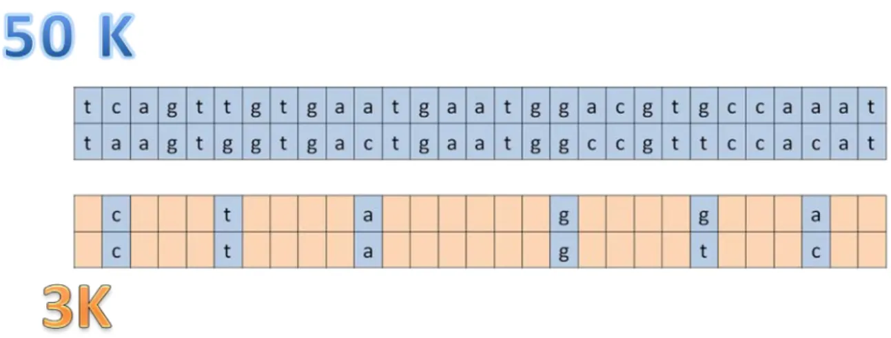
Imputation requires 2 distinct data sets, including genotypes of different individuals and corresponding to 2 different marker panels (Figure 2). Some markers are usually included in both panels in order to create a link between the 2 data sets (actually, the more markers in common, the more accurate the imputation). Pedigree information (relationships between individuals) and the genetic marker map (position of markers on the genome) bring additional information.

Figure 2 Diagram describing imputation. The rows correspond to sequences of bases (a,c,g,t) on the paternal and maternal haplotyes. Imputation consists in filling in the gaps (in orange here) of the low density using information extracted from high density

(23)

1-1.4. STATISTICAL BASIS OF IMPUTATION

Imputation usually relies on hidden Markov model. A Markov model is a stochastic process that assumes that the conditional probability distribution of future states depends only upon the present state.

Let us consider a series of markers present on a given chromosome segment and distributed according to their position on the genetic map. The Markov property implies that only the information at a marker n is required to impute the genotype at marker n+1.

Figure 3 A hidden Markov model. c0, c1, ... cT follow the Markow property : to determine c3, only the information at c2 is necessary. In the case of hidden Markov model, c0 to cT are not observable. y0, y1 ... yT represent the observation. Observation y 3 only relies on the hidden state of c3.

Instead of directly considering the measurable variable (here the genotype), we consider a hidden variable which could correspond to ancestors’ haplotypes following the Markov property. When we deal with SNP, the information at each single marker is binary, so it is very limited. Allowing a larger number of different states at every position gives more flexibility to the statistical tool to sum up the information corresponding to the previous positions. For a given position at a locus n, a hidden state is assigned based on the information gathered in the hidden state at the position n-1. This hidden state (the haplotype for instance) at position n corresponds to one state of the observed variable (here the genotype) at position n.

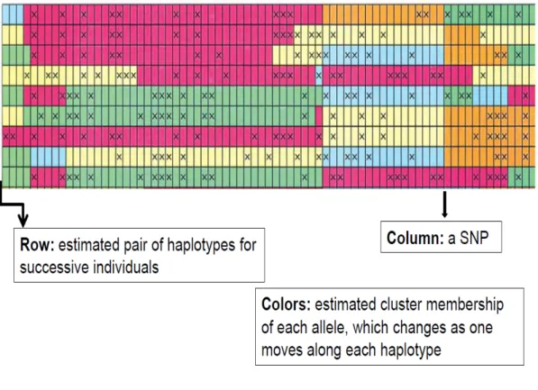
During the process of imputation, hidden Markov model usually creates a mosaic structure (see Figure 4).

(24)

Figure 4 Mosaic structure obtained with an imputation software based on a hidden Markov model (from Scheet and Stephens, 2006). For each individual correspond 2 rows (diploid organisms). And every marker is represented by a column. The color of each spot refers to the hidden state. X correspond to one allele of the SNP when blank correspond to the other allele, defining the observed variable (i.e. the genotype). Colors can be seen as ancestors’ haplotypes.

1.2. The different imputation software

1-2.1. THE FIRST EXPERIENCE OF IMPUTATION IN HUMAN GENETICS WAS BASED ON POPULATION LINKAGE DISEQUILIBRIUM

As often in genetics, human genetics are a few steps ahead. As the first genome to be sequenced, the human genome was studied using different SNP chips. In order to aggregate data coming from different studies, the need for imputation arose. The main focus while using genomic data in human genetics is association studies. Most of the time, the aim is to find a causal mutation in a gene involved in a specific disease. The data includes individuals from small families (compared to large half-sibs families encountered in dairy cattle) and may

(25)

come from sub-populations usually not related to each other. For these reasons, imputation is based on the linkage disequilibrium observed at the population level.

Two software specifically dedicated to imputation of human data are briefly presented here. There exist many more but these two became standards and are heavily used worldwide. The first one is fastPHASE, developed by Scheet and Stephens (2006), derived from PHASE (Stephens et al. 2001) allowing the analysis of larger data sets. It is based on a hidden Markov model. The idea is that over short regions, haplotypes tend to cluster into groups. The model specifies a given number K of unobserved states (cluster of haplotypes). The mosaic structure seen in Figure 4 is produced by fastPHASE. Colours can be seen as founders’ haplotypes segregating in the population. The software can be used for both haplotyping and imputation. For imputation, the best guess is sampled from the conditional distribution of the observed genotype given the hidden state. Haplotyping consists in allocating the paternal or maternal origin of a given chromosome segment.

The second one is Beagle, developed by Browning and Browning (2007) and heavily used in the field. It is also based on an hidden Markov model. It has some similarities with fastPHASE, the main difference being that the haplotype-cluster model is localized. While the number K of unobserved states is required as an input in fastPHASE, and remains the same all along the chromosome, this value can differ for every marker position in Beagle. A Directed Acyclic Graph (DAG) is produced and summarizes the LD pattern. It gives the different emission probabilities from one hidden state at one marker position to the possible hidden state at the next position (see Figure 5). The DAG (which can be seen as a special kind of tree where branches can merge) is simplified using the Viterbi algorithm. In Beagle theory, recombination is modeled as merging edges.

(26)

Figure 5 Example of a DAG representing localized-cluster model for 4 markers. For each marker allele 1 is represented by a solid line and allele 2 by a dashed line. From Browning and Browning (2007)

Note: The Viterbi algorithm, initially developed to remove noise in communication, is also used in bio-informatics nowadays. It allows to simplify a tree -such as a hidden Markov model, or here, the DAG- while constructing it, matching similar edges.

There exist many other software, such as IMPUTE (Marchini et al. 2007), and several are well described in a review from Marchini and Howie (2010).

1-2.2. IMPUTATION SOFTWARE SPECIFICALLY DEDICATED TO ANIMAL POPULATIONS, BASED ON LINKAGE AND MENDELIAN SEGREGATION RULES

Human population and livestock populations are much different (in terms of LD for instance) but the data sets built for genetics studies are even more different. For both species they are based on SNP data. But human SNP chips include many more markers (usually around one million of SNP) while livestock population are studied with medium density SNP chip (dozens of thousands SNP). The main difference consists in the “depth” of the pedigree. Human genetic data sets are usually built on small families or even unrelated individuals. On the other hand, genetics data sets of livestock populations are usually formed of related individuals across several generations. For example, in dairy cattle, very large half-sibs families are studied across several generations.

Considering these differences, some geneticists specialized in animal populations developed specifically dedicated software that take advantage of the very specific family structure of livestock populations. Indeed, when one or both parents are genotyped, some specific rules can be applied in order to partially determine with certainty the genotype of the offspring.

(27)

Those rules are based on Mendelian segregation. The simplest example is when the sire is homozygous at one locus. One knows for sure the paternal allele of the offspring.

Druet et al. (2008) described such a strategy. The software, which was not publicly released at first (it is now included in a package) is called linkPHASE. It follows 4 different steps. First, homozygous alleles are assigned to both (paternal and maternal) phases. Then, markers that can be unambiguously determined (based on homozygous markers of parents for instance) also are assigned. Then anchoring markers (heterozygous markers for parents for which phases offspring phases are already determined) are defined. They are used as informative flanking markers. Emission probabilities are then computed based on genetic distances. Finally, the most probable haplotypes are assigned if they reach a given probability threshold (95%). This method is very fast, and takes full advantage of the family structure of livestock data sets.

linkPHASE fastPHASE or Beagle

developed for livestock populations human population

data usually used large half-sibs families unrelated individuals

account for linkage LD (linkage disequilibrium)

based on

Mendelian segregation rules

and informative flanking markers hidden Markov model markers it was initially

developed for

microsatellites

(multi-allelic) SNP (bi-allelic)

accuracy medium to high

excellent at high density

speed very fast

slow (especially when data includes

thousands of individuals) Table 1 Main differences between linkPHASE and fastPHASE/Beagle

(28)

1-2.3. COMBINING THE 2 SOURCES OF INFORMATION: POPULATION BASED LINKAGE DISEQUILIBRIUM AND LINKAGE USING FAMILY INFORMATION

Both approaches (hidden Markov model based on population LD in human genetics and mendelian segregation rules and linkage based on family structure in livestock populations) are not exclusive. Traditional human genetics approaches can be used to impute livestock SNP data. However they are slow. Moreover, it is a pity not to take into account simple Mendelian segregation rules to determine unambiguously an important fraction of the genotypes to be imputed. Accounting for family information can also avoid some errors when the parent carry rare haplotypes in the population. Druet and Georges (2010) proposed a method to combine these 2 sources of information. It is included in a package called PHASEBOOK. In the imputation process they proposed, Mendelian segregation rules first are applied. Depending on the value of the probability threshold, linkage information can be used to assign the most probable haplotype for some regions (given informative flanking markers). This is done with the linkPHASE software and partially reconstructed genotypes are obtained. Then either the fastPHASE probability model or the Beagle probability model are used (with some modifications) to exploit linkage disequilibrium. This is performed using programs called dualPHASE or DAGphase. For instance, DAGphase exploits the DAG created by Beagle on a base population. To sum up and simplify, this method is very similar to a regular hidden Markov model (as used in human genetics). The main difference is that the input file includes genotypes partially reconstructed using family information. It is a way to speed up the process with no loss in accuracy since only genotypes assigned with certainty are added.

There exist other kinds of methods to perform imputation. One can think of long range phasing. Initially proposed by Kong et al. (2008), it considers that long identity by descent blocks may be inherited from a hypothetical common ancestor, even for unrelated individuals. In practice, “libraries” of long haplotype blocks are created based on genotypes of the training population. Hickey et al. (2011) proposed such an approach adapted to dairy cattle populations with a software called Alphaimpute. One possible drawback is that some of these software leave some missing markers uncalled. Depending on the genomic evaluation method used, this downside may unable the use of such an imputation method. Such software were not studied in this document. Johnston et al. (2011) compared several different software on dairy cattle data. Long range phasing methods are more recent and one may consider that they

(29)

are really promising. One could find a way to combine this approach with other sources of information in order to speed up the process and to increase even more accuracy.

Findhap is a software developed by VanRaden et al. (2011) that combines pedigree reconstruction of genotypes and population haplotyping. It uses libraries where long block of haplotypes are sorted according to their frequency in the training population, and checks whether the most frequent haplotypes fit with the low density genotypes and nearby markers in order to impute missing SNP.

Imputation clearly appears as a very interesting approach: it fully benefits from the links (either at the population or the family level) that exist between individuals genotyped at the various densities to predict complete genotypes from lower density genotypes at a reduced cost.

1.3. Measures of imputation accuracy

There are two kinds of methods to assess imputation accuracy. The first one is to double genotype the same individuals. The animals are genotyped on both the low density and high density chips and imputed SNP are compared with real ones. The main advantage of such a method is that it is the most realistic, and it accounts for both genotyping and imputation issues. However this technique has two main drawbacks: first it is more expensive (2 genotypes per animal). Second, it requires that the studied chip already exist technically, whereas sometimes, one just want to test a given set of markers to determine what the imputation accuracy would be if such a chip were developed.

For these reasons, another way to measure imputation accuracy is to simulate in silico low density genotypes. Only high density genotypes are used. Then, a low density genotype is created by erasing markers that are not present on the low density chip (but present on the initial high density chip). It is possible to test as many different chips as required. Differences observed between imputed and real genotypes only result from imputation mistakes and are not due to genotyping errors of common markers of the 2 chips.

(30)

• Direct measures obtained only comparing true and imputed genotypes.

The advantage of simulation study is to know the “true” genotype for a given marker, present on the high density chip, and missing on the low density chip. The genotypes obtained after imputation can be compared with this “true” genotype.

1-3.1. ERROR RATE OR CONCORDANCE RATE

The easiest measure of imputation accuracy is to count the number of markers for which true and imputed genotypes differ. This number, divided by the total number of missing markers, gives a ratio, usually expressed in %, called the imputation error rate.

This measure was used by e.g. Zhang and Druet (2010), Dassonneville et al. (2011).

Simply derived from the error rate, the concordance rate relates to the proportion of missing markers that were correctly imputed, meaning the number of missing markers for which true and imputed genotypes are the same divided by the total number of missing markers.

The concordance rate appears to be a more optimistic way of presenting the same result: 95% of markers correctly imputed sounds better than 5% of markers incorrectly imputed.

This measure was used by e.g. Weigel et al. (2010), Dassonneville et al. (2012).

One can easily get the concordance rate from the error rate figures (or the other way around) as:

concordance rate = 100 – error rate (or 1 - error rate when not expressed in%).

1-3.2. COUNTING PER GENOTYPE OR PER ALLELE

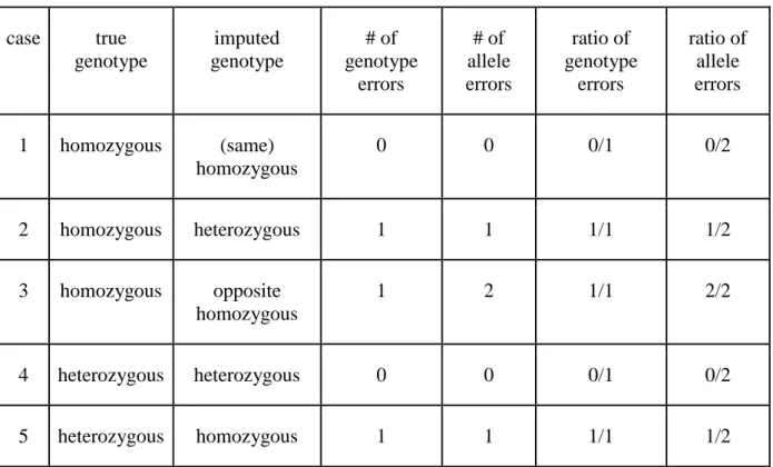
There are 2 ways of considering imputation results (or genotyping results) for a given marker: ● Considering the genotype

During the genotyping procedure, fluorescence is used to assign individuals’ genotypes for a given SNP to 3 clusters, corresponding to the 2 different homozygous possibilities, and one for the heterozygous. One possible way of measuring imputation is to check whether the genotype was properly assigned after imputation to the correct group. Easily, and as stated in Table 2, if the imputed and true genotypes are different, then the imputed genotype is considered as wrong.

(31)

● Considering the 2 alleles

One may also consider that the genotype for one locus actually hides 2 separate sources of information corresponding to the 2 different alleles (inherited from the 2 parents). One imputed allele (of one haplotype, either the paternal or the maternal one) may be right while the other one may be wrong. Considering either the 2 right or the 2 wrong as one error may appear simplistic then.

case true genotype imputed genotype # of genotype errors # of allele errors ratio of genotype errors ratio of allele errors 1 homozygous (same) homozygous 0 0 0/1 0/2 2 homozygous heterozygous 1 1 1/1 1/2 3 homozygous opposite homozygous 1 2 1/1 2/2 4 heterozygous heterozygous 0 0 0/1 0/2 5 heterozygous homozygous 1 1 1/1 1/2

Table 2 genotype and allele error rates for all the different cases which can be observed when comparing true and imputed genotype.

Obviously, when imputation is correct, i.e. when true and imputed genotypes are identical (cases 1 and 4 in the table), the error rate is 0 and both genotype or allele measures are identical. We expect this situation to be the most frequent.

When the true genotype is homozygous and the imputed genotype is heterozygous, or vice-versa (cases 2 and 5), the error rate is 1 for the genotype measure, and ½ for the allele measure. It is the main difference between the 2 measures. This situation is expected to be the main source of errors.

(32)

When true and imputed genotypes are opposite homozygous (case 3), the error rate is 1 for both measures. However, if the error rate p is small, the probability of such an error is even smaller, as it is proportional to p².

Considering the last situation as rare, one can approximate the genotype error rate as twice the allele error rate. This approximation can be used to “translate” results from one study to be compared with another one.

Some authors (e.g. Weigel et al., 2010) prefer to use genotype error rate. They argue that allele error rate is a way to present better results, as the error rate appears lower (or concordance rate appears higher). As Druet et al. (2010), we chose to consider the allele error rate. Imputed genotypes will be used in genetic evaluations, which are based on an additive model. For this reason, if the imputed genotyped for one marker is half correct (cases 2 and 5), we can expect the resulting genomic evaluation as half right, and not completely wrong. This is the reason why we prefer to use allele error rate.

1-3.3. CORRELATION BETWEEN TRUE AND IMPUTED GENOTYPES

Most of the authors report concordance or error rates, based on alleles or genotypes. These measures are simple to calculate, and easily derived from the other one. There exist some alternative measures that present some better properties. Hickey suggested to use correlation between true and imputed genotypes in order to account for MAF.

As we stated in part 2.1. , “Using concordance rate as imputation efficiency criterion may be misleading as it depends on MAF. The lower the MAF, the higher the concordance rate, for the same efficiency and this should be accounted for in the interpretation. For example, with an average MAF of 0.2, 80% of the results would be correct after random sampling of the missing alleles. Getting a 95% concordance rate corresponds only to a 75% ( = (95-80)/(100-80) ) imputation efficiency. Correlations are an alternative criterion less dependent on MAF.“ One hidden message is that, a marker with low MAF presents less variation across individuals, bringing less information to the genomic model, therefore good concordance rate for such marker is misleading when one wants to predict the information brought from imputed genotypes to the evaluation model. In the study of Hickey et al. (2012), performed on maize data, they plotted both concordance rate and correlation as a function of MAF (Figure

(33)

6). One may thereby observe differences between the 2 measures, low MAF markers present high concordance rate but low correlation.

We chose to report the 2 kind of measures.

Figure 6 (from Hickey et al. 2012) 2 measures of imputation accuracy depending on MAF of markers. On the graph on the left is represented the concordance rate whereas on the right is presented the correlation.

1-3.4. COMPARING PHASES OR GENOTYPES ?

The French genomic evaluation model relies on haplotypes (Boichard et al., 2012). These haplotypes are derived from the phased genotypes obtained after imputation. One may want to measure imputation accuracy looking at the phases produced. However it is very difficult to compare phases outputs. For the same genotypes, it is possible to count the number of switches (Druet, personal communication), i.e. the number of apparent recombinations on the imputed phase but not present on the “true” phase. An additional drawback is that this measure requires to “know” the “true” phases. But phases can only be obtained from genotype data after running a phasing software (and this software may also induce some errors).

(34)

1-3.5. MEASURING CONSEQUENCES OF IMPUTATION ERRORS ON GENOMIC EVALUATIONS

• Graphical representation of G matrices - The G matrix

Many countries (ref) have chosen the GBLUP approach to implement genomic evaluation. One possibility is to use a G matrix as in VanRaden (2009). Every line/column corresponds to an individual, and based on marker information, a “genomic relationship” is calculated between every 2 individuals. Then, this G matrix can be used within the mixed model equations as if it were the A matrix (which is based on pedigree relationships).

- The G matrix as a measure of imputation accuracy

When one wants to compare genomic evaluations based on true or imputed genotypes using the GBLUP method, the G matrix has first to be derived. Zukowski (personal comunication) propose to directly compare G matrices (either the “true” one or the one based on imputed genotypes). Figure 7 proposes a graphical representations of the G matrices obtained with several imputation methods. Graphical representations are not as easy to compare as numerical values. However, they give a nice and quick overview. It is also to measure distances between matrices.

(35)

Figure 7 graphical representations of the G matrices obtained with several imputation methods (from Zukowski) The top matrix only represent relationships between individual of the training population (before imputation). The matrix in the middle is the “true” G matrix. The top left matrix has been computed after random imputation (RAN) of the missing markers for the validation population. The matrix down on the left is obtained after imputation based on family structure (FAM, Wimmer et al., 2012). The 2 matrices on the right are obtained after imputation of missing markers using ChromoPhase.f90 (CHR1 and CHR2, Daetwyler et al., 2012). The matrix on the bottom (BEA) is based on imputed genotypes performed using Beagle software.

With no surprises, random imputation gave poor results but can be considered as a “control”. Chromophase and Beagle gave the best imputation accuracy figures (results not shown). However, comparing graphical representations clearly shows that the matrix most “similar” to the “true” G matrix is the one obtained after Beagle imputation.

While here we want to predict relationships between individuals, Beagle which is only based on population linkage disequilibrium (and does not take into account complex pedigree relationships) clearly better predicts “genomic relationships” between individuals. This illustrates how well Beagle works, and is consistent with the better imputation of genotypes of individuals closely related to the reference population.

(36)

1-3.6. COMPARING GENOMIC EVALUATIONS BASED ON IMPUTED GENOTYPES

In animal breeding, the main use of imputed genotypes is to include them in genomic evaluation. Obviously, the best way to measure the consequences of using imputed genotypes on genomic selection is to run genomic evaluations on both imputed and true genotypes and compare the DGV or GEBV obtained. Phenotypes and complete genotypes of the training population are used, as well as imputed genotypes for the validation population. Genomic breeding values based on imputed and true genotypes can be compared. Moreover, they can be compared to phenotypes (DYD or deregressed proofs of validation animals). One can then estimate the loss in reliability when using imputed genotypes instead of true genotypes.

(37)

1.4. Article I Impact of imputing markers from a low density

chip on the reliability of genomic breeding values in Holstein

populations

1-4.1. BACKGROUND

In 2010, Illumina developed a new genotyping tool : the Bovine 3K Beadchip ® based on the GoldenGate technology (GG 3K). The cost of this SNP chip was reduced by 68% compared to the standard Bovine SNP50®. This did not mean that the total genotyping cost was substantially reduced since lab costs remained more or less the same. The main target of this product was the large population of females. The use of a cheap tool was thought to be crucial to launch female genotyping as a new service.

Also in 2010, a European consortium, Eurogenomics, was formed. It covered 4 large Holstein populations (Dutch-Flemish, French, German and Nordic - Denmark, Finland, Sweden -). Its members decided to join their reference population (15,966 progeny-tested genotyped bulls) in order to achieve more reliable genomic predictions. Their scientific partners also decided to cooperate in order to conduct common studies. This article is one of such studies.

1-4.2. OBJECTIVES

The purpose of the study is to measure imputation accuracy and to quantify the loss in reliability when using imputed genotypes instead of real genotypes. The aim is to determine whether such a low density tool can be used in practice.

The novelty of the paper (among others studies on imputation) lies on the fact that genomic evaluations based on imputed genotypes were calculated and their quality was compared to the situation without imputed genotypes. That was done using 2 different methods for genomic prediction (GBLUP in Nordic countries, GMAS in France) considering 4 different traits. It was also desired to compare the loss in reliability due to the use of low density panels to the gain achieved when increasing the reference population size.

(38)

Article I

Dassonneville R., R.F. Brøndum, T. Druet, S. Fritz, F. Guillaume, B.

Guldbrandtsen, M.S. Lund, V. Ducrocq, G. Su. 2011

Impact of imputing markers from a low density chip on the

reliability of genomic breeding values in Holstein populations

(39)

ABSTRACT

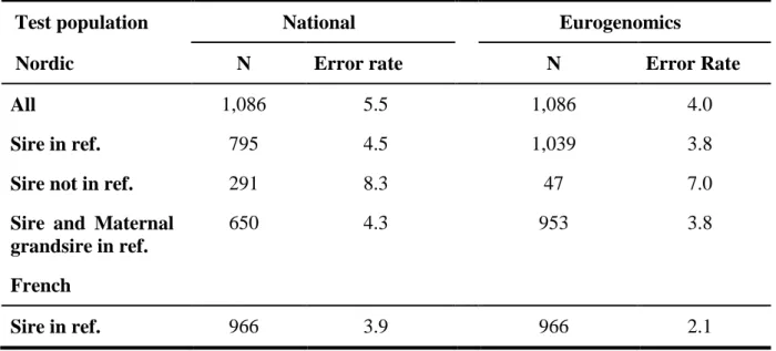
The purpose of this study was to investigate the imputation error and loss of reliability of direct genomic values (DGV) or genomically enhanced breeding values (GEBV) when using genotypes imputed from a 3K single nucleotide polymorphism (SNP) panel to a 50K SNP panel. Data consisted of genotypes of 15,966 European Holstein bulls from the combined EuroGenomics reference population. Genotypes with the low density chip were created by erasing markers from 50K data. The studies were performed in the Nordic countries (Denmark, Finland, and Sweden) using a BLUP model for prediction of DGV and in France using a genomic marker assisted selection approach for prediction of GEBV. Imputation in both studies was done using a combination of the DAGPHASE 1.1 and Beagle 2.1.3 software. Traits considered were protein yield, fertility, somatic cell count and udder depth. Imputation of missing markers as well as prediction of breeding values were performed using two different reference populations in each country; either a national reference population or a combined EuroGenomics reference population. Validation for accuracy of imputation and genomic prediction was done based on national test data. Mean imputation error rates when using national reference animals was 5.5% and 3.9% in the Nordic countries and France, respectively, whereas imputation based on the EuroGenomics reference dataset gave mean error rates of 4.0% and 2.1%, respectively. Prediction of GEBV based on genotypes imputed with a national reference dataset gave an absolute loss of 0.05 in mean reliability of GEBV in the French study, whereas a loss of 0.03 was obtained for reliability of DGV in the Nordic study. When genotypes were imputed using the EuroGenomics reference a loss of 0.02 in mean reliability of GEBV was detected in the French study, and a loss of 0.06 was observed for the mean reliability of DGV in the Nordic study. Consequently, the reliability of DGV using the imputed SNP data was 0.38 based on national reference data, and 0.48 based on EuroGenomic reference data in the Nordic validation, and the reliability of GEBV using the imputed SNP data was 0.41 based on national reference data, and 0.44 based on EuroGenomic reference data in the French validation.

(40)

INTRODUCTION

Genomic selection (Meuwissen et al., 2001) is becoming a routine tool for genetic evaluation in dairy cattle breeding. Currently, an SNP panel with 54,000 markers is widely used. A new low density panel with only 3,000 markers at a lower price potentially reducing genotype costs is now also available (Illumina, San Diego). Using the low density panel instead of the current one may allow cattle breeders to genotype more bulls and cows.

Several options for selecting a low density panel have been suggested. One option is to select a number of markers with large effects for a given trait, another is to use markers evenly spaced across the genome. Previous studies showed that the difference in reliability of the genomic breeding values, when using 3,000 markers with large effect or 3,000 markers evenly spread across the genome, is small (Moser et al., 2010). The option of evenly spaced markers removes the need for trait and breed specific low density SNP panels. The efficiency of a trait specific marker panel also depends on the linkage disequilibrium (LD) between the markers with large effect and the actual QTL. This LD might decline through generations. The other advantage of evenly spread markers is the possibility to use statistical methods to impute the missing markers, thus extending the 3,000 markers to 50,000 markers albeit with some uncertainty. This is also possible with unevenly spread markers, but then the accuracy of imputation is expected to be lower.

It has been reported that a lower marker density leads to lower reliability of genomic prediction (Moser et al., 2010). A feasible strategy is to extend the low density markers to the current 50K markers by imputation. Several methods for imputation of SNP markers, relying on either linkage based on family information (Daetwyler et al., 2010) or LD based on population information (Browning and Browning, 2007; Scheet and Stephens, 2006), have been proposed. It is also possible to combine both types of information (Druet and Georges, 2010). In a study using this combined approach to impute from 3,000 to 50,000 markers, where the 3,000 markers were specially selected for high minor allele frequency, Zhang and Druet (2010) found an allele error rate, i.e. the proportion of incorrectly predicted alleles, of approximately 3%. A study by Weigel et al. (2010) on American Jersey cattle has shown that using 3,000 SNPs for candidates imputed to a 50K SNP panel can provide approximately 95% of the predictive ability achieved using the real 50K SNP panel.

The accuracy of imputation can be increased by increasing the size of the reference population. EuroGenomics is a collaboration between four European AI companies and

(41)

scientific partners: DHV-VIT (Germany), UNCEIA-INRA (France), CRV (Netherlands, Flanders) and Viking Genetics-Aarhus University (Denmark-Finland-Sweden). The collaboration includes the sharing of reference populations for genomic selection, where each country initially contributed 4,000 genotyped Holstein bulls with progeny tested breeding values. A previous study showed a significant increase in reliability of genomic breeding values using this combined reference population (Lund et al., 2010). We expect that the accuracy of imputation based on EuroGenomics reference data will be higher than that based on national reference data.

The objective of this study is to investigate the imputation error, when imputing from a 3K SNP panel to a 50K SNP panel using a group of reference animals with 50K information. The 3,000 markers were the same as the Illumina 3K SNP panel. The imputed SNP markers were used for genomic prediction to assess how the imputation error rate affects the reliability of genomic breeding values and the ranking of the animals. This assessment was carried out in the Nordic countries and France. For both analyses, a validation population consisting of national test animals with 3K genotype was imputed to 50K genotype using a reference population made of either national or EuroGenomics data.

MATERIAL AND METHODS

DATA

The combined EuroGenomics reference population contains 15,966 progeny tested bulls with genotypes from the Illumina Bovine 50K SNP panel (Matukumalli et al., 2009). 4,000 Dutch bulls were genotyped using a customized CRV 60K chip, but by double genotyping 972 influential bulls with the Illumina 50K chip, it was possible to impute markers from the Illumina chip for all Dutch bulls with an imputation error of less than 1% (Druet et al., 2010). Measurement of imputation error rate and reliability of genomic predictions for Nordic and French bulls were carried out separately, using either national or EuroGenomics reference data. Deregressed proofs (DRP) on the scale of the target population calculated from Interbull 2010-01 MACE proofs were used for predicting and validating DGV and GEBV, if the equivalent daughter contribution (EDC) was at least 20 (Lund et al., 2010). In the French study, daughter yield deviations (DYD) from the October 2009 national evaluation were used as phenotypes for the French bulls. The reference and validation populations were divided

(42)

according to the bulls’ birth date. The cut-off dates were October 1, 2001 and June 13, 2002 in the Nordic and French case, respectively. Thus, about 25% of national genotyped bulls were taken as a validation set.

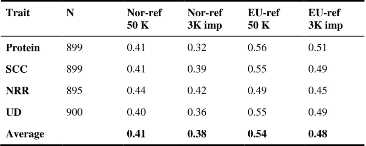
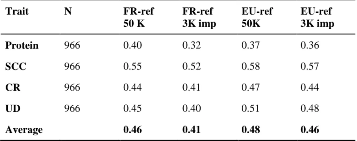
The traits studied were protein yield, somatic cell count (SCC), fertility (defined as non return rate (NRR) in the Nordic countries and conception rate (CR) in France), and udder depth. Heritabilities and number of animals available for the specific traits are shown in Table 1.

Table 1: Heritabilities (h²) and number of animals used for protein yield, somatic cell count (SCC), fertility and udder depth (UD) in the Nordic and French study.

Nordic French Trait h² Nordic reference Euro reference Nordic validation h² French reference Euro reference French validation Protein 0.39 3,038 10,701 899 0.3 3,071 12,078 966 SCC 0.15 3,077 10,800 899 0.15 3,071 12,078 966 Fertility 0.02 3,069 10,712 895 0.02 3,071 12,078 966 UD 0.37 2,958 10,755 900 0.36 3,071 12,078 966

Marker data were edited according to procedures used in Nordic countries and in France.

Nordic marker editing:

The genotypic data was edited both per animal and per locus. At the animal level, the requirements were a call rate above 95% except for some old animals which were accepted with call rates of at least 85%. Marker loci were accepted, if they had a call rate of at least 95% in a large reference sample. Loci with a minor allele frequency less than 5% were excluded. Loci without a known map position in the Btau 4.0 assembly or mapped on the X chromosome were discarded. Animals with an average Gen Call score (Illumina, 2005) of less

(43)

than 0.65 were excluded. Individual marker typings with a Gen Call score of less than 0.6 were also discarded.

French marker editing:

The French genotypic data was first edited per locus. Markers without a known map position in the Btau 4.0 assembly, or mapped to the X-chromosome were removed. Markers were then filtered for Hardy Weinberg equilibrium (q value < 0.01). Markers with call rates below 0.85 were removed. Markers with MAF strictly equal to 0 were removed. Genotype data were finally checked for Mendelian inconsistencies between parents and offspring. Inconsistent genotypes were set to missing. Marker editing procedures differed slightly between France and the Nordic countries (including Gen Call score for example).

While checking for inconsistencies between parents and offspring, Mendelian segregation rules were also applied in order to determine marker types of ungenotyped ancestors. Inferred marker data was not complete. However, it is important for ancestors with large numbers of progeny. Thus, the French national training population included 3,071 animals with real observed marker types (Table 2) and a total of 3,505 when ancestors with imputed genotypes are included. The corresponding figures for the EuroGenomics population are 12,078 and 13,947 animals, respectively. This might help for further imputation, especially through linkage information.

Table 2: Number of animals and number of markers used.

National EuroGenomics No. of Markers

Reference Validation Reference Validation Reference Validation Nordic 3,058 1086 10,880 1,086 38,545 2,285 France 3,071/ 3,505* 966 12,078/ 13,947 * 966 43,582 2,635

(44)

Simulating Illumina Bovine 3K Bead Chip Data

The 2900 SNPs in the Illumina Bovine 3K Bead chip are all included in the Bovine 50K chip (except for 14 markers located on the Y-chromosome). To mimic the low density chip, marker types of test animals, i.e. animals born after the cut-off date, were obtained by erasing markers from the 50K marker type (i.e. in silico chip). As 3K genotypes are simulated from 50K data, they do not account for a possibly higher genotyping error rate with the 3K chip. After marker editing as outlined above, 2,285 and 2,635 markers were kept for the Nordic and French data, see Table 2.

Imputation of missing SNP markers

Imputation of markers was done using the PHASEBOOK package (Druet and Georges, 2010) in combination with Beagle 2.1.3 (Browning and Browning, 2007). The method was applied as a stepwise procedure using both linkage and LD information. The same procedure as in Zhang and Druet (2010) was applied. First, all markers that can be determined unambiguously using Mendelian segregation rules were phased using the LinkPHASE software. In the first step, both training and test animals were included. An iterative procedure was then applied, where a directed acyclic graph (DAG) describing the haplotype structure of the genome was fitted to the partially phased data from the previous step. This was, however, only done for the reference animals. This was done for 10 iterations and then, the final DAG, the genotype file and the output from LinkPHASE (partially phased data) were used to reconstruct haplotypes and impute missing markers for both test and training animals using the Viterbi algorithm. With Beagle and PHASEBOOK, all markers are imputed, and the method does not leave any missing markers. More details on the imputation procedure can be found in Druet et al. (2010) and Zhang and Druet (2010).

Allele imputation error rate calculation

The number of errors was counted as 0 when the imputed and observed marker types were identical, 1 if the real marker type was homozygous and the imputed genotype was heterozygous (or vice versa), and 2 if real and imputed marker types were opposite