HAL Id: pastel-00000944
https://pastel.archives-ouvertes.fr/pastel-00000944
Submitted on 3 Feb 2005
HAL is a multi-disciplinary open access
archive for the deposit and dissemination of sci-entific research documents, whether they are pub-lished or not. The documents may come from teaching and research institutions in France or abroad, or from public or private research centers.
L’archive ouverte pluridisciplinaire HAL, est destinée au dépôt et à la diffusion de documents scientifiques de niveau recherche, publiés ou non, émanant des établissements d’enseignement et de recherche français ou étrangers, des laboratoires publics ou privés.
Interpolation et rééchantillonnage de données spatiales
et application à la cartographie urbaine et à la
détermination du fond cosmique primordial
Svitlana Zinger
To cite this version:
Svitlana Zinger. Interpolation et rééchantillonnage de données spatiales et application à la cartographie urbaine et à la détermination du fond cosmique primordial. domain_other. Télécom ParisTech, 2004. English. �pastel-00000944�
Th`ese
pr´esent´ee pour obtenir le grade de docteur
de l’Ecole Nationale Sup´erieure des T´el´ecommunications
Sp´ecialit´e: Signal et Images
Svitlana Zinger
Interpolation et r´e´echantillonnage de donn´ees
spatiales et application `
a la
cartographie urbaine et `
a la d´etermination
du fond cosmologique primordial
Composition du Jury:
Bernard Chalmond
Rapporteur
Annick Montanvert
Rapporteur
Laure Blanc-F´eraud
Examinateur
Jacques Delabrouille
Examinateur
Michel Roux
Examinateur
Acknowledgements
I would like to express my gratitude to the director of my thesis, Professor Henri Maˆıtre who provided me this great opportunity to work towards a Ph.D. degree at one of the best institutes of France. I appreciate very much his constant support and attention during all my time in ENST. His help and encouragement were crucial for my thesis. I am also thankful to Michel Roux, the co-director of my thesis, for all his help and practical advices that made my progress faster and easier.
I would like to thank to the members of the jury of my thesis. I thank Professors Bernard Chalmond and Annick Montanvert for writing reports on my thesis and their suggestions. The comments of Annick Montanvert helped me very much to improve the text of my thesis. I appreciate her help very much. I thank very much to Laure Blanc-F´eraud and to Jacques Delabrouille for accepting to participate in the jury of my thesis. I am especially thankful to Jacques Delabrouille for providing me the cosmic microwave background data, for discussions and suggestions on this topic.
I am thankful to Olivier de Joinville for providing me the laser scanning data and for helping me to understand it. Many discussions with Mila Nikolova, Evgeniy Pecherskiy, Yann Gousseau made me realize the theoretical issues of cost function based methods and minimization problems. I thank them very much.
I would like to convey my feelings to all the TSI faculty members, postdoc fellows, Ph.D. students (Jasmine, Yong, C´eline, Carlos, Eve, Daniel, Alejandro, Tony, Dalila, Saeid, David, Antonio and others). It was my pleasure to work and communicate with them.
Abstract
In this thesis we study interpolation methods for irregularly distributed spatial data. We consider the resampling problem applied to the altimetry measures on an irregular grid obtained by airborne laser scanning. This type of data is irregularly spaced and a resampling on a regular grid is necessary in order to generate a digital elevation model (DEM). Some well-known methods are considered: linear triangle-based interpolation, nearest neighbor interpolation, and kriging. We propose an energy minimization ap-proach which allows to avoid the drawbacks of the methods mentioned above. This approach imposes a model of a surface that corresponds to urban areas. The energy function is adapted for irregularly distributed data. The methods are tested on two sets of irregularly distributed spatial points acquired by a laser scanner on Brussels and Amiens. These data sets have different sampling patterns and therefore let us better analyse the performance of the methods. We also applied these methods as well as binning for determination of cosmic microwave background.
R´
esum´
e
Les probl`emes d’interpolation sont fondamentaux dans de nombreux domaines des sciences appliqu´ees, en particulier en traitement du signal et des images. L’av`enement des technologies num´eriques a en effet contribu´e au d´eveloppement de techniques de mesure fournissant des valeurs discr´etis´ees des signaux `a acqu´erir. Il apparaˆıt capital de disposer de m´ethodes d’interpolation adapt´ees `a la physique du signal, et donc `a l’´eventuelle irr´egularit´e spatiale des grilles discr`etes repr´esentant ces mesures. Dans ce cadre, un mod`ele a priori du signal est souvent utile.
Si de nombreuses m´ethodes de traitement d’image sont bien connues pour les traitements de donn´ees construites sur une grille r´eguli`ere, il n’en est pas de mˆeme pour les donn´ees sur grille irr´eguli`ere et sur grille avec gigue. Ces types de grilles se rencontrent en particulier en t´el´ed´etection : bien que, dans le meilleur des cas, les mesures soient r´eguli`erement ´echantillonn´ees dans le r´ef´erentiel du capteur, les points 3D g´eor´ef´erenc´es correspondants sont irr´eguli`erement espac´es dans le r´ef´erentiel ter-restre. L’interpolation et le r´e´echantillonnage des donn´ees originales sur une grille r´eguli`ere permettent de les traiter et de les analyser. En effet, des traitements tels que la visualisation, la segmentation, la fusion, etc. n´ecessitent souvent d’avoir une grille r´eguli`ere.
Le nombre important de techniques d’interpolation disponibles aujourd’hui se r´eduit consid´erablement lorsque l’on veut interpoler des valeurs distribu´ees sur une grille irr´eguli`ere. C’est la probl´ematique que l’on consid`ere dans le cadre de cette th`ese. Nous traiterons en particulier la question complexe de l’interpolation d’un signal `a bande non limit´ee et dont les mesures sont dispers´ees dans l’espace. Cette question est envisag´ee `a partir de donn´ees du lev´e laser a´eroport´e acquises sur des zones urbaines. En effet, dans les zones urbaines, les bords des bˆatiments forment des discontinuit´es conduisant `a un signal `a bande non limit´ee.
La cr´eation de mod`eles 3D de villes est importante pour plusieurs raisons. Elle per-met par exemple la cr´eation et la mise `a jour des syst`emes d’information g´eographiques, la planification urbaine et les projets de d´eveloppement cens´es empˆecher la disper-sion des substances polluantes, ou encore la planification de r´eseau de transport et le positionnement des antennes de t´el´ecommunication. La t´el´ed´etection sur des zones urbaines est un des outils permettant de construire les repr´esentations des villes en r´ealit´e virtuelle 3D. Cette technique autorise, par lev´e laser a´eroport´e, une acquisition rapide et pr´ecise de donn´ees en cours de test sur des zones urbaines. Dans la premi`ere partie de cette th`ese, nous nous int´eressons `a cette technique en pr´esentant l’´etat des recherches qui la concernent. Ceci nous permet de comprendre la nature des donn´ees
acquises, notamment en ce qui concerne le bruit et la pr´ecision des mesures. De tels param`etres sont ´egalement utiles au d´eveloppement d’une m´ethode d’interpolation appropri´ee.
La deuxi`eme partie de la th`ese est consacr´ee `a l’interpolation des donn´ees du fond cosmologique primordial (CMB - Cosmic Microwave Background). Ce type de donn´ees se caract´erise ´egalement par une grille irr´eguli`ere et repr´esente une surface `a interpoler lisse en l’absence de d´econvolution. L’acquisition et le traitement des donn´ees du fond cosmologique primordial est d’un grand int´erˆet scientifique. En effet, la cosmologie (science qui ´etudie l’origine de notre univers) a construit des mod`eles de l’univers, dont les param`etres peuvent d´eterminer son ˆage, sa forme et la mati`ere qui la constitue. Ces param`etres, qui doivent ˆetre calcul´es `a partir des cartes du CMB, n´ecessitent une grille r´eguli`ere, ce que les mesures originelles ne fournissent pas. Nos travaux permettent de r´esoudre, de mani`ere originale, cette difficult´e.
La th`ese s’organise plus pr´ecis´ement de la fa¸con suivante. Dans le chapitre 1, on s’int´eresse aux aspects th´eoriques d’´echantillonnage. Avant de nous attaquer aux th´eories d’´echantillonnage irr´egulier, nous commen¸cons ce chapitre par le th´eor`eme bien connu de Shannon, fondamental pour la recherche ult´erieure sur l’´echantillonnage. Nous mettons en ´evidence, parmi des probl`emes d’´echantillonnage irr´egulier, celui de la taille optimale de grille. Ce probl`eme difficile n’a pas ´et´e trait´e en profondeur dans cette th`ese, et il pourrait constituer un axe de recherche `a part. Cependant, certaines voies `a envisager pour le r´esoudre sont possibles. Par exemple, on peut proposer les suivantes : les mesures de densit´e de l’information, l’´etude des degr´es de libert´e ou encore l’approche en termes de minimum d’entropie. Dans ce chapitre, nous consid´erons une classification des grilles d’´echantillonnage en prenant en compte une ou deux dimensions. Nous ´etudions ´egalement la th´eorie de l’´echantillonnage non-uniforme et al´eatoire qui correspond aux donn´ees dont nous disposons. Ceci constitue un domaine particuli`erement important de la recherche actuelle en math´ematiques pures et appliqu´ees.
Dans le chapitre 2, nous ´etudions la technique du lev´e laser a´eroport´e : sa pr´ecision, ses propri´et´es, ainsi que les param`etres des syst`emes existants de balayage `a laser. Les applications pratiques de ce type de donn´ees sont aussi envisag´ees. De nom-breux points techniques sont abord´es dans ce chapitre dans la mesure o`u, dans les m´ethodes d’interpolation pr´esent´ees et appliqu´ees dans les chapitres suivants, nous voulons tenir compte non seulement de la forme et des propri´et´es de la surface balay´ee, mais ´egalement de la technique d’acquisition. Nous analysons ´egalement les sources de bruit. Nous montrons l’int´erˆet port´e par la recherche `a cette technique et son application `a l’´etude des zones urbaines.
Le chapitre 3 d´ecrit les approches g´en´erales pour l’interpolation de donn´ees irr´eguli`e-rement espac´ees et pr´esente ´egalement les m´ethodes que nous employons dans les exp´erimentations sur les donn´ees r´eelles. Les deux premi`eres m´ethodes d´ecrites sont l’interpolation au plus proche voisin et l’interpolation lin´eaire bas´ee sur le triangle. Ces m´ethodes pr´esentent l’avantage d’ˆetre rapides et simples mais aussi certaines lim-ites. Nous les envisageons `a travers des r´esultats obtenus afin de pouvoir proposer une approche mieux adapt´ee `a nos donn´ees. La troisi`eme m´ethode d´ecrite est le krigeage.
Elle est d´evelopp´ee en g´eostatistique pour l’interpolation de donn´ees irr´eguli`erement espac´ees. Nous montrons que ses hypoth`eses restent valides pour les anisotropies du fond cosmologique primordial. Nous pr´esentons ´egalement les r´esultats de cette m´ethode sur des donn´ees de laser a´eroport´e. En effet le probl`eme de l’interpolation de donn´ees irr´eguli`erement espac´ees peut ˆetre consid´er´e comme un probl`eme inverse mal-pos´e. Nous pr´esentons enfin une m´ethode de minimisation d’´energie que nous adaptons aux donn´ees de laser. Nous utilisons les fonctions potentielles qui sont connues pour leur propri´et´e de pr´eservation des discontinuit´es. Nous proposons une d´efinition du voisinage adapt´ee `a notre probl`eme, ainsi que l’expression de la fonction de coˆut et le choix de l’algorithme d’optimisation.
L’application de ces m´ethodes conduit `a des r´esultats qui sont pr´esent´es dans le chapitre 4. Nous appliquons les m´ethodes sur deux ensembles de donn´ees r´eelles et ´evaluons ainsi les m´ethodes d’interpolation. En effet, les deux ensembles ´etant acquis par diff´erents syst`emes de balayage poss`edent des propri´et´es diff´erentes en termes d’´echantillonnage. Cela nous permet, par comparaison des r´esultats avec les r´ef´erences, de conclure sur la performance des m´ethodes d’interpolation retenues.
Dans le chapitre 5, nous proposons une courte introduction `a la th´eorie du CMB ainsi qu’`a la technique d’acquisition de donn´ees de CMB. Cette technique sera utilis´ee en 2007 par l’Agence Spatiale Europ´eenne, une fois le satellite Planck lanc´e. Cette mission fournira les donn´ees les plus pr´ecises et les plus compl`etes jamais acquises sur le CMB.
Le chapitre 6 pr´esente quelques r´esultats sur les donn´ees simul´ees du CMB. Ces donn´ees respectent l’´echantillonnage qui sera utilis´e pour la mission Planck. Nous appliquons les m´ethodes d’interpolation pr´esent´ees ci-dessus `a ce type de donn´ees. Nous mettons ´egalement en application la technique de binning - technique utilisant une moyenne locale - souvent utilis´ee en astronomie. La diff´erence principale entre les donn´ees d’anisotropies du CMB et les donn´ees de laser se situe non seulement dans le type de la surface qui est balay´ee mais ´egalement dans l’existence d’un bruit tr`es fort dans les mesures d’anisotropies du CMB. Aussi ajoutons-nous un bruit blanc. Nous ´etudions alors les performances des m´ethodes retenues sur les donn´ees bruit´ees.
Enfin, le dernier chapitre pr´esente les conclusions g´en´erales et propose quelques directions pour de futurs travaux.
Il existe actuellement de nombreux probl`emes th´eoriques et appliqu´es qui utilisent des interpolation et ´echantillonnage de donn´ees spatiales irr´eguli`erement espac´ees. Dans le cadre de la th`ese nous consid´erons certaines questions th´eoriques et pratiques pour deux applications dans le domaine de la t´el´ed´etection :
- l’interpolation de donn´ees laser a´eroport´e sur des zones urbaines ;
- la d´etermination du fond cosmologique primordial (CMB - Cosmic Microwave Background).
L’´echantillonnage de donn´ees irr´eguli`erement espac´ees constitue un champ parti-culi`erement f´econd de la recherche. Fond´ee sur les th´eor`emes de Shannon et de
Pa-poulis, la th´eorie de l’´echantillonnage, ainsi que les m´ethodes d’interpolation actuelles, sont pour l’essentiel adapt´ees `a des signaux et `a des images `a bande limit´ee.
Avant d’interpoler les donn´ees, nous ´etudions leurs techniques d’acquisition, leur pr´ecision et leurs propri´et´es. Cette ´etape est en effet essentielle puisque, mˆeme si les grilles d’´echantillonnage sont semblables pour les donn´ees laser et les mesures d’anisotropies du CMB, les techniques d’acquisition diff`erent beaucoup.
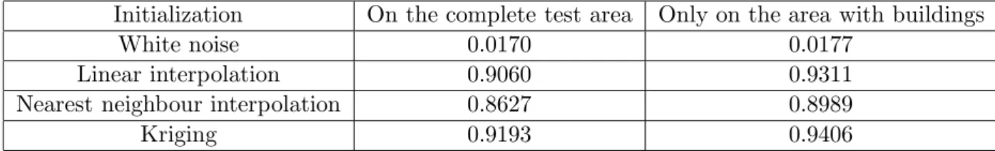
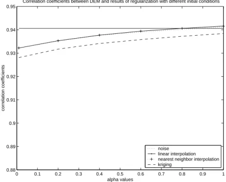
Nous pouvons raisonnablement supposer que les donn´ees laser ont une bonne pr´ecision et n’ont pratiquement pas de bruit. Au contraire, les donn´ees de CMB sont tr`es perturb´ees par le bruit et par les rayonnements. De plus, ces derni`eres sont le r´esultat de la convolution de la carte du ciel avec la r´eponse impulsionnelle du capteur. Les propri´et´es de la surface `a reconstruire ainsi que les techniques d’acquisition doivent donc ˆetre prises en compte. Pour l’interpolation de donn´ees laser, nous con-sid´erons que le probl`eme est mal-pos´e et adaptons une fonction de coˆut pour les donn´ees irr´eguli`erement espac´ees. Les bords des bˆatiments dans des zones urbaines formant de fortes discontinuit´es, nous utilisons des fonctions potentielles qui pr´eservent les discontinuit´es. La minimisation d’une telle fonction de coˆut permet d’obtenir la surface recherch´ee. Les r´esultats de cette approche sont compar´es `a quelques m´ethodes bien connues pour l’interpolation de donn´ees irr´eguli`erement espac´ees, `a savoir l’interpolation lin´eaire, l’interpolation au plus proche voisin et le krigeage. En utilisant la corr´elation et l’erreur absolue moyenne, nous montrons que ces m´ethodes fournissent des r´esultats moins bons que la minimisation d’une fonction de coˆut, qui impose les propri´et´es d´esir´ees `a la surface r´esultante. Quand on les compare visuelle-ment avec l’image de r´ef´erence, les images qui ont une faible erreur absolue moyenne sont plus satisfaisantes que celles avec une bonne corr´elation. Les exp´erimentations sont faites sur deux ensembles de donn´ees r´eelles. Pour chacun d’entre eux, la strat´egie de balayage et la densit´e des points ´etaient diff´erentes.
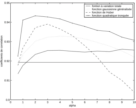
Nous adaptons la fonction de coˆut `a l’interpolation de donn´ees laser. Pour ce faire, nous avons d´efini un voisinage ad´equat. Nous pr´esentons et discutons les r´esultats obtenus avec diff´erentes fonctions potentielles et en faisant varier le coefficient du terme de r´egularisation. Nous ´etudions de mani`ere approfondie l’influence du choix des fonctions potentielles sur les propri´et´es de la surface reconstruite repr´esentant des zones urbaines. Pour choisir la fonction potentielle d’attache aux donn´ees dans la fonction de coˆut, nous utilisons des r´esultats th´eoriques r´ecents. Pour les donn´ees laser, le choix classique de la fonction quadratique pour le terme d’attache aux donn´ees ne m`ene pas `a des r´esultats satisfaisants sur des zones urbaines.
En dehors de l’interpolation au plus proche voisin, de l’interpolation lin´eaire et du krigeage, nous essayons ´egalement la m´ethode de binning et la minimisation de fonction de coˆut pour les mesures simul´ees d’anisotropies du CMB. La surface com-pos´ee par ces mesures est lisse si l’on ne fait pas la d´econvolution. Dans ce cas, la r´egularisation de Tikhonov est appliqu´ee aux donn´ees bruit´ees. Le krigeage n’avait pas ´et´e appliqu´e auparavant pour interpoler des donn´ees du CMB. Nous avons montr´e que cette m´ethode donne de bons r´esultats. Le krigeage sur un voisinage fixe permet l’ex´ecution rapide sur de grands ensembles de donn´ees. C’est donc un avantage pour l’interpolation des donn´ees r´eelles. Cependant, bien que le krigeage surpasse la
min-imisation de fonction de coˆut, celle-ci peut ˆetre adapt´ee `a la fois `a la d´econvolution et `a l’interpolation. Il vaut alors mieux dans ce cas utiliser une fonction quadratique tronqu´ee pour le terme de r´egularisation, afin de reconstruire les sources ponctuelles.
Les conclusions suivantes r´esultent de nos travaux sur les m´ethodes d’interpolation pour des donn´ees irr´eguli`erement espac´ees :
- l’interpolation au plus proche voisin convient quand la densit´e de la grille r´eguli`ere impos´ee est inf´erieure `a la densit´e des donn´ees originelles irr´eguli`erement es-pac´ees. Les donn´ees ne doivent cependant avoir aucun bruit. L’avantage de cette m´ethode est sa vitesse et simplicit´e ;
- l’interpolation lin´eaire bas´ee sur triangle fonctionne bien quand la densit´e des points de grille est inf´erieure ou ´egale `a la densit´e de donn´ees originale ;
- le krigeage est bas´e sur les param`etres de variogramme et n´ecessite leurs estima-tions avant d’employer cette m´ethode. L’´evaluation des param`etres est souvent faite manuellement, mˆeme s’il est possible de la faire automatiquement. A la diff´erence des deux m´ethodes pr´ec´edentes, le krigeage peut supprimer le bruit, dans la mesure o`u le param`etre de p´epite contient dans l’algorithme les informa-tions sur le bruit ;
- le binning, souvent utilis´e en astronomie, fait la moyenne des valeurs des donn´ees `a l’int´erieur de chaque pixel et peut ainsi diminuer le bruit. L’inconv´enient de cette m´ethode est que la densit´e des points des donn´ees doit ˆetre au moins dix fois sup´erieure `a la densit´e de la grille r´eguli`ere pour obtenir de bons r´esultats. Il est ´egalement souhaitable d’avoir des points distribu´es de fa¸con homog`ene ; - l’approche par fonction de coˆut a l’inconv´enient de faire intervenir un coefficient
pour le terme de r´egularisation. Les avantages de la m´ethode sont sa flexibilit´e et sa capacit´e pour interpoler diff´erents types de surfaces en utilisant diff´erentes fonctions potentielles. Des gradients calcul´es sur les donn´ees originales pour-raient ˆetre incorpor´es dans le terme d’attache aux donn´ees.
Grˆace aux exp´erimentations utilisant la minimisation d’une fonction de coˆut pour les donn´ees laser, nous avons mis en ´evidence les r´esultats suivants :
- les valeurs du coefficient du terme de r´egularisation doivent ˆetre sup´erieures ou ´egales `a 1 ou pour obtenir de bons r´esultats ;
- le voisinage d’un pixel de la grille a d’abord ´et´e d´efini comme ´etant l’ensemble des ´echantillons inclus dans le plus petit cercle contenant les huit plus proches pixels voisins du pixel ; les exp´erimentations ont prouv´e qu’un tel voisinage est un bon choix quand :
1) la densit´e des points de la grille r´eguli`ere est approximativement ´egale `a la densit´e des points des donn´ees ;
- quand une des deux conditions, mentionn´ees ci-dessus n’est pas rencontr´ee, nous proposons une autre d´efinition du voisinage qui doit inclure des points des donn´ees dans diff´erentes directions par rapport au pixel. Cette strat´egie est d´efinie suite aux exp´erimentations faites sur les donn´ees laser d’Amiens, o`u les ´echantillons forment les lignes parall`eles tr`es espac´ees ;
- la taille recommand´ee du voisinage doit ˆetre approximativement ´egale `a la dis-tance entre les lignes de balayage. Cette disdis-tance peut ˆetre calcul´ee avant mˆeme l’acquisition de donn´ees, en tenant compte des param`etres techniques du syst`eme de balayage et de la vitesse pr´evue de l’avion ou de l’h´elicopt`ere employ´e.
Plusieurs directions sont envisageables pour am´eliorer les r´esultats sur l’interpolation de donn´ees laser. En ce qui concerne la technique de minimisation d’une fonction de coˆut, les travaux futurs suivants pourront ˆetre envisag´ees. La d´efinition du voisinage peut d’abord ˆetre chang´ee : nous pourrions ainsi choisir les points voisins du pixel selon le diagramme de Voronoi. Le premier avantage de ce choix serait l’anisotropie des donn´ees choisies. Le deuxi`eme avantage serait d’avoir un param`etre en moins : il n’y aurait alors aucun besoin de fixer la taille du voisinage, puisque celui-ci chang-erait automatiquement `a chaque fois selon la proximit´e des ´echantillons. Une autre am´elioration consisterait `a changer de fonction de coˆut pour que le choix des fonc-tions potentielles d´epende de l’´evaluation locale du gradient des ´echantillons. Nous pourrions ´egalement employer diff´erentes fonctions potentielles dans diff´erentes direc-tions `a l’int´erieur d’une clique, en essayant de renforcer les discontinuit´es de la surface. Une forme et une taille diff´erentes des cliques pourraient ˆetre envisag´ees pour tenir compte de quelques propri´et´es g´eom´etriques ´evidentes des zones urbaines, telles que les lignes droites. Ind´ependamment de l’interpolation bas´ee sur la fonction de coˆut, nous pourrions ´etudier des fonctions d’ondelettes pour l’interpolation de la surface avec des discontinuit´es. Une autre possibilit´e reviendrait `a tenir compte de la struc-ture des grilles d’´echantillonnage. Le filtrage it´eratif de m´ediane constitue ´egalement une perspective int´eressante pour de futurs travaux. C’est une technique simple et rapide qui est connue pour avoir les propri´et´es de la diffusion anisotrope. Elle aiderait ainsi `a pr´eserver les discontinuit´es. Enfin, les r´esultats de l’interpolation lin´eaire sur les donn´ees laser pourraient ˆetre am´elior´ees en utilisant la g´eom´etrie stochastique `a la triangulation de Delaunay sur les bords des bˆatiments.
Concernant les donn´ees du CMB, les recherches pourraient porter sur l’adaptation de la fonction de coˆut et sur quelques autres m´ethodes. La fonction de coˆut pourrait ˆetre adapt´ee `a la d´econvolution tout en interpolant les donn´ees. Cette modification pourrait prendre en compte la forme elliptique de la r´eponse, qui est importante pour les mesures r´eelles d’anisotropies du CMB. Les donn´ees du CMB pourraient ˆetre con-sid´er´ees comme somme de la surface lisse, repr´esentant les anisotropies du CMB, et de la surface compos´ee des sources ponctuelles. Les diff´erentes contraintes, impos´ees `a chacune des deux surfaces, pourraient ainsi am´eliorer les r´esultats. Plusieurs m´ethodes de reconstruction pour les signaux `a bande limit´ee pourraient enfin ˆetre appliqu´ees aux donn´ees du CMB. Cependant, dans ce cas, le signal devrait ˆetre ´echantillonn´e selon le crit`ere de Nyquist `a la moyenne.
Le but des exp´erimentations avec interpolation de donn´ees du CMB est d’obtenir une m´ethode qui fonctionne pour des coordonn´ees sph´eriques. Les donn´ees r´eelles du CMB sont en effet en coordonn´ees sph´eriques. Or, les m´ethodes pr´esent´ees dans la th`ese utilisent des voisinages locaux qui peuvent ˆetre consid´er´es comme localement plans.
En conclusion, cette th`ese nous aura permis de reposer le probl`eme de l’´echantillonnage sur des donn´ees irr´eguli`erement espac´ees et de montrer que celui-ci constituait un probl`eme inverse mal pos´e. Nous avons ´egalement pu d´efinir des mod`eles math´ematiques adapt´es aux donn´ees originales afin d’obtenir des r´esultats concluants. De plus, en analysant ceux-ci, nous avons pu proposer de nombreux perspectives visant `a les am´eliorer.
Contents
Introduction 13
1 Sampling theory 16
1.1 Introduction . . . 16
1.2 Uniform sampling . . . 16
1.2.1 Shannon sampling theory . . . 16
1.2.2 Papoulis generalization of the sampling theorem . . . 19
1.2.3 Extension of Papoulis theorem for non-bandlimited signals . . . 21
1.2.4 Sources of errors . . . 22
1.3 Classification of sampling sets . . . 23
1.3.1 One-dimensional sampling sets . . . 23
1.3.2 Two-dimensional sampling sets . . . 24
1.3.3 Hexagonal sampling . . . 28
1.4 Nonuniform sampling . . . 30
1.4.1 Nonuniform sampling for bandlimited signals . . . 31
1.4.2 Nonuniform sampling for non-bandlimited signals . . . 32
1.4.3 Jittered sampling . . . 33
1.4.4 Wavelets on irregular grids . . . 35
1.5 Conclusion . . . 36
2 Airborne laser scanning 38 2.1 Introduction . . . 38
2.2 Acquisition technique . . . 38
2.3 Laser data accuracy and properties . . . 44
2.3.1 Comparison with photogrammetry . . . 46
2.4 Applications of laser data . . . 48
2.5 Conclusion . . . 49
3 Interpolation for airborne laser data of urban areas 51 3.1 Introduction . . . 51
3.2 General approaches . . . 52
3.3 Nearest neighbor interpolation . . . 53
3.4 Triangle-based linear interpolation . . . 58
3.5 Kriging . . . 61
3.6 Energy minimization approach . . . 66
3.6.1 Definition of neighborhood . . . 68
3.6.2 Expression for the cost function . . . 70
3.6.3 Potential functions . . . 71
3.6.4 Optimization algorithm . . . 74
3.6.5 Example on the synthetic model . . . 75
3.7 Conclusion . . . 76
4 Experimental results on laser data 78 4.1 Introduction . . . 78
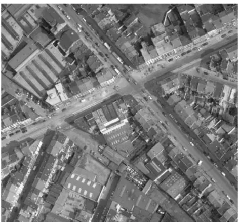
4.2 Data of Brussels . . . 78
4.2.1 Data description . . . 78
4.2.2 Nearest neighbor interpolation . . . 81
4.2.3 Linear interpolation . . . 83
4.2.4 Kriging . . . 83
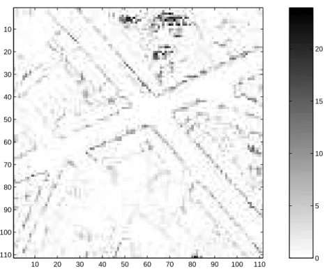
4.2.5 Comparison of results . . . 85
4.2.6 Energy minimization method . . . 90
4.3 Data of Amiens . . . 100
4.3.1 Data and ground truth description . . . 100
4.3.2 Classical interpolation approaches . . . 103
4.3.3 Energy minimization method and comparison of results . . . 106
4.4 Conclusion . . . 112
5 Cosmic microwave background 115 5.1 Introduction . . . 115
5.2 CMB radiation . . . 115
5.3 Archeops experiment . . . 118
5.4 Planck mission . . . 119
5.5 Data description . . . 121
6 Experiments on simulated CMB data 125 6.1 Introduction . . . 125
6.2 Interpolation methods . . . 125
6.2.1 Nearest neighbor interpolation . . . 126
6.2.3 Kriging . . . 135
6.2.4 Binning . . . 143
6.3 Comparisons with the reference . . . 145
6.4 Energy minimization . . . 150
6.5 Kriging versus binning: performance analysis . . . 152
6.6 Conclusion . . . 160
Introduction
Interpolation problems have been widely considered in many areas of applied science, and one of them is signal and image processing. Development of digital technologies leads to the measurement techniques that provide discretized values of the signals one wants to acquire. These measurements may be obtained at odd positions and not on regular grids as expected. In this framework it is very important to have interpolation methods that correspond to the physics of the signal to measure. In other words, an a-priori model of the signal is often useful for its interpolation.
Nowadays a lot of methods allow different types of image processing. Most of these methods have been well studied both in theory and practice. But very often they can only be applied to the data on a regular grid. In the same time, some acquisition techniques are able to get the measurements either on a jittered or on an irregular grid. This is the case for many airborne or spaceborne remote sensing techniques. Even though sometimes the sampling is performed on the regular grid in the reference system of the sensor, the resulting georeferenced points are scattered. Therefore interpolation and resampling of the original data will produce the data on the regular grid and will enable us to perform further processing and analysis: visualization, segmentation, fusion, etc.
The wide range of the interpolation techniques, available at the present time, gets smaller when one wants to interpolate the values that are initially distributed on an irregular grid. It is the topic that we consider in the thesis. Moreover, interpolating a signal that is non-bandlimited and whose measurements are scattered in space is not a trivial problem and requires some studies to be done. This problem is considered in the thesis while working with airborne laser scanning data. The data has been acquired over the urban areas. Since the urban areas often consist of streets and buildings, the edges of the buildings form discontinuities and so the signal to interpolate is non-bandlimited.
Obtaining 3D city models is important for several reasons. They include creation and updating of Geographical Information Systems for towns, urban planning and development projects that are supposed to prevent distribution of polluting substances, or provide transport network planning, telecommunication antennas placements. 3D cities in virtual reality are also one of the possible applications of remote sensing on urban areas. Airborne laser scanning is a fast and precise data acquisition technique that has been tested over urban areas. This technique itself is still a subject of research and development. We present a review on the laser scanning acquisition technique since it leads to the understanding of the nature of the acquired data, for example the noise
and the precision of the measurements. Such parameters are helpful for developing the suitable interpolation method.
The second part of the thesis is devoted to cosmic microwave background (CMB) data interpolation. This kind of data is also on an irregular grid. The surface to interpolate is considered to be smooth as long as no deconvolution is made. Acquiring and treating the cosmic microwave background data has been an area of great scientific interest during the last decades. It is a topic of cosmology - the science about the origin of our Universe. There are models of the Universe, developed by astronomers, and it is considered that some parameters may determine the age, the shape and the matter of the Universe. However, these parameters are to be calculated from the maps of CMB. These maps must be on a regular grid, while the original measurements are not. So the problem of irregularly spaced data interpolation should be considered in this case. The manuscript is organized in the following way. In Chapter 1 the theoretical aspects of sampling are considered. Though we are interested in the irregular sampling theories, we start this chapter by the well known theorem of Shannon, because it served as a starting point for most of the later research in sampling. We realize that among problems of irregular sampling there is a problem of the optimal grid size. It could be a subject of research of the thesis. Several approaches could be tried in this direction: information density measures, degrees of freedom or minimum of the entropy approach. In this chapter we pay attention to the theory of non-uniform and random sampling which is the case of the data we have. We consider a classification of sampling sets in one and in two dimensions. Random sampling of non-bandlimited signals is the area of interest in the current research in applied and pure mathematics.
In Chapter 2 we consider the laser scanning technique, its precision and properties, as well as the range of parameters for the existing laser scanning systems and practical applications of such kind of data. In the interpolation methods presented and imple-mented in the following chapters we would like to take into account not only the form and properties of the scanned surface, but also the acquisition technique. That is why many technical details are given in this chapter. For example, it would be interesting to simulate the airborne laser scanning acquisition. In this case the analysis of the sources of noise must be done. As we will see in this chapter, the performance of laser scanning is still a subject of research, especially when it concerns urban areas. In this chapter we also name the applications of the airborne laser scanning which ex-plain why this technique has received so much attention of the remote sensing research community in recent years.
Chapter 3 describes the general approaches for scattered data interpolation and also contains the description of the methods to be used in experiments with the real data. The first two described methods are nearest neighbor and triangle based linear interpolation. These methods are fast and simple and we would like to know what results they give in order to be able to introduce a better approach more suited for our data. The third described method is kriging. It is developed in geostatistics for irregularly spaced data interpolation. The assumptions used by this method are valid for the cosmic microwave background anisotropies. Nevertheless, we will present the results of this method on airborne laser scanning data too. The problem of scattered
data interpolation can be regarded as an ill-posed inverse problem. Therefore we present an energy minimization method and we adapt it to laser scanning data. We will use the potential functions that are known for their edge preserving properties. We present the definition of the neighborhood for our problem, expression of the cost function as well as the choice of the optimization algorithm.
These methods are implemented and their results are presented in Chapter 4. We apply the methods to two real data sets. It will help us to evaluate the interpolation methods, because the two sets are acquired by different laser scanning systems and therefore have different properties: sampling patterns are very different. We compare the results with the reference and make conclusions about their performance.
In Chapter 5 there is a short introduction to the CMB theory as well as to the CMB data acquisition technique. The described technique will be used in 2007 by the European Space Agency when it launches the Planck satellite. This mission will provide the most precise and complete data ever acquired on the CMB.
Chapter 6 presents some results and their comparison over the simulated CMB data. The simulated data respects the sampling pattern as it is supposed to be for the Planck mission. We apply the interpolation methods presented above to this kind of the data and we also implement binning - an averaging technique, often used in astronomy. The main difference between the CMB anisotropies data and the laser data is not only in the type of the surface that is scanned but also in the fact of having very strong noise in the CMB anisotropies measurements. We simulate it as white noise and we study the performance of the methods on the noisy data.
The chapter of conclusions presents the summary and proposes some directions for the future work.
Chapter 1
Sampling theory
1.1
Introduction
This chapter presents some theoretical aspects of the sampling theory. This theory has received a lot of attention in the several recent decades. Especially is important if we take into account the fast development of digital technologies. When real world signals are acquired through digital devices, they are often sampled on the regular grids with equal distances between nodes. For images, the most widely used grid are square grids, though there are some cases when hexagonal ones are preferred. The theory of sampling is supposed to answer many questions on the optimal acquisition of data and its reconstruction and further processing afterwards. In this framework signals may be divided on bandlimited and non-bandlimited ones, and grids are divided on uniform and nonuniform.
The chapter contains three sections. In the first section we consider uniform sam-pling and the theorems of Shannon and Papoulis. These theorems are now considered as classical ones, and we present them in the text, because most of the later research and development of the sampling theory relies on them. The second section contains a classification of sampling sets from the theoretical point of view. It shows the possible variety of sampling sets, some of which are already applied in technology and allow reconstruction and resampling. It should be emphasized that after the regular square grids, one can consider hexagonal grids as quite well studied and applied ones. In the third section we consider nonuniform grids. Taken into account the classification made in the previous section, we notice, that most of the theories are developed either for jittered or for irregular sampling.
1.2
Uniform sampling
1.2.1
Shannon sampling theory
The basics of the sampling theory was developed in the beginning of the last century. It is often associated with names of Nyquist, Whittaker, Kotel’nikov and Shannon
[Jerri, 1977]. The sampling theorem given by Shannon is the following [Shannon, 1949]. If a function f (t) contains no frequencies higher than W cps, it is completely deter-mined by giving its ordinates at series of points spaced 1/2W seconds apart. The rate 1/2W is called Nyquist rate. Let xn be the nth sample, then the function f (t) is
represented by f (t) = ∞ X n=−∞ xn sinπ(2W t − n) π(2W t − n) .
Emphasizing that only stable sampling is meaningful in practice, Landau proved that it cannot be performed at a lower rate than the Nyquist rate [Jerri, 1977]. Considering the Shannon sampling theorem and using the Parseval equation, Landau gave an in-terpretation that relates the Nyquist rate with the stability of the sampling expansion.
1) Every signal f (t) of finite energy, i.e. R∞
−∞f2(t)dt < ∞, and bandwidth W
may be completely recovered in a simple way, from the knowledge of its samples taken at the Nyquist rate of 2W per second. The recovery is stable in the sense of Hadamard, such that a small error in sample values produces only a correspondingly small error in the recovered signal.
2) Every square-summable sequence of numbers may be transmitted at the rate of 2W per second over an ideal channel of bandwidth W by being represented as the samples of an easily constructed band-limited signal of finite energy.
In relation to the required Nyquist rate for the transmitted sequence of samples or the recovered ones, Landau considered other configurations, besides the band-limited finite energy signals, in order to improve such rates. He proved the following two results.
1) Stable sampling cannot be performed at a lower rate than the Nyquist rate. 2) Data cannot be transmitted as samples at a rate higher than the Nyquist rate
regardless of the location of sampling instants, the nature of the set of frequencies which the signal occupy, or the method of construction.
These results also apply to bounded signals besides finite energy signals. For the multidimensional sampling theorem [Marks, 1991] let’s consider
- x(~t) as a multidimensional bandlimited function;
- X(~u) as its spectrum; the function x(~t) is defined to be bandlimited if X(~u) = 0 outside of an N-dimensional sphere of finite radius;
- S(~u) as the replication of |detP |X(~u) as a result of sampling, where the period-icity matrix P must be chosen so that the spectral replications do not overlap and therefore alias.
The multidimensional sampling theorem can be summarized in the following way: x(~t) =X ~ m x(Q ~m)fc(~t − Q ~m), where fc(~t) = |detQ| Z ~ u∈Cexp(j2π~u T~t)d~u,
C is a periodicity cell for the spectrum, the Q matrix it the sampling matrix and it dictates the geometry of the uniform sampling. The sampling density (samples/unit area) corresponding to Q is
SD = 1
|detQ| = |detP |.
The Nyquist rate can be generalized to higher dimensions. In this case it is called Nyquist density - the density resulting from maximally packed unaliased replication of the signal’s spectrum. For the case of two dimensions the Nyquist density corresponds to the hexagonal sampling geometry.
There have been a number of significant generalizations of the sampling theorem [Marks, 1991, Jerri, 1977]. Some are straightforward variations on the fundamental cardinal series. Oversampling, for example, results in dependent samples and allows much greater flexibility in the choice of interpolation functions. It can also result in better performance in the presence of sample data noise. Kramer generalized the sampling theorem to signals that were bandlimited in other than the Fourier sense.
Bandlimited signal restoration from samples of various filtered versions of the signal is the topic addressed in Papoulis’ generalization of the sampling theorem [Papoulis, 1977]. Included as special cases are recurrent nonuniform sampling and simultaneously sampling a signal and one or more of its derivatives.
New generalizations of the sampling theorem are still being developed [Unser, 2000, Vaidyanathan, 2001].
For example, in [Unser, 1994] the theoretical framework for a general sampling theory is given. The theory restates the theorem of Shannon. The main goal of the general sampling theory presented in the paper is to adapt the process of signal reconstruction to non-ideal acquisition devices. The matter is that on the theorem of Shannon the signal is considered to be sampled by Dirac functions, while on practice one has to deal with an impulse response of a sensor. The convolution with this impulse response function is performed before the signal is sampled. The paper proposes a reconstruction and a correction filters in order to reconstruct the signal. The signal may not be bandlimited. Lifting the condition of a bandlimited signal leads to the approximation of it. It is proved that in theory one can reconstruct a signal, sampled by non-ideal acquisition devices, and this reconstruction will be consistent. It means that if we reinject the reconstructed signal into the acquisition device, then the samples will be the same as the ones of the signal reconstructed previously. The presented theory
is developed only for 1D case, though it is supposed that it can be extended to more dimensions. Another remark concerns the fact that noise is not taken into account, and more development should be done to adapt the presented theory for a noise.
1.2.2
Papoulis generalization of the sampling theorem
There are a number of ways to generalize the manner in which data can be ex-tracted from a signal and still maintain sufficient information to reconstruct the signal [Marks, 1991]. Shannon noted that one could sample at half the Nyquist rate without information loss of it, at each sample location, two sample values were taken: one of the signal and one of the signal’s derivative. The details were later worked out by Linden who generalized the result to restoring from a signal sample and samples of its first N − 1 derivatives taken every N Nyquist intervals. It is also possible to choose any N distinct points within N Nyquist intervals. If signal samples are taken at these locations every N Nyquist intervals, it is the question of restoration from interlaced (or bunched) samples.
All of these cases are subsumed in a generalization of the sampling theorem de-veloped by Papoulis (1977). The generalization concerns restoration of a signal given data sampled at 1/Nth the Nyquist rate from the output of N filters into which the
signal has been fed.
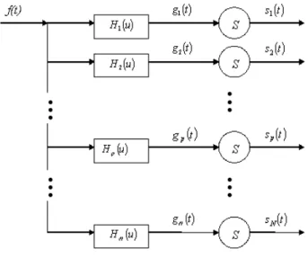
Let {Hp(u)|p = 1, 2, ..., N} be a set of N given filter frequency responses and let
f (t) have bandwidth B. As shown in Figure 1.1, f (t) is fed into each filter.
Figure 1.1: Generation of sample data from Papoulis’ generalized sampling theorem. The encircled S is a sampler.
The outputs are
Each output is sampled at 1/Nth the Nyquist rate. The signal of samples obtained
from the pth filter are
sp(t) = ∞ X n=−∞
gp(nTN)δ(t − nTN),
where TN = 1/2BN and BN = B/N. The problem is to restore f (t) from this set of
functions or, equivalently, the sample set
gp(nTN|1 ≤ p ≤ N, −∞ < n < ∞).
According to Papoulis’ theorem, f (t) = N X p=1 ∞ X n=−∞ gp(nTN)kp(t − nTN) where kp(t) = Z B B−2BN
Kp(u; t)ej2πutdu
and the Kp(u; t)’s are the solutions of the simultaneous set of equations
2BN N X p=1
Kp(u; t)Hp(u − 2mBN) = exp(−j2πmt/TN)
over the parameter set 0 ≤ m ≤ N, B − BN < u < B and −∞ < t < ∞. If N = 1
and H1(u) = 1, then the Shannon sampling theorem results.
The theorem of Papoulis can be used for signal interpolation after recurrent nonuni-form sampling. Let αp|p = 1, 2, ..., N denote N distinct locations in N Nyquist
inter-vals (Figure 1.2).
Figure 1.2: Illustration of Nthorder recurrent nonuniform sampling. In each N Nyquist
intervals, samples are taken at these same relative locations.
A signal is sampled at these points every N Nyquist intervals. Thus there is knowledge of the data
{f (αp+
m 2BN
Such sampling is also referred as interlaced (or bunched) sampling. The generalized sampling theorem is applicable here if the filters are
Hp(u) = exp(j2παpu); 1 ≤ p ≤ N.
On the interval (0, TN) the resulting interpolation functions are:
kp(t) = sinc[2BN(t − αp)] N Y q=1; q6=p sin[2πBN(t − αq)] sin[2πBN(αp− αq)] .
By utilizing the Papoulis’ generalized sampling expansion, it was demonstrated [Cheung, 1993] that there is a class of sampling theorems which are ill-posed. In particular, given the samples are contaminated with noise, the interpolation noise variance is unbounded for these ill-posed sampling theorems.
The multidimensional extension of Papoulis’ theorem is utilized to reduce the sam-pling density of multidimensional band-limited functions. The reduction leads to the minimum sampling density, which is equal to the area of the support of the function’s Fourier spectrum.
For the data we want to interpolate on this thesis, there are two limitations for using the theorem of Papoulis. At first, the signal to interpolate is non-bandlimited. It is true when we consider the airborne laser data over urban areas, which we will describe in the following chapter. At second, the sampling strategy in the real data cannot be modeled as recurrent nonuniform sampling. Especially it is valid for the areas where the scanning strips overlap. The cosmic microwave background anisotropies also can be described as non-bandlimited signals when we consider the point sources.
The theory of Papoulis has been extended for the case of non-bandlimited signals, but in this case it is possible to obtain an approximation of a signal instead of a reconstruction [Unser et al., 1998].
1.2.3
Extension of Papoulis theorem for non-bandlimited
sig-nals
In this section we describe the work of Unser and Zerubia on the generalized sampling theory [Unser et al., 1998]. The main point of the theorem of Papoulis is that there are many possible ways of extracting data from a signal for a complete characterization. The standard approach of taking uniform signal samples at the Nyquist rate is just one possibility among many others. Typical instances of generalized sampling that have been studied in the literature are interlaced and derivative sampling. Later, an interest has been strengthen in such alternative sampling schemes for improving image acquisition. For example, in high resolution electron microscopy there is an inherent tradeoff between contrast and resolution. It is possible, however, to compensate for these effects by combining multiple images acquired with various degrees of defocus-ing. Super-resolution is another promising application where a series of low resolution images that are shifted with respect to each other are used to reconstruct a higher resolution picture of a scene.
Papoulis’ generalized sampling theory provides an attractive framework for ad-dressing most restoration problems involving multiple sensors or interlaced sampling. However, the underlying assumption of a bandlimited input function f (x) is very re-strictive. It is because most of the real world analog signals are time or space limited which is in contradiction with the bandlimited hypothesis. Another potential difficulty is that Papoulis did not explicitly translate his theoretical results into a practical nu-merical reconstruction algorithm.
The main contributions of the work of Unser and Zerubia are as follows. First, they propose a much less constrained formulation where the analog input signal can be almost arbitrary, typically in the space of finite energy functions (Figure 1.3). This
Figure 1.3: Generalized sampling procedure [Unser et al., 1998]. The left part of the block diagram represents the measurement process which is performed by sampling the output of an m channel analysis filterbank. The sampling operation is modeled by a multiplication with a sequence of dirac impulses. The right part describes the reconstruction process which involves the synthesis functions. The system produces an output function that is a consistent approximation of the input signal f (x). is only possible because the Papoulis and Shannon’s principles of a perfect recon-struction are replaced by the weaker requirement of a consistent approximation. That means that the reconstructed signal provides exactly the same measurements as the input signal if it was reinjected into the system. The second contribution is the con-sideration of a more general form of the reconstruction subspace. In this way the results are applicable for non-bandlimited signal representation models. At third, the implementation issue is addressed explicitly and a practical reconstruction algorithm is proposed, though the results on the signals with discontinuities are not presented.
1.2.4
Sources of errors
Various errors may arise in the practical implementation of the sampling theorems [Jerri, 1977, Jerri, 1993, Feichtinger et al., 1993]. This includes the truncation error which results when only a finite number of samples are used instead of the infinite
samples needed for the sampling representation, the aliasing error which is caused by violating the band-limitedness of the signal, the jitter error which is caused by sampling instants different from the sampling points, the round-off error, and the amplitude error which is the result of the uncertainty in measuring the amplitude of the sample values.
For the band-limited signal
f (t) =
Z a
−aF (u)e
iutdu
and its sampling representation f (t) = ∞ X n=−∞ f (nπ a ) sin(at − nπ) (at − nπ)
the truncation error ǫT is the result of considering the partial sum fN(t) with only
2N + 1 terms of the infinite series, ǫT = f (t) − fN(t) = X |n|>N f (nπ a ) sin(at − nπ) (at − nπ) .
In practice, the signals are not necessarily band-limited in the sense required by the Shannon sampling expansion. The aliasing error ǫA(t) = f (t) − fs(t) is the result
from applying the sampling theorem representation fs(t) to signals f (t) with samples
f (nπ/a) even when they are not band-limited or band-limited to different limits than those used in sampling expansion.
The amplitude error is caused by the uncertainty in the sample values due to either quantization or to some fluctuation where the round-off error may be considered as a special case.
The jitter error results from sampling at instants tn = nT + γn which differ in a
random fashion by γn from the required Nyquist sampling instants nT .
1.3
Classification of sampling sets
1.3.1
One-dimensional sampling sets
For one-dimensional sampling sets the possibilities for creating different types of sets are not as large as they are in two dimensions. The following description of sampling geometries is sorted by the different steps of irregularity [Schmidt, 1997].
The geometry of the regular sampling sets depends on the length of the signal. If n is the length of the vector and k is the amount of sampling points (k is a divisor of n), then the difference between the regular sampling structures is determined only by the density k/n of the sampling points.
The periodic sampling sets are a more general way of creating geometries in the one-dimensional case. No strict regular periodicity is demanded, a sampling set may
be composed of some shifted subsets of it. Then the resulting set is periodic in the way that the shifted subsets are repeated periodically. So such a periodic sampling set is not regular, but has some properties left. In the two-dimensional case this form of sampling is called bunched sampling. The two-dimensional periodicity gives more information about the sampling set, than in irregular sampling, and can be used to improve the reconstruction.
Irregular (random) sampling sets mean just making a random sampling. There are different parameters which can be varied (as the density of the sampling set), but the structure of irregularity is granted.
1.3.2
Two-dimensional sampling sets
In the two-dimensional case the variability of different sampling sets is increasing rapidly in comparison with the one-dimensional case, because there are not only the product sampling sets of the corresponding one-dimensional possibilities, but also some new variations which do not have an equivalent in the 1-D problem (for example, spiral sampling). The following two-dimensional sampling sets are arranged by increasing irregularity and at the same time by increasing the number of possible sampling sets depending on the sampling method [Schmidt, 1997].
A square (or regular) sampling set in two dimensions (Figure 1.4) can be treated like a multiplication of two one-dimensional sampling sets. The square sets can be described in matrix form by multiplying two regular one-dimensional sets a, a′, which
have the same coordinates and where ′ denotes the transpose: C = a′ ∗ a.
Figure 1.4: A square sampling set (regular geometry).
A rectangular sampling set (Figure 1.5) differs from a square set, because the multiplication is not done by two similar regular vectors but it is performed by two different regular vectors.
Figure 1.5: A rectangular sampling set.
As the result the grid has two different step widths. The rectangular sets are more general than the square sets.
The double periodic sampling sets (Figure 1.6) are created through multiplication of two one-dimensional periodic vectors.
Figure 1.6: A periodic sampling set.
They are a special type of the product sampling sets because they need to be periodic in both directions.
Product sampling sets are the easiest way of getting a two-dimensional sampling geometry because they can be generated by just multiplying two arbitrary vectors. An
example of image reconstruction from product sampling set is given in [Feichtinger et al., 1994]. Superposition of three different product sampling sets is used for RGB color coding
for some cameras. The grid received by this method is called Bayer mask.
Bunched sampling sets (Figure 1.7) can be obtained by first taking a sparse matrix with regular or periodic entries and then defining some shift vectors with components in both directions to define an overlay of two or more of these matrices.
Figure 1.7: A bunched sampling set.
The bunched set can also be described as a form of irregular sampling because it is possible to look on it as a simple product set with missing points inside. But this description is less useful because of the loss of information about the structure of the set and way of generating it. Hexagonal sampling sets and octagonal sampling sets are examples of bunched sets.
Elliptic, polar or spiral sampling sets (Figure 1.8) occur in astronomical obser-vations. When the astrophysical data acquisition is performed with the equipment installed on Earth, spiral sampling sets will be caused by the movement of the Earth. Polar sampling is used both in biomedical imaging (computer tomography) and in remote sensing (radar data).
There are interpolation methods developed for this kind of sampling sets [Stark, 1993]. Quasiregular sampling sets are generated by thinning out or filling in some amount of points (i.e. 10 percent) from a regular hexagonal, octagonal or product sampling set. Normally, a structure of a quasiregular sampling set is still visible for a human eye. Quasiregularity also means that regularly distributed sampling points may be distorted from their original position by a small amount. That is also not a regular set, but the irregularity is not too large.
Irregular sampling sets (Figure 1.9) have no internal structure to exploit and so all algorithms have to be kept generally.
In general, the classification of sampling sets, presented in this section, is mostly of a theoretical interest, because most of the real sampling sets have either jittered regular structure (like images taken in some remote sensing applications) or they are irregular, random. Considering the sampling pattern of airborne laser scanning,
pre-Figure 1.8: A linear expanding spiral sampling set.
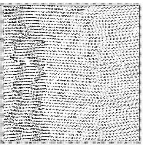
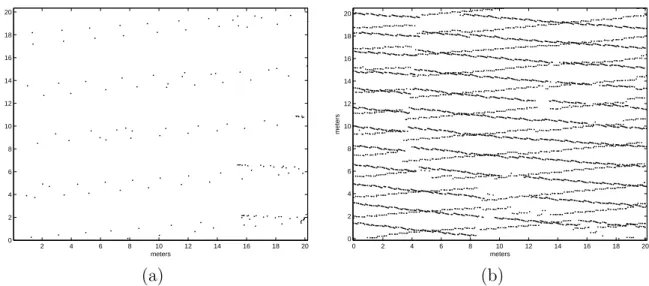
sented later in this thesis, we can say that the sampling set strongly depends on the scanning system. Airborne laser scanning in theory can be represented by a sampling set composed of circles, or by jittered hexagonal grid, or by a particular periodic set. But in practice scan lines overlap and then it is difficult to find a structure in the obtained data (Figure 1.10, 1.11). Recently it has been clear that for urban areas it
Figure 1.10: An irregular grid produceed by laser scanning over an area of 200 × 200 meters.
is necessary that large parts of scan lines overlap, because it will provide more dense data and therefore more information on the area to scan, especially on the edges of buildings.
1.3.3
Hexagonal sampling
The hexagonal sampling (Figure 1.12) offers substantial savings in machine storage and arithmetic computations [Schmidt, 1997]. There exist some methods for processing 2D signals sampled on 2D hexagonal arrays. The rectangular sampling set can be treated as a special case of the general non-orthogonal sampling strategy. Especially for bandlimited signals over a circular region of the Fourier plane the hexagonal setting seems to be fruitful and optimal since it reduces the necessary sampling density to the amount of almost 13%. This might lead to a very efficient implementation since this percentage might be won at each iteration of applied iterative algorithms.
5.1271 5.1272 5.1273 5.1274 5.1275 5.1276 5.1277 x 10⁵ 5.4024 5.4024 5.4024 5.4024 5.4024 5.4024 5.4024 5.4024 x 10⁶
Figure 1.11: A sampling pattern of a real laser data: a gap in the data appears because two neighboring stips don’t overlap.
A review of hexagonal sampling is given in [Almansa, 2002]. The motivation of this study was the development of imaging systems, that would use hexagonal sam-pling grids, at the French Space Agency (CNES). In the conclusions of this review, two reasons are given that prevent the extensive use of hexagonal grids and algo-rithms: the fact that display, acquisition and processing hardware is most often better suited for square grids; and the increased complexity of the algorithms under certain circumstances.
1.4
Nonuniform sampling
There are some cases where there is no choice but to process nonuniform data. Some of the examples are:
- data measured in a moving vehicle with fluctuations in speed for applications in remote sensing, where random or uniform samples with jitter are often inevitable; - data tracked in digital flight control;
- data read from and recorded on a tape or disk with speed fluctuations; - data loss due to channel erasures and additive noise.
Interpolation techniques are developed to reconstruct the signal from nonuniform sam-ples.
Unlike uniform sampling, there is no guarantee of the uniqueness of a band-limited signal reconstructed from arbitrary nonuniform samples [Marvasti, 1993]. This is true even when the average sampling rate is equal to the Nyquist rate. For example, let’s suppose there is one solution to a set of nonuniform samples at instances {tn},
and assume that it is possible to interpolate a band-limited function of the same bandwidth at the zero-crossings {tn}. Now, if one adds this interpolated function to
the first solution, one will get another band-limited function (of the same bandwidth) having the same nonuniform samples. Thus, nonuniform samples do not specify a unique band-limited signal. For a given bandwidth, this ambiguity is related to the set {tn}. Therefore, the {tn} instances must be chosen such that the existence of a
unique solution is guaranteed. A set of these sampling instances that assures unique reconstruction is called a sampling set.
The following lemma has been derived: if the nonuniform sample locations {tn}
satisfy the Nyquist rate on the average, they uniquely represent a band-limited signal if the sample locations are not the zero-crossings of a band-limited signal of the same bandwidth. This lemma implies the following corollary: if the average sampling rate of a set of sample locations {tn} is higher than the Nyquist rate, the samples uniquely
specify the signal and {tn} is a sampling set.
In general, the requirements [Feichtinger et al., 1992] for the reconstruction meth-ods for irregularly sampled band-limited functions are:
- constructivity, i.e. a possibly iterative algorithm should allow numerical recon-struction;
- multidimensionality, so that it can be used in signal and image processing or for the interpolation of sequences of images;
- locality, so that the value of a band-limited function at a point is essentially determined by the adjacent sampling values, and more distant sampling values have no influence;
- stability, so that small perturbations of the parameters cause only small errors in the reconstruction.
1.4.1
Nonuniform sampling for bandlimited signals
The main question here is to recover a signal with a limited band-width and known spectral support from irregularly spaced sampling values. The irregular sampling problem for bandlimited 1D and 2D signals has found much interest during the last decade. Most of the results concern 1D case, though. For the case of irregular sampling values no simple formula for reconstruction, such as the one given by Shannon in the case of regular samples, can be expected. Nevertheless, it is still possible to recover a bandlimited irregularly sampled signal completely, if the sampling set is not too sparse.
There are various techniques to reconstruct signals [Strohmer, 1991], such as iter-ative algorithms, the frame method, direct methods (based on the solution of linear
equations using pseudoinverse matrices) and others [Cenker et al., 1991, Feichtinger et al., 1995]. Iterative algorithms received a lot of attention recently [Almansa, 2002], and we will
describe their idea.
Iterative algorithms use the irregularly spaced sampling information about the signal f and the information about the spectral support of f . Iterative two-step algorithms are typical for most of the methods. They are based on a recursion of the form:
fr+1 = PB(Afr),
where A is some approximation operator using only the original irregularly spaced sampling values, and PB is mapping a given signal onto the space of bandlimited
signals with spectrum B. One may think of this mapping as of a smoothing operation, which eliminates the discontinuity of Af . This projection P can be described as a low-pass filter or as a convolution using a sinc-type kernel with the spectrum defined over the set B.
There are several choices available for the approximation operator A [Strohmer, 1991, Feichtinger et al., 1991]. The Wiley-Marvasti method uses just the sampled signal multiplied by a global relaxation factor. The Sauer-Allebach algorithm takes classical interpolation methods in order to obtain the first approximation. Among these meth-ods are: Voronoi method, Sample and Hold method, piecewise linear interpolation,
spline interpolation. The Voronoi method can also be called nearest neighbor inter-polation. In higher dimensions the corresponding construction makes use of Voronoi regions, that is a step function is used, which is constant in the nearest neighborhood of the sampling points. The Sample and Hold method requires twice the Nyquist rate for a complete reconstruction [Strohmer, 1991]. For large gaps this method for con-structing an approximation of the signal is divergent. Piecewise linear interpolation is suitable only when the gaps between samples are not much larger than the Nyquist rate [Strohmer, 1991]. Spline interpolation gives a good approximation of the signal but requires much more computational expenses comparing with the linear interpolation. The adaptive weights method is a more flexible version of the Wiley-Marvasti method and it derives different appropriate weights from the sampling geometry. In 1D case the distances between subsequent points are considered [Feichtinger et al., 1991].
1.4.2
Nonuniform sampling for non-bandlimited signals
There is a class of non-band-limited signals that can be represented uniquely by a set of nonuniform samples. If a band-limited signal goes through a monotonic non-linear distortion, y(t) = f [x(t)], then, although y(t) is a non-band-limited signal, it can be represented by nonuniform samples if tn is a sampling set for the band-limited signal
x(t) [Marvasti, 1993]. The reconstruction scheme is shown in Figure 1.13.
Figure 1.13: Reconstruction of a non-bandlimited signal from nonuniform samples. Necessary and sufficient conditions for such non-band-limited signals have been established [Marvasti and Jain, 1986]. If a band-limited y(t) is transformed into a non-band-limited x(t) through an unknown analytic and monotonic nonlinear operation f (•), then y(t) can be recovered from x(t) within a constant factor, provided that one of the following conditions is satisfied:
1) dy(t)/dt has only real zeros (zero crossings), but f (•) is only analytic and monotonic;
2) dy(t)/dt may have any kind of zeros, but f (•) has the additional condition that df /dy is also monotonic.
Another example is a set of non-band-limited signals generated by a time varying filter when the input is a band-limited signal. If the system has an inverse, then the samples of the output (the non-band-limited signal) are sufficient to reconstruct the signal. This non-band-limited signal is essentially a time-warped version of the band-limited signal.
The results presented above in this section have not been extended for 2D signals and stay to be a purely theoretical setting for the 1D case, because no practical ap-plication was developed. It makes the use of these results impossible for the real data sets treated in this thesis, because the sampling sets we have are in two dimensions and demand a practically applicable algorithm.
1.4.3
Jittered sampling
Jittered samples are nonuniform samples that are clustered around uniform samples either deterministically or randomly with a given probability distribution. This ran-dom jitter is due to uncertainty of sampling at the transmitter end. For deterministic jitter, Papoulis has proposed a method for the recovery. The problem is recovery of x(t) from the jittered samples, x(nT − µn), where µn is a known deviation from nT .
The main idea is to transform x(t) into another function g(τ ) such that the nonuniform samples at tn= nT − µn are mapped into uniform samples τ = nT (Figure 1.14).
Consequently, g(τ ) can be reconstructed from g(nT ) if g(τ ) is band-limited (W ≤
1
2T). x(t) can be found from g(τ ) if the transformation is one-to-one [Marvasti, 1993].
Let’s take the one-to-one transformation as t = τ − θ(τ ), where θ(τ ) is a band-limited function defined as θ(τ ) = ∞ X n=−∞ µnsinc[πW2(τ − nT )],
where W2 ≤ 2T1 is the bandwidth of θ(τ ). Since the transformation is one-to-one, the
inverse exists and is defined by τ = γ(t). If θ(nT ) = µn and tn = nT − θ(nT ), then
g(τ ) = x[τ − θ(τ )] and g(nT ) = x[nT − θ(nT )] = x(tn). Using the uniform sampling
interpolation for g(τ ), g(τ ) = ∞ X −∞ g(nT )sinc[π T(τ − nT )]. Using the substitution τ = γ(t) gives
x(t) = g[γ(t)] ≈ ∞ X n=−∞ x(tn)sinc[ π T(γ(t) − nT )].
When x(t) is not band-limited, this approximation becomes an exact representation. Satellite images, which are sampled on a slightly perturbed grid, are an example of jittered sampling. The sources of the grid perturbations include micro-vibrations of the satellite while it takes the image, and irregularities in the position of the sensors on the image plane [Almansa, 2002]. Physical models of the satellites exist, which allow to predict vibration modes, that can be activated at one time or another. This perturbation can be estimated with high accuracy, but it must be also corrected in the images for certain stereo and multi-spectral applications.
If the positions of the samples are
T 2T −T −2T 2T T −T −2T