Efficiency of hyperelastic models for rubber-like materials

HAL Id: hal-01004682

https://hal.archives-ouvertes.fr/hal-01004682

HAL is a multi-disciplinary open access archive for the deposit and dissemination of sci-entific research documents, whether they are pub-lished or not. The documents may come from teaching and research institutions in France or abroad, or from public or private research centers.

L’archive ouverte pluridisciplinaire HAL, est destinée au dépôt et à la diffusion de documents scientifiques de niveau recherche, publiés ou non, émanant des établissements d’enseignement et de recherche français ou étrangers, des laboratoires publics ou privés.

Distributed under a Creative Commons Public Domain Mark| 4.0 International License

Efficiency of hyperelastic models for rubber-like

materials

Gilles Marckmann, Erwan Verron

To cite this version:

Gilles Marckmann, Erwan Verron. Efficiency of hyperelastic models for rubber-like materials. Fourth European Conference on Constitutive Models for Rubber (ECCMR 2005), Jun 2005, Stockholm, Sweden. pp.375-380. �hal-01004682�

Efficiency of hyperelastic models for rubber-like materials

G. Marckmann & E. Verron

GeM, ´Ecole Centrale de Nantes, BP 92101, 44321 Nantes cedex 3, France

ABSTRACT: This paper focuses on the modeling of rubber-like material behaviour under several modes of deformation using hyperelastic constitutive equations. A procedure based on genetic algorithms coupled to classical optimisation methods is proposed to identify the parameters of the models upon experimental data given in the literature. This leads to the classification of nineteen models with respect to criteria related to their capability to predict material behaviour.

1 INTRODUCTION

Hyperelastic models are used to simulate the non-linear elasticity of rubber materials under static load-ing conditions or to develop more sophisticated mod-els. Many models have been proposed to describe the behaviour of elastomers, but few studies which evaluate the ability of hyperelastic models to repro-duce rubber behaviour for all the modes of defor-mation can be found in literature. Recently, Seibert and Sch¨oche (2000) compared six different models with their own experimental data. Danger of the se-ries formulations is highlighted by showing bad pre-dictions of biaxial response after uniaxial identifica-tion. Boyce and Arruda (2000) confronted five mod-els with data in three different modes of deformation. More recently, Attard and Hunt (2004) used experi-mental data of seven different authors to demonstrate the efficiency of their model.

The aim of the present paper is to systematically compare nineteen models proposed in the literature in order to classify them with respect to their ability to fit experimental data.

2 COMPARED MODELS

Hyperelastic models are classified into three types of formulation, depending on the approaches adopted by their authors for their development.

2.1 Phenomenological and empirical models

The first type concerns general mathematical forms such as the Rivlin series. Their parameters are gener-ally difficult to identify and their generalised form can lead to error when these models are used out of their identification range. Such models considered here are:

• the Mooney model ( 1940). • the Mooney-Rivlin model (1948). • the Biderman model (1958).

• the Haines-Wilson model (James et al. 1975)

jus-tified by Davet (1985) with experimental consid-erations.

• (he Ogden (1972) model.

These models are mathematical representations of the strain energy functionW with no physical or

experi-mental considerations.

2.2 Approaches in derivatives ∂W/∂I₁ and ∂W/∂I2

Other authors preferred to extract directly the form of the fonction∂W /∂I1and∂W /∂I2from experimental

data:

• Rivlin et Saunders (1951) observed that∂W /∂I1

is independent onI₁etI₂ and that∂W /∂I₂does not depend onI1,

• Gent and Thomas (1958) proposed an empirical

form with only two material parameters,

• Hart-Smith (1966) noted that ∂W /∂I1 is

con-stant for values of I1 smaller than 12, but

in-creases for higher values. He explained this phe-nomenon by the limit of extensibility of the poly-meric chains,

• Valanis et Landel (1967) proposed a form ofW

in terms of the principal stretchesλi with the

• Gent (1996) used the idea of a limit of chain

ex-tensibility and assumed that I1 admits a

maxi-mum value,

• Yeoh and Fleming (1997) noted that the reduced

stresses tends to a constant value independent of

(I1−3) for (I1−3) > 5.

2.3 Physical-based models

Over the last decades, development of phenomeno-logical models tends to introduce physical considera-tions. The third type of models are those which are de-rived from physics of chains networks. Such models are based on statistical methods leading to different macroscopic models depending on the microscopic phenomena accounted for:

• Treloar (1943) used a gaussian statistical

distri-bution to develop the neo-hookean model,

• Kuhn and Gr¨un (1942) used a non-gaussian

the-ory to take into account the limit chain exten-sibility. They introduced the inverse Langevin function,

• James and Guth (1943) derived the previous

model and proposed a model where chains are re-distributed upon the three principal axes of de-formation,

• Ishihara (1951) linearized equations of the

non-gaussian theory and obtained a Rivlin series where parameters are linked. Thus, he intro-ducedI₂ into a physical based model (confirmed by Wang and Guth (1952)).

The deviation in experimental data of the ideal chain models is classically imputed to the so-called phantom assumption which does not account for chains entanglement and chains can pass through each other. Authors introduced the idea of entanglement constraints or topology conservation constraints and adopt the following form of the strain energy func-tions:

W = Wph+ Wc (1)

whereWphis the phantom network part andWc is the

constraints or cross-linking part:

• Ball et al. (1981) developed the slip-link model

where a first term corresponds to the phantom Gaussian model,

• Kilian et al. (1986) revived an idea of Wang and

Guth by taking into account the van der Waals forces. Few years later the model is presented in a potential form (Ambacher et al. 1989),

• Flory et al. (1994) developed a model where

junction points of the chains are constrained to move in a restricted neighbourhood due to the presence of other chains. The phantom part of the model is described by the neo-hookean model,

• Arruda and Boyce (1993) proposed a chain

model with a distribution of chains in eight di-rections,

• Heinrich & Kaliske ( 1997) built a model where

chains are constrained by a tube formed by the surrounding chains. This assumption is at-tributed to the high degree of entanglement of network chains. The model takes the form of the phenomenological model of Ogden with only two terms,

• Kaliske & Heinrich (1999) replaced the gaussian

distribution of the above tube model by the non-gaussian approach and introduced an inextensi-bility parameter,

• Miehe et al. (2004) developed the non-affine

micro-sphere model by associating Langevin chain models with the tube-model. The chains are distributed upon discrete directions and the micro-stretches are allowed to fluctuate around the macro-stretches with only one additional pa-rameter.

3 IDENTIFICATION METHODS

It is now established that a unique experimental test is unable to characterize a rubber-like material. More-over, it is difficult to identify model parameters by fitting only one curve corresponding to one type of deformation, especially when the number of these pa-rameters is large and it is not sure that other types of deformation will be reproduced with good agreement. A good example is given in the paper of Seibert and Sch¨oche (2000).

The incompressible assumption constrains the ad-missible kinematical field in rubber. In the principal axes, this equation allows the possible deformations to be governed by only two independent variables. Therefore a series of biaxial tests is sufficient to fully identify the constitutive models.

3.1 Experimental data

In order to investigate the identification of the ma-terial parameters, we choose complementary data from classical papers. The first set of data is due to Treloar (1944) and is widely used by other authors. We only focus on the 8% S vulcanized rubber which is known to exhibit highly reversible elastic behaviour and no crystallization on stretching up to 400%. The specimen was pre-stretched with a initial extension of

400% to eliminate the Mullins effect (Mullins 1948). Experimental measures were performed for equibiax-ial extension (EQB), traction (T), pure shear (PS) and combined biaxial extension (BE).

The second set of data is due to Kawabata et

al. (1981). With an apparatus built for general

biax-ial extension testing, they obtained data for a square sheet of polyisopren. The specimen were stretched from 1.04 to 3.7 in one direction (λ1) and from 0.52

to3.1 in the perpendicular direction (λ₂).

The two materials used respectively by Treloar and Kawabata et al. are similar. A unique set of mate-rial parameters should be able to reproduce these data with good agreement.

3.2 Identification algorithms

The problematic of identification makes analytical so-lutions to coincide with experimental measurements. The measure of the difference φ is classically

de-fined by the mean square error. A minimization ofφ

is generally employed. In most cases the coincidence of data with theoretical responses can only be estab-lished on a restrictive set of data points (validity do-main).

Among all possible minimization methods, we fo-cus on classical gradient methods and genetic algo-rithms. The latest have been used for identification problem for few years (Furukawa & Yagama 1997; Liu et al. 2002; Yoshimoto et al. 2003).

3.2.1 Gradient methods

The solution of the minimization problem is often non-unique. Local solutions are generally obtained with classical methods such as conjugate gradient, Newton-like or Levenberg-Marquardt methods. Such iterative methods consiter the derivatives of φ and

the solution depends on an initial point introduced by users. A series of points is build by looking for a de-scent direction which allows to find a new solution where the value ofφ is lower than the present one.

3.2.2 Genetic algorithms

Genetic algorithms (GA) were introduced by Hol-land ( 1975). Later Michalewicz resumed the state of the art of such methods ( 1996). A genetic algorithm emulates biological evolutionary theories to solve op-timization problems. According to the evolutionary theories, only the most fitting elements in a popula-tion are likely to survive and transmit their biologi-cal heredity to the next generations. This leads to the evolutive convergence of the species through operator such as competition among individuals, natural selec-tion and mutaselec-tion of the DNA.

The introduction of randomness in the GA makes exploration of the research space independent of the starting point. Thus the GA are likely to obtain a global optimum of the fitness function instead of a local one.

The original GA was based on a similitude be-tween chromosome and binary code. Crossover of a sequence of bits and mutation bits were tempting to preserve the similitude with biology. Binary coding has long been considered as the best one but other codings are possible and some authors recommend a code as close to the space of parameters as possible. Here, we choose the integer coding.

There is no guaranty for convergence of the solu-tion with the use of GA and no conclusion must be settle from a lonely run. Nevertheless, improvement can be observed by increasing the number of individ-ual while convergence is less sensitive to the number of generation if it is not too small.

3.3 Identification algorithms

The choice of the identification algorithm is added to our strategy. Models are first identified with genetic algorithms and material parameters are used as ini-tial parameters in the Levenberg-Marquardt method. In case of divergence of the latest method, the mean square method is used. In such a way, the results al-ways take advantages of the genetic algorithms.

4 CLASSIFICATION

4.1 Identification steps

Both materials considered by Treloar and Kawa-bata et.al are similar in terms of composition and be-haviour. We will try to determine an unique set of pa-rameters can be identified to reproduce the two sets of experimental data. Two identifications steps are pro-posed here to achieve this aim :

1. parameters are identified on Treloar’s data in traction, pure shear, equibiaxial extension and bi-axial extension:

(a) if the accuracy is good, paramaters are retained, (b) if the accuracy is poor, the validity domain is

modified:

i. if the model is not able to reproduce strain hardening at large strain, the domain of validity is reduced for uniaxial extension mode (λmax),

ii. elsewhere, other modes of deformation are progressively eliminated from the identifi-cation procedure. Then, the domain of va-lidity (λmax) for the other modes of

defor-mation is observed on the response curves.

2. parameters identified by the above step are retained to simulate Kawabata biaxial experi-ments:

(a) if the accuracy is good enough, the parame-ters are considered as model parameparame-ters for both materials,

(b) elsewhere, new parameters are identified for the Kawabata data:

i. if the accuracy is not good enough, the validity domain of the model for biax-ial extension is reduced.

ii. elsewhere, parameters are retained for biaxial mode and the domain of valid-ity (λ₁andλ₂) is then observed on the response curves.

The strategy described above leads to the determi-nation of parameters for all models and of the validity domain for each mode of deformation.

4.2 Classification

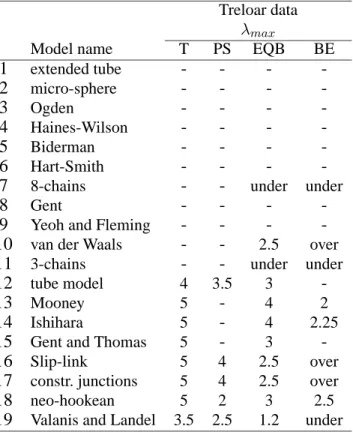
The classification presented in Tables 1 and 2 is es-tablished with the following criteria. The larger is the domain of validity (λmax,λ1 andλ2 for the different

modes of deformation), the upper is the model in the table. Then, the greater is the number of parameters (nop) of the model, lower is the model. For equiva-lent models, more consideration is given to the one which can represent both sets of data with the same set of parameters. Finally, a subjective criterion is taken into account to decide between different equiv-alent models and preferences are awarded to physical-based models (column Phys in Table 2).

Tables 1 gives the limitλmaxof the validity domain

for (T) traction, (PS) pure shear, (EQB) equibiaxial extension and (BE) biaxial extension for identifica-tion on Treloar data. Notaidentifica-tions (under) and (over) in-dicates if stresses are predicted with underestimation or overestimation.

Tables 2 gives limit of the validity domain λmax

in both directions ( λ1 and λ2) for Kawabata et al.

data. Notations (under) and (over) indicates if stresses are predicted with underestimation or overestimation. Symbols (=) or (6=) indicate if only one set of

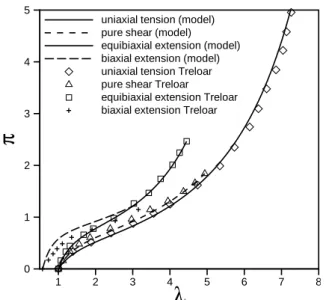
param-eters is able to reproduce both sets of data. 4.3 Example

The following graphs illustrate the performance of the extended tube model. They are obtained with the same set of parameters for both sets of experimental data. The value of these parameters are given with the notations of Kaliske and Heinrich (1999).

5 CONCLUSIONS

This paper focuses on hyperelastic models found in the literature and investigates their capability to re-produce the mechanical behaviour under all kinemat-ically admissible modes of deformation.

Table 1. Classification of hyperelastic models: validity do-main for Treloar data

Treloar data

λmax

Model name T PS EQB BE

1 extended tube - - - -2 micro-sphere - - - -3 Ogden - - - -4 Haines-Wilson - - - -5 Biderman - - - -6 Hart-Smith - - -

-7 8-chains - - under under

8 Gent - - -

-9 Yeoh and Fleming - - - -10 van der Waals - - 2.5 over

11 3-chains - - under under

12 tube model 4 3.5 3

-13 Mooney 5 - 4 2

14 Ishihara 5 - 4 2.25

15 Gent and Thomas 5 - 3

-16 Slip-link 5 4 2.5 over

17 constr. junctions 5 4 2.5 over

18 neo-hookean 5 2 3 2.5

19 Valanis and Landel 3.5 2.5 1.2 under

Table 2. Classification of hyperelastic models: validity do-main for Kawabata et al. data; (nop) number of parameters; (Phys) physical-based model;

Kawabata data

λmax

Model name λ₁ λ₂ nop Phys

1 extended tube = - - 4 × 2 micro-sphere = - - 5 × 3 Ogden 6= - - 6 4 Haines-Wilson 6= 3.4 3 6 5 Biderman 6= 2.5 3 4 6 Hart-Smith = 1.9 1.5 3 7 8-chains 6= 1.9 1.9 2 × 8 Gent 6= 1.6 1.6 2

9 Yeoh and Fleming 6= 1.6 1.6 4

10 van der Waals = 2.2 2.2 4 ×

11 3-chains 6= 1.3 1.3 2 ×

12 tube model = - - 3 ×

13 Mooney 6= 2.2 2 2

14 Ishihara 6= 1.9 1.9 3 ×

15 Gent and Thomas = 1.6 1.6 2

16 Slip-link 6= 2.5 2.5 3 ×

17 constr. junctions 6= 2.2 2.2 3 ×

18 neo-hookean = 1.6 1.6 1 ×

++ ++ ++ + + +

λ

π

uniaxial tension (model) pure shear (model) equibiaxial extension (model) biaxial extension (model) uniaxial tension Treloar pure shear Treloar equibiaxial extension Treloar biaxial extension Treloar

+

Figure 1. comparison between the extended tube model and experimental data of Treloar: Gc = 0.202; Ge = 0.153; β = 0.178; δ = 0.0856 8

λ

π

Figure 2. comparison between the extended tube model and experimental data of Kawabata et al.: Gc = 0.202; Ge= 0_{.153; β = 0.178; δ = 0.0856}

A methodology is proposed to identify the mod-els with previously published experimental data. An identification procedure has been developed. An orig-inal point of this method is the use of genetic algo-rithms coupled to classical optimisation approaches. The proposed method leads to the identification of both material parameters and of the validity domain of the models.

Finally, a classification of the models is proposed considering the domain of validity for all modes of deformation, the number of parameters and the type of formulation used to derive the models. Depending on the considered domain of deformation, the neo-hookean model, the Mooney model and the Ogden model can be used respectively for small, moderate or large strain. Nevertheless, the study highlights non-classically used physical-based models which leads to better agreement with experiments and involves

a smaller number of parameters: the extended-tube model and the micro-sphere model.

REFERENCES

Ambacher, H., H. F. Enderle, H. G. Kilian, & A. Sauter (1989). Relaxation in permanent net-works. Prog. Colloid Polym. Sci. 80, 209–220. Arruda, E. & M. C. Boyce (1993). A three-dimensional constitutive model for the large stretch behavior of rubber elastic materials. J.

Mech. Phys. Solids 41(2), 389–412.

Attard, M. M. & G. W. Hunt (2004). Hyperelastic constitutive modeling under finite strain. Int. J.

Solids Struct. 41, 5327–5350.

Ball, R. C., M. Doi, S. F. Edwards, & M. Warner (1981, August). Elasticity of entangled net-works. Polymer 22, 1010–1018.

Biderman, V. L. (1958). Calculations of rubber parts (en russe). Rascheti na Prochnost, 40. Boyce, M. C. & E. M. Arruda (2000). Constitutive

models of rubber elasticity: a review. Rubber

Chem. Technol. 73, 505–523.

Davet, J.-L. (1985, (3`eme trimestre). Sur les densit´es d’´energie en ´elasticit´e non lin´eaire: confrontation de mod`eles et de travaux exp´erimentaux. Annales des Ponts et

Chauss´ees.

Flory, P. J. (1994). Network structure and the elas-ticity properties of vulcanized rubber. Chem.

Rev. 35, 51–75.

Furukawa, T. & G. Yagama (1997). Inelastic con-stitutive parameter identification using an evo-lutionary algorithm with continuous individu-als. Int. J. Numer. Meth. Engrg. 40, 1071–1090. Gent, A. N. (1996). A new constitutive relation for

rubber. Rubber. Chem. Technol. 69, 59–61. Gent, A. N. & A. G. Thomas (1958). Forms of the

stored (strain) energy function for vulcanized rubber. J. Polym. Sci. 28, 625–637.

Hart-Smith, L. J. (1966). Elasticity parameters for finite deformations of rubber-like materials. Z.

angew. Math. Phys. 17, 608–626.

Heinrich, G. & M. Kaliske (1997). Theoretical and numerical formulation of a molecular based constitutive tube-model of rubber elasticity.

Comput. Theo. Polym. Sci. 7(3/4), 227–241.

Holland, J. H. (1975). Adaptation in natural and

artificial systems. Ann Arbor: University of

Ishihara, A., N. Hashitsume, & M. Tatibana (1951). Statistical theory of rubber-like elastic-ity -iv (two dimensional stretching). J. Chem.

Phys. 19, 1508–1512.

James, A. G., A. Green, & G. M. Simpson (1975). Strain energy functions of rubber. i. character-ization of gum vulcanizates. J. Appl. Polym.

Sci. 19, 2033–2058.

James, H. M. & E. Guth (1943). Theory of the elastic properties of rubber. J. Chem. Phys. 11, 455–481.

Kaliske, M. & G. Heinrich (1999). An extended tube-model for rubber elasticity: stastistical-mechanical theory and finite element implan-tation. Rubb. Chem. Technol. 72, 602–632. Kawabata, S., M. Matsuda, K. Tei, & H. Kawai

(1981). Experimental survey of the strain en-ergy density function of isoprene rubber vul-canizate. Macromolecules 14, 154–162.

Kilian, H. G., H. F. Enderle, & K. Unseld (1986). The use of the van der waals model to eluci-date universal aspects of structuproperty re-lationships in simply extended dry and swollen rubbers. Colloid Polym. Sci. (264), 866–879. Kuhn, W. & F. Gr¨un (1942). Beziehungen zwichen

elastischen Konstanten und Dehnungs-doppelbrechung hochelastischer Stoffe.

Kolloideitschrift 101, 248–271.

Liu, G., X. Han, & K. Lam (2002). A combined genetic algorithm and nonlinear least squares methode for material characterization using elastic waves. Comp. Meth. Appl. Mech.

En-grg. 191, 1909–1921.

Michalewicz, Z. (1996). Genetic Algorithms +

Data Structures = Evolution Programs (Third,

revised and extended Edition ed.). Springer. ISBN 3-540-606776-9.

Miehe, C., S. Goktepe, & F. Lulei (2004). A micro-macro approach to rubber-like materials - part i: the non-affine micro-sphere model of rubber elasticity. J. Mech. Phys. Solids 52, 2617–2660. Mooney, M. (1940). A theory of large elastic

de-formation. J. Appl. Phys. 11, 582–592.

Mullins, L. (1948). Effect of stretching on the properties of rubber. Rubber Chem.

Tech-nol. 21, 281–300.

Ogden, R. W. (1972). Large deformation isotropic elasticity - on the correlation of theory and ex-periment for incompressible rubberlike solids.

Proc. R. Soc. Lond. A 326, 565–584.

Rivlin, R. S. (1948). Some topics in finite elasticity I. Fundamental concepts. Philos. T. Roy. Soc.

A 240, 459–490.

Rivlin, R. S. & D. W. Saunders (1951). Large elas-tic deformations of isotropic materials - vii. ex-periments on the deformation of rubber. Philos.

T. Roy. Soc. A 243, 251–288.

Seibert, D. J. & N. Sch¨oche (2000). Direct compar-ison of some recent rubber elasticity models.

Rubber Chem. Technol. 73, 366–384.

Treloar, L. R. G. (1943). The elasticity of a net-work of long chain molecules (I and II). Trans.

Faraday Soc. 39, 36–64 ; 241–246.

Treloar, L. R. G. (1944). Stress-strain data for vul-canised rubber under various types of deforma-tion. Trans. Faraday Soc. 40, 59–70.

Valanis, K. C. & R. F. Landel (1967). The strain-energy function of a hyperelastic mate-rial in terms of the extension ratios. J. Appl.

Phys. 38(7), 2997–3002.

Wang, M. C. & E. Guth (1952). Statistical theory of networks of non-gaussian flexible chains. J.

Chem. Phys. 20(7), 1144–1157.

Yeoh, O. H. & P. D. Fleming (1997). A new attempt to reconcile the statistical and phe-nomenological theories of rubber elasticity. J.

Polymer Sci. . Part B: Polymer Physics 35,

1919–1931.

Yoshimoto, F., T. Harada, & Y. Yoshimoto (2003). Data fitting with a spline using a real-coded ge-netic algorithm. Comp. Aided Design 35, 751– 760.