HAL Id: hal-01903388
https://hal.laas.fr/hal-01903388
Submitted on 19 Nov 2018HAL is a multi-disciplinary open access
archive for the deposit and dissemination of sci-entific research documents, whether they are pub-lished or not. The documents may come from teaching and research institutions in France or abroad, or from public or private research centers.
L’archive ouverte pluridisciplinaire HAL, est destinée au dépôt et à la diffusion de documents scientifiques de niveau recherche, publiés ou non, émanant des établissements d’enseignement et de recherche français ou étrangers, des laboratoires publics ou privés.
A GPS-less Framework for Localization and Coverage
Maintenance in Wireless Sensor Networks
Imen Mahjri, Amine Dhraief, Abdelfettah Belghith, Khalil Drira, Hassan
Mathkour
To cite this version:
Imen Mahjri, Amine Dhraief, Abdelfettah Belghith, Khalil Drira, Hassan Mathkour. A GPS-less Framework for Localization and Coverage Maintenance in Wireless Sensor Networks. KSII Transac-tions on internet and information systems, 2016, 10 (1), pp.96-116. �10.3837/tiis.2016.01.006�. �hal-01903388�
A GPS-less Framework for Localization and Coverage
Maintenance in Wireless Sensor Networks
Imen Mahjria,b, Amine Dhraiefb, Abdelfettah Belghithc, Khalil Driraa and Hassan Mathkourc
a LAAS-CNRS, University of Toulouse
Toulouse 31400, France
b HANA Lab, ENSI, University of Manouba
Manouba 2010, Tunis, Tunisia
c College of Computer and Information Sciences, Kind Saud University
Riyadh 11543, Saudi Arabia,
Abstract
Sensing coverage is a fundamental issue for Wireless Sensor Networks (WSNs). Several coverage configuration protocols have been developed; most of them presume the availability of precise knowledge about each node location via GPS receivers. However, equipping each sensor node with a GPS is very expensive in terms of both energy and cost. On the other hand, several GPS-less localization algorithms that aim at obtaining nodes locations with a low cost have been proposed. Although their deep correlation, sensing coverage and localization have long been treated separately. In this paper, we analyze, design and evaluate a novel integrated framework providing both localization and coverage guarantees for WSNs. We integrate the well known Coverage Configuration Protocol CCP with an improved version of the localization algorithm AT-Dist. We enhanced the original specification of AT-Dist in order to guarantee the necessary localization accuracy required by CCP. In our proposed framework, a few number of nodes are assumed to know their exact positions and dynamically vary their transmission ranges. The remaining sensors positions are derived, as accurately as possible, using this little initial location information. All nodes positions (exact and derived) are then used as an input for the coverage module. Extensive simulation results show that, even with a very low anchors density, our proposal reaches the same performance and efficiency as the ideal CCP based on complete and precise knowledge of sensors coordinates.
1. Introduction
Wireless sensor networks (WSNs) are an active research and commercial area of interest [1]. A WSN usually consists of a large number of small, low-cost sensor nodes that cooperate with each other to monitor the physical word. Applications of wireless sensor networks are virtually limitless. They include among others, industrial control and monitoring, target tracking and surveillance, home automation and health care. This diversity of applications and domains gives rise to many important issues and requirements that need to be effectively treated during the design of WSN protocols. Sensing coverage and localization are two of the most fundamental and challenging problems in wireless sensor networks.
Sensing coverage reflects how well a sensor network is able to monitor or track a given field of interest. It is considered as one of the most critical measures of performance or service quality offered by a WSN [2]. So far, several sensing coverage protocols have been proposed [3]. Throughout the diversity of research works in this topic, major interests focused purely on the coverage problem under the restrictive assumption that each deployed node is equipped with a GPS receiver that provides it with its precise location. However, in a real life situation, adding a GPS receiver to each deployed node is infeasible and nonpractical for several reasons. First, in a dense network with a large number of nodes, the manufacturing cost of GPS modules is very significant. Moreover, the size of a GPS receiver may be very large for many applications using extremely small sensor devises. Lastly, the power consumption caused by the GPS receiver impact severly the battery lifetime, which is inherently contradictory to the nature of sensor nodes. An alternative solution to GPS is consequently highly needed.
In the meanwhile, several localization algorithms have been proposed to enable sensor nodes to autonomously determine their positions without relying on GPS capabilities [4]. Such algorithms enable sensor nodes to estimate their positions with some degree of precision. Typically, a small number of nodes, called anchors, know their own locations by either human intervention or GPS devices. The remaining majority of nodes, called unknowns, ignore their positions. Based on anchor nodes information, localization algorithms attempt to derive the locations of as many unknown nodes as possible.
In spite of the tight relation between them, sensing coverage and localization protocols have been discussed and evaluated separately. In this paper, we present the design and analysis of a novel framework which treats both sensing coverage and localization in a synchronized way. With this integration, the sensing coverage algorithm will no longer depend on GPS services. We particularly choose to integrate the well-known coverage maintenance protocol CCP [5] with an improved version of the localization algorithm AT-Dist [6]. The original specification of AT-Dist is modified in order to guarantee the necessary localization accuracy required by CCP. Notably, we assume that anchor nodes are able to dynamically increase their transmission range in order to ameliorate positions estimation.
The remainder of the paper is structured as follows. Section 2 reviews related works on sensing coverage and localization in wireless sensor networks. Section 3 gives a detailed description of the Coverage Configuration Protocol CCP and presents some recommendations on how to appropriately set its different parameters. Section 4 explains the Distance Based Approximation Technique AT-Dist. Section 5 describes and studies the performance of the enhanced version of AT-Dist, describes the proposed framework, studies its performance, discusses its potential security threats and shows how to deal with them. Section 6 concludes the paper.
2. Related Works
In the following section, we first detail the sensing coverage strategies in wireless sensors networks. Then, we give an overview of localization algorithms.
2.1 Sensing Coverage
Sensing coverage quantifies how well an area of interest is covered by the deployment of a given sensor network. In the literature, the coverage problem has been formulated in various ways. A location in an area A is said to be covered by a sensor si if it is within the sensing range of si. A location in A is said to
be k-covered if it is covered by at least k (k ≥ 1) sensors. Depending on the coverage objectives and applications, coverage techniques can be classified into three types: point (target) coverage, barrier coverage, and area coverage.
2.1.1 Point Coverage
In the point coverage problem, the objective is to cover a set of discrete points (targets). This type of coverage is mainly used in military applications. In a friendly and an accessible environment, a set of sensor nodes can be deterministically placed to cover the target points. In this way, the objective of a deterministic node placement is to find the minimum number of sensors to be deployed and determine their locations such that the envisioned target points are covered. Several works have focused on the planning of sensor positioning [7-9]. [8] proposed a spanning tree-based algorithm that calculates the optimal nodes placement while maintaining the connectivity of the deployed sensors. First, the algorithm constructs the spanning tree over the set of targets, and then consecutively chooses sensors’ locations on the tree (the vertices or along the edges) that guarantees both coverage and connectivity at each step. In [7, 9], optimization techniques are used to model and solve the node placement problem. In a harsh and a hard-access environment, the only way to deploy a sensor network is through randomly scattering a large number of sensor nodes. For example sensors can be dropped from a plane. In such a deployment, a target point may be unnecessarily covered by more than one single sensor node. In order to reduce the energy consumption and consequently the sensor network lifetime, it would be interesting to switch off the unnecessary nodes. The sensors can be divided into a collection of disjoint sets such that every set can satisfy the coverage requirement. These sets are then successively activated one by one. The objective of this approach is to maximize the number of disjoint sets. [10] presented a theoretical analysis for this approach and then proposed a heuristic for the disjoint set covers computation based on a mixed integer programming formulation.
2.1.2 Barrier Coverage
The concept of barrier coverage was firstly discussed by [11] in the context of robotic sensors. The objective of barrier coverage is to minimize the probability of undetected penetrations across the sensor field. In [12-14], the problem of finding penetration paths is studied. A penetration path is a trajectory spanning from one side to the opposite side of the sensor field. For example, given a deployed network, a defender needs to recognize the path along which an intruder may not be detected and take its appropriate measures. In [13], based on computational geometry and Voronoi diagrams, the authors proposed polynomial algorithms to find the maximal breach path and the maximal support path. On the maximal breach path the chance of detecting an intruder is minimized, however on the maximal support path the chance of detecting an intruder is maximized. In [15-17], the authors studied the concept of k-barrier coverage of a belt region. A belt region is k-barrier covered if any crossing path intersects with the sensing areas of at least k distinct sensors. [15] proposed an efficient algorithm that determines whether a region is k-barrier covered and established a deterministic deployment pattern to achieve k-barrier coverage. [17] introduced new techniques to derive reliable density estimates for achieving barrier coverage.
2.1.3 Area Coverage
The most studied coverage problem is the area coverage problem where the whole area of interest has to be covered. Several works have focused on the area coverage problem. [18, 19] addressed the problem of determining the critical sensor density for complete area coverage. The critical sensor density gives
an estimation of the minimum number of sensors required to achieve the coverage of the entire region. [19] presented a grid strategy to find the number of disks required to cover a given area. [18] designed a set of optimal placement patterns to achieve both coverage and connectivity in 3D sensor networks. Other works addressed the sensor activity scheduling problem [5, 20-22]. In random sensor deployments, the number of deployed nodes is much higher than needed. An energy efficient mechanism in such a redundant deployment is to schedule the activation and deactivation of sensor nodes, allowing redundant node to sleep as long as possible. In [20], the authors proposed to divide the sensors into disjoint sets, such that every set fully covers the monitored area, and then successively activated these sets. The authors of [5, 21, 22] proposed distributed and localized node scheduling algorithms. In such algorithms each node decides upon its state based on its neighbours states and locations. Although the three aforementioned coverage strategies have different objectives (covering a point, a hole area or a path), they all make the same assumptions on the available information about the sensor network. They mainly assume that sensor nodes have their exact geographic location information through on board GPS receivers. The positions of sensor nodes are consequently a basic input for sensing coverage algorithms.
2.2 Localization Techniques
The assumption that all the deployed nodes are provided with GPS supplying them with their exact locations, is often unwarranted. Instead, localization techniques may be used to discover nodes positions. In localization algorithms, a few number of anchor nodes are generally assumed to know their own coordinates (through manual configuration or GPS for instance) and other nodes’ coordinates are derived based on these anchor nodes and some particular node localization techniques. Based on their computational organization and the information required for the positions estimation, localization algorithms can be classified into two ways: centralized vs. distributed or range-based vs. range-free. 2.2.1 Centralized vs. Distributed Localization
Centralized localization algorithms are designed to run on a sufficiently powerful central base station. First, the base station collects the environmental information from the different sensor nodes. Then, based on the collected information, it computes the position of each sensor node and feed them back to respective nodes. Centralized algorithms eliminate the problem of nodes’ computational limitations; whereas they introduce a large communication cost due to transporting data to and from the base station. Hence, centralized algorithms are only suitable for small networks. The Multidimensional Scaling-MAP (MDS-MAP) [23] and the Semi-Definite Programming (SDP) [24] are two popular centralized localization algorithms. In contrast, distributed algorithms are designed to run on each node. Sensor nodes use inter-nodes communications to get their positions in the network. Due to the lack of global information, distributed localization is usually less accurate than the centralized one but it considerably reduces communication costs. The Approximate Point in Triangulation (APIT) [25] and the Distance Vector Hop (DV-Hop) [26] are representative proposals in this category.
2.2.2 Range-based vs. Range-free Localization
Range-based algorithms use internodes distances or angles to estimate nodes’ positions. They use special measurements such as the time of arrival (TOA) [27], the angle of arrival (AOA) [28] and the received signal strength (RSS) [27] to calculate the distance or angle separating two sensors. RSS-based techniques depend on the fact that the radio signal strength attenuates with distance. With the radio attenuation information, a receiving node is able to calculate its distance to the transmitting node. In the TOA-based ranging techniques, the distance separating a receiver from a sender is calculated through multiplying the propagation time by the speed of the signal. AOA-based techniques typically rely on the use of radio or microphone arrays to estimate the angle separating the receiver from the transmitter. The Ad Hoc Positioning System using Angle of Arrival (APS-AOA) [28] and the Distance based Approximation Technique (AT-Dist) [6] are examples of range-based localization algorithms. Range-free localization algorithms make no assumption about the availability of inter-nodes distances
or angles to estimate locations. They instead rely on topology and connectivity information assuming an isotropic network where the hop count between nodes is proportional to their distance. The Centroid [29] and the Convex Position Estimation (CPE) algorithm [24] are examples of range-free localization algorithms. Because of the absence of range information, the positions estimations obtained by the rangefree algorithms are usually less accurate than those obtained by the range-based algorithms. However, on the other hand, range-based techniques are generally more complex.
3. The Coverage Configuration Protocol
The Coverage Configuration Protocol CCP is a distributed area coverage protocol for dense wireless sensor networks [5]. It achieves energy conservation by scheduling redundant nodes to sleep while still preserving the sensing coverage of the entire monitored area. In this section, we give a detailed description of CCP. We first present the K-coverage eligibility algorithm. This algorithm allows a sensor node to autonomously evaluate its eligibility to be in the active state. Then, we describe the state transition of CCP. We finally analyze the impact of the different CCP timers on the algorithm performance and give some recommendations on how to set them appropriately.
3.1 The K-Coverage Eligibility Algorithm
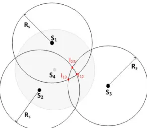
The K-coverage eligibility algorithm is the algorithm that enables a node to decide upon its state: ACTIVE or SLEEP. Given a requested coverage degree K, a node can be in the SLEEP mode if every location within its coverage range is already K-covered by its neighbouring active nodes. For example, in Fig. 1, for K=1, the node S4 can be in the SLEEP mode since its sensing zone is already 1-covered by
the active nodes S1, S2 and S3. In [5] the authors have proved the following theorem:
Theorem 1: A convex region A is K-covered by a set of nodes if (1) it contains intersection points between nodes sensing circles or between nodes sensing circles and A’s boundary;(2) all these intersection points are at least K-covered.
Theorem 1 enables the transformation of the problem of determining the coverage degree of a hole region to the easier problem of determining the coverage degrees of the intersection points within this same region. A sensor is consequently ineligible to turn active if all the intersection points inside its sensing circle are at least K-covered. In Fig. 1, for K=1, node S4 is ineligible to be in the ACTIVE mode
because all the intersection points inside its sensing zone are already 1-covered by the other active nodes in its neighbourhood: the intersection point I23 is covered by the active sensor S1, the intersection point
I13 is covered by the active sensor S2 and the intersection point I12 is covered by the active sensor S3. In
order to find all the intersection points inside its sensing range and check its eligibility, each sensor node needs the location information about all its active sensing neighbours. Therefore, each active node periodically broadcasts messages including its location information.
Fig. 1. An example of 1-coverage eligibility
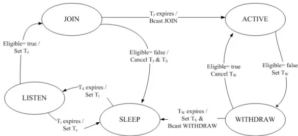
3.2 The CCP State Machine
Nodes running CCP have mainly three operation states: ACTIVE, SLEEP and LISTEN. Each node uses the K-coverage eligibility algorithm to determine its eligibility and dynamically switches its state when its eligibility changes. All nodes are initially in the ACTIVE state. An active node periodically advertises its location and evaluates its eligibility. When a zone exceeds the required coverage degree due to a high density, redundant active nodes will find themselves ineligible and turn into the SLEEP state. A sleeping node periodically wakes up and enters the LISTEN state. During the LISTEN state, a node collects information about its sensing neighbours, re-evaluates its eligibility and decides whether to return to SLEEP mode or to turn into the ACTIVE state. Over time, some nodes may die and create coverage voids. In this situation, some neighbouring nodes in the SLEEP state will find themselves eligible and turn into the ACTIVE mode to cover these voids. As these decisions are done in a distributed way, there could be incompatible state transitions in the neighbourhood. For example, several nodes in the LISTEN state may simultaneously decide to become ACTIVE to cover the same void leading to an unnecessarily redundant coverage. Moreover, several neighbouring active nodes may simultaneously decide to switch to the SLEEP state. In this case, each node will mistakenly believe that its neighbours are still active covering its sensing zone. The coverage degree will consequently decrease below the required level. Two intermediate states JOIN and WITHDRAW are considered to prevent simultaneous transitions from LISTEN to ACTIVE and from ACTIVE to SLEEP, respectively. We describe in the following the detailed state transition rules. Fig. 2 portrays the CCP finite state machine.
ACTIVE State: in the ACTIVE state, the sensor node senses its surrounding environment and transmits information or messages. Moreover, it periodically broadcasts (each Th ) HELLO
messages. When the ACTIVE node receives a HELLO or JOIN message, it evaluates its eligibility to remain active. If it is a redundant node, it starts a withdraw timer Tw and moves to
the WITHDRAW state.
WITHDRAW State: on receiving a WITHDRAW message, the sensor node evaluates its eligibility. If it is no longer ineligible, it cancels the withdraw timer and goes back to the ACTIVE state. If Tw expires and the sensor node is yet ineligible, it broadcasts a WITHDRAW
message, starts a sleep timer Ts and switches the SLEEP state.
SLEEP State: in the SLEEP state, the node turns off its radio to con serve energy. When the sleep timer expires, the node turns on its radio, starts a listen timer Tl, and switches to the
LISTEN State: on receiving a HELLO, JOIN or WITHDRAW message from a neighbour, the eligibility algorithm is executed. If the node is eligible, it starts a join timer Tj and moves to the
JOIN state. Otherwise, on expiration of the listen timer, it sets Ts and goes back to the SLEEP
state.
JOIN State: when a HELLO or JOIN message is received, the sensor node evaluates its eligibility. If it becomes ineligible, it cancels the join timer Tj, sets a sleep timer Ts, and goes
back to the SLEEP state. If Tj expires and the sensor node is yet eligible, it broadcasts a JOIN
message and moves to the ACTIVE state.
Fig. 2. The coverage configuration protocol state diagram
3.3 CCP Timers
The choice of the values of the timers Tw, Tj , Tl, Ts and Th significantly influences the performance of
CCP. In the following, we detail the impact of these timers on CCP.
Withdraw timer (Tw) and join timer (Tj): the withdraw timer and the join timer should be both
randomized in order to avoid contention between several nodes deciding to join or withdraw. Each node randomly and uniformly chooses these timers from the interval [0, max
w T ] and [0, max j
T
], respectively. max wT and
T
jmax, which represent the maximal values of the withdraw and join timers, have to be set according to the network density. In particular, in dense networks the values of maxw
T and
T
jmaxshould be increased to provide nodes with enough time to collect the WITHDRAW or JOIN messages from their crowded neighbourhood. Listen timer (Tl ): the listen timer should be long enough to collect messages from neighbouring
nodes. Among messages, HELLO messages are the most crucial for the K-coverage eligibility algorithm execution. Tl should consequently be set as, Tl=c × Th, where c ≥ 1 is a constant.
Sleep timer (Ts): with a large sleep timer, coverage voids may appear in the network. These
voids can’t be promptly covered due to the extended hibernation of nodes. However, a long sleep timer would conserve nodes energy and consequently increase the network lifetime. With a short sleep timer, the network topology can be very dynamic which may disturb nodes from providing application requirements. Moreover, a shorter sleep duration induces less energy conservation.
Hello timer (Th): the hello timer affects CCP execution time. A short hello timer enables nodes
to rapidly collect neighbours information and decide upon their states. However, a short hello timer means a frequent HELLO messages broadcasting and consequently a high communication overhead.
4. The Distance Based Approximation Technique
The Distance Based Approximation Technique AT-Dist is a distributed, distance based localization algorithm. AT-Dist assumes that all sensor nodes have an identical transmission range R and that each node is able to compute its distances to its neighbours when it receives signals. Nodes running AT-Dist first use the distance estimation technique Sum-Dist to estimate distances to anchors and then approximate their positions using this distance information. In this section we give a detailed description of AT-Dist.
4.1 Sum-Dist
In Sum-Dist every anchor broadcasts a message including its identity, coordinates, and a path length set to zero. Each receiving node calculates the range from the sender (via RSS or TOA), adds it to the path length and broadcasts the message. Hence, each unknown node in the network can obtain a distance estimation and the position of every anchor. Obviously, only the shortest distance will be conserved. If i1,i2,· · ·, in are the intermediate nodes from the anchor a to the unknown node u, then the estimated
distance
dˆ
au between a and u is:iu i i ai au
d
d
d
nd
ˆ
...
2 1 1 (1)Where
dˆ
represents the estimated distance returned by Sum-Dist. For example, in Fig. 3 the estimated distancedˆ
MN between M and N isd
MI
d
IN . By triangular inequality we haveIN MI MN
MN
d
d
d
d
ˆ
.Fig. 3. Principle of distance estimation in Sum-Dist
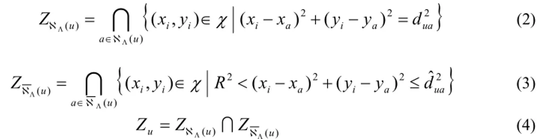
4.2 Positions Estimation
For each anchor a, an unknown node u draws one or two circles:
If u and a are neighbours, then u deduces that it is on the circle centred in a and of radius dau.
If u and a are not neighbours then u deduces that it is not inside the circle centred in a and of radius R. In addition, u knows the estimated distance
dˆ
au. Sinced
au
d
ˆ
au (triangular inequality) then u deduces that it is inside the circle centred in a and of radiusdˆ
au.The intersection of these circles provides a zone Zu containing u. The unknown node u estimates its
position as the centroid of this zone. If we note:
the set of anchors
(u
)
the set of neighbour anchors for an unknown node u
(u
)
the set of non-neighbour anchors for an unknown node u
the set of all possible coordinates in the networkFor each unknown node u, Zu is obtained as follow:
2 2 2
) ( ) ((
i,
i)
(
i a)
(
i a)
ua u a ux
y
x
x
y
y
d
Z
(2)
2 2 2 2
) ( ) ((
i,
i)
(
i a)
(
i a)
ˆ
ua u a ux
y
R
x
x
y
y
d
Z
(3) ) ( ) (u u uZ
Z
Z
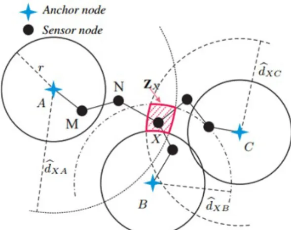
(4) An example is displayed in Fig. 4. The unknown node X first uses SumDist to estimate the distancesXA
dˆ , dˆXBand
dˆ
XC to the different anchors A, B and C. A, B and C are not neighbours of X, X is consequently not inside circles centered respectively at A, B, C and of radius R but it is inside circles of radius dˆXA, dˆXB anddˆ
XC. The correlation of these information defines the red hatched area ZX . XFig. 4. Principle of the localization process in AT-Dis
5. Integrated Localization and Coverage Configuration
In this section, we first describe and study the performance of a new version of AT-Dist. Unlike the original version of AT-Dist which assumes that all sensor nodes have an identical transmission range R, we consider that anchor nodes have a different transmission range than that of unknown nodes. Then, we present our proposed framework: we describe a simple yet an efficient approach for integrating the new version of AT-Dist with CCP to provide both localization and sensing coverage. After, we study the performance of the proposed framework and compare it with the ideal classical case where all nodes are supposed to be equipped with military GPS receivers providing them with their precise coordinates. We finally discuss the security threats that may affect the proposed framework and show how to deal with them.
5.1 AT-Dist With Variable Anchors Range
We propose here to study the performance of AT-Dist under a new specification. Unlike the original specification of AT-Dist [6], we consider two different transmission ranges Ra and Ru. Ra is the anchors
transmission range and is identical among all anchors. Ru is the unknown nodes transmission range and
is identical among all unknowns. Thus, the expression of in Eq(3) becomes:
2 2 2 2
) ( ) ( ( i, i) a ( i a) ( i a) ˆua u a u x y R x x y y d Z
(5)Our simulations are performed using the OMNET++ simulator. We use a square area of 100m × 100m, where 200 nodes are randomly placed using a uniform distribution. Among nodes, we randomly select α anchors with α varying from 2 to 40 which corresponds to a percentage of anchors varying from 1% to 20% respectively. The unknown nodes transmission range Ru is fixed to 14m. Furthermore, we propose
to set the anchors transmission range Ra respectively to 14, 20, 30 and 40m. Each scenario is performed
100 times in order to obtain a small variance. We consider the following metrics:
The average localization error: the average localization error is the sum of the localization errors of all nodes divided by the total number of nodes. Localization errors are normalized to the unknown nodes transmission range Ru. For example an error of 0.5 means that a distance of
half Ru separates the real and the estimated position.
anchors required to reach a given average localization error.
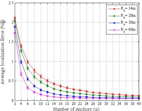
Fig. 5 portrays the average localization error as a function of the anchors used and for different anchor transmission range Ra . There are four curves representing respectively the average localization error
when Ra is equal to 14, 20, 30 and 40m. On the horizontal axis we vary the number of anchors α from 2
to 40. This figure shows that, for the same Ra , the average localization error decreases as the number of
anchors increases. For example, for Ra=20m, the average localization error is of 0.82Ru in a network
containing 6 anchors, it decreases to reach 0.37Ru in a network containing 12 anchors and 0.16Ru in a
network containing 24 anchors. This figure also shows that, for the same number of anchors, the average localization error decreases as the anchors transmission range Ra increases. For instance, for a number of
anchors equals to 10, the average localization error is of 0.61Ru with Ra=14m and it drops to 0.14Ru with
Ra=40m.
Moreover, when comparing two different curves in Fig. 5, for example the curve for Ra=20m and
Ra=40m, we notice that increasing the anchors transmission range has a stronger improvement effect on
the average localization error than increasing the number of anchors. For Ra=20m and with 16 anchors
the average localization error is of 0.25Ru. When doubling the transmission range (i.e., Ra=40m) and
dividing the number of anchors by 2 (i.e.,8 anchors), we reach an improved localization error of 0.20Ru
. This result is expected because the anchors density
Surface
Area
R
D
a a
, linearly increases with the number of anchors and squarely increases with the transmission range.It is also interesting to note that after a certain critical density DC, the average localization error is
slightly improved. If we consider the results for Ra=40m, we notice that the error rate is barely improved
after α=18. Similarly, if we consider the results for Ra=30m, we notice that the average error merely
decreases after α=32. The critical density is consequently 9.0432
100 100 30 32 100 100 40 18
C DIn Fig. 6, we plot the required number of anchors to reach a certain error bound under different anchors communication ranges (Ra=14, 20, 30 and 40m) and different error bounds (Ω=0.05Ru, 0.1Ru,
0.2Ru and 0.4Ru). As expected, for the same error bound Ω, the required number of anchors decreases as
the anchors communication range increases. For example, to reach an average localization error less than or equal to Ω=0.1Ru, we require 48 anchors with a communication range Ra=14m, 35 anchors with
a communication range Ra=20m, 31 anchors with a communication range Ra=30m and only 13 anchors
Fig. 5. Average localization error under different number of anchors α for different anchors transmission ranges Ra
Fig. 6. Required number of anchors under different anchors communication ranges and different error bounds
Overall, previous simulations show the positive effect of increasing the transmission range of AT-Dist anchors. Increasing anchors transmission rangenotably decreases the number of required anchors and increases the localization accuracy.
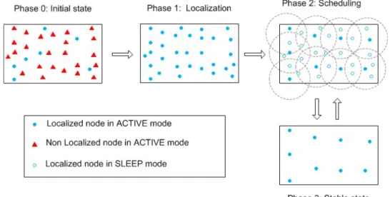
The proposed framework [30] consists in inserting the localization phase just before the scheduling phase. The localization and the scheduling phases are synchronized in a way that active nodes do not participate in the scheduling process until all deployed nodes are well localized. Fig. 7 describes the design of the proposed framework. In the beginning (phase 0), a large number of nodes are randomly dispersed over the area of interest where only a small number of nodes (anchors) are aware of their positions. Then, the localization algorithm is executed (phase 1). At the end of the localization phase, all the deployed sensors are aware of their positions. After that, the scheduling process is applied (phase 2). At the end the scheduling phase, the redundant sensors are set to the sleep mode while the remaining ones stay active to provide a continuous service (phase 3). In static sensor networks, the process periodically turns back to phase 2 and another set of active nodes is chosen. In the case of mobile sensor networks, the process periodically (each Tp) turns back to phase 0 in order to first re-localize sensors and
then choose a new set of active nodes. Tp depends on the mobility of the sensor network. In a highly
mobile sensor network, Tp should be set to a small value in order to have a fresh and accurate
localization. In this paper, we assume that all sensor nodes are static. The proper setting of Tp is left to a
future work.
Fig. 7. Integrated framework for localization and coverage maintenance
5.3 The Framework Performance Evaluation
We implement the proposed framework in the OMNET++ simulator. Sensor nodes are uniformly distributed in a 100m × 100m square area. The deployed number of nodes is 200. The nodes have the same initial transmission range of 14m. The sensing range is fixed to 10m and is identical among sensor nodes. The requested coverage degree is K=1. CCP timers are set as follows: Th =3s, Twmax=
T
jmax=0.5s,Tl = 2 × Th = 6s and Ts = 100s. All experimental results are averages of 100 simulation runs. The
performance metrics of interest are:
The number of active nodes: the number of active nodes is the number of on-duty nodes that the coverage protocol selects to maintain coverage. The lower the number of on-duty nodes is, the better is the ability of the algorithm to conserve energy and consequently to prolong the network lifetime.
area. The coverage is measured as follow: we divide the monitored area into small grids. A grid is considered covered if its centre is covered. The coverage ratio is hence defined as the ratio of the number of covered grids to the total number of grids. A coverage ratio close to 1 indicates the good capacity of the coverage maintenance protocol to preserve the entire area coverage. The achieved coverage degree: the achieved coverage degree is the average coverage degree
of all grids. The coverage degree of a given grid is the number of active nodes covering it. An achieved coverage degree much larger than the required coverage degree K indicates an unnecessary coverage redundancy.
The number of selected active nodes, the coverage ratio and the achieved coverage degree are recorded after the scheduling process is completed. Next, we study the effects of varying the number of anchors as well as the anchors transmission range Raon these metrics.
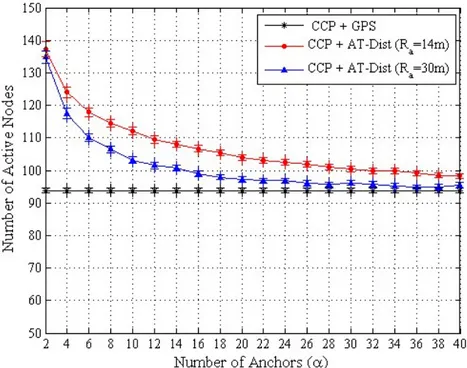
In Fig. 8, we plot the number of active nodes that CCP selects to maintain coverage under each of the two localization techniques GPS and ATDist. Three curves are provided. The curve labeled CCP + GPS represents the number of selected active nodes when each deployed node is supposed to be equipped with a GPS. The curves labeled CCP + AT-Dist represent the number of selected active nodes by the proposed framework (when AT-Dist is used to localize nodes). In this case, the number of anchors is varied from 2 to 40. In the curve CCP + AT-Dist (Ra=30m), during the localization phase, anchor nodes
increase their transmission range Ra from 14m to 30m in order to ameliorate the positions estimations
and then go back to the initial transmission range (i.e., 14m) during the scheduling phase. From this figure, we can see that the use of AT-Dist for localization instead of the GPS leads to an increase in the number of active nodes. This increase is especially observed when AT-Dist uses a small number of anchors. With GPS localization, CCP selects 94 active nodes to maintain the region coverage. With AT-Dist localization, for Ra=30m, CCP selects 135 nodes when 2 anchors are used, that is 40 nodes
more than with GPS localization. The number of active nodes decreases continuously to reach 95 with 28 anchors. This figure also shows that the number of active nodes under AT-Dist localization with Ra=14 is greater than that obtained with Ra=30m. The increase in the number of active nodes is therefore
due to the localization errors induced by AT-Dist. Indeed, the lower is the number of anchors or the anchors transmission range, the poorer are the localization algorithm position estimations. It is important to notice that for Ra=30m and above α=28, which corresponds to anchors density of 7.9 and an
average error of 0.07Ru (Fig. 5), the number of active nodes using AT-Dist localization is almost the
same as that obtained using GPS. This means that, under AT-Dist localization and with an average error less or equal to 0.07Ru , CCP selects the same number of active nodes than with GPS localization. This
result is consistent with the results obtained in papers [31] and [32] where it has been proved that, after a certain bound, localization errors lead to an increase in the number of active nodes.
Fig. 8. Number of active nodes under the two localization techniques GPS and AT-Dist
Fig. 9 plots the coverage ratio provided by CCP under each of the two localization techniques AT-Dist and GPS. From this figure, we notice that CCP is able to provide a good coverage ratio under both AT-Dist and GPS. It keeps a coverage ratio close to 99%. Localization errors have a negligible effect on the coverage ratio. Even with 2 anchors, when the position prediction of AT-Dist is not very precise, the coverage ratio decreases by less than 0.6% in comparison to that obtained by using GPS localization. This result can be explained by the fact that, when CCP uses AT-Dist with a low number of anchors, the number of selected active nodes is more than the necessary (Fig. 8). These redundant active nodes will further cover the monitored area. On the other hand, when CCP uses AT-Dist with an enough high number of anchors, AT-Dist provides sufficiently accurate positions that enable CCP to select the necessary and the exact set of active nodes guaranteeing the monitored area coverage.
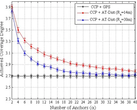
Fig. 10 depicts the achieved coverage degree. From this figure, we can see that the achieved coverage degree using AT-Dist is greater than that using the GPS and this degree decreases as the number of anchors α or the anchors transmission range Ra increases. When CCP uses GPS it achieves a
coverage degree equals to 2.69, however when it uses AT-Dist with Ra=30m it achieves a coverage
degree equals to 3.83 with 2 anchors and 2.72 with 28 anchors. This result conforms to the result obtained in Fig. 8. Indeed, when the number of selected active nodes increases the achieved coverage degree increases accordingly.
Fig. 9. Coverage Ratio under the two localization techniques GPS and AT-Dist
Fig. 10. Coverage degree under the two localization techniques GPS and AT-Dist
In summary, the key results of our experiments are (1) The proposed framework performs well in terms of coverage ratio. It guarantees a coverage ratio close to 99% even with a very low anchors density (2) Beyond a density of anchors of 7.9, the proposed framework can select the same necessary and exact set of active nodes as that selected when GPS localization is used. This density can be easily reached
either by increasing the number of anchors or idealy by just increasing the anchors transmission during the localization phase.
5.4 Security Threats
In our simulations, we have supposed that sensor nodes are deployed in a trusted environment. However, wireless sensor networks are sometimes deployed in harsh and unattended environments, thereby exposing the localization process to several security attacks that may distort the location estimations. An attacker can jam, inject false data and spy on communication. For example, an attacker can erroneously alter the hop counts and the range measurements of the received localization messages or even mimic anchor nodes and broadcast fake locations. In such an untrusted environment, we propose the use of SecAT-Dist [33] the secure version of AT-Dist. SecAT-Dist has the same general localization principle than AT-dist. It secures the localization process by using a lightweight security scheme that combines a RC4-based hash function enabling the authentication of the received location messages and a symmetric encryption system protecting the location information from being selfishly and erroneously altered.
6. Conclusion
Most sensing coverage protocols consider the nodes coordinates as a basic input. Nevertheless, in large sensor networks, straightforward solution of embedding a GPS receiver into each sensor node is not feasible. Coverage algorithms can alternatively rely on localization algorithms. In fact, such algorithms are cost effective, easily to deploy and can operate in various environments.
In this paper, we proposed an integrated localization and area coverage configuration protocol. In sharp contrast to several existing approaches that addressed the two problems separately, we designed a novel framework where we integrated an improved version of the localization algorithm AT-Dist with the coverage maintenance algorithm CCP. With this unification, CCP will no longer rely on GPS to localize sensors. AT-Dist will self-localize the sensor network and supply CCP with the needed location information. To study the efficiency of the proposed framework, we compared it with the ideal classic situation where each networked sensor is equipped with a military GPS providing it with its precise coordinates. Simulation results proved the effectiveness of the framework to provide guaranteed coverage and localization. Indeed, beyond a certain anchors density, the proposed framework reaches the same performance as the ideal case (i.e., each deployed node is aware of its accurate position). To reach this density with a low number of anchors, we proposed to let anchors increase their transmission range during the localization phase and then go back to their initial transmission range during the scheduling phase. Moreover, we addressed the security threats that may encounter the framework in an untrusted environment and proposed the use of a secure version of AT-Dist in order to deal with such threats. Our study indicates that coverage protocols are able to perform very well with the help of even a simple localization algorithm. Localization algorithms can indeed be an excellent and useful alternative to GPS localization. It is consequently appropriate and beneficial to integrate localization and coverage protocols. Integrating these protocols helps to avoid the impracticality and the inaccessibility of the GPS service.
References
[1] S. Misra, I. Woungang, and S.C. Misra, Guide to wireless sensor networks, Springer, 2009.
[2] H. Zhou, T. Liang, C. Xu, and J. Xie, “Multiobjective coverage control strategy for energy-efficient wireless sensor networks,” International Journal of Distributed Sensor Networks 2012, 2012.
[3] B. Wang, “Coverage problems in sensor networks: A survey,” ACM Computing Surveys (CSUR), vol. 43, no. 4, pp. 32, 2011.
[4] S. Biaz and Y. Ji, “A survey and comparison on localisation algorithms for wireless ad hoc networks,” International Journal of Mobile Communications, vol. 3, no. 4, pp. 374-410, 2005.
[5] G. Xing, X. Wang, Y. Zhang, C. Lu, R. Pless, and C. Gill, “Integrated coverage and connectivity configuration for energy conservation in sensor networks,” ACM Transactions on Sensor Networks (TOSN), vol. 1, no. 1, pp. 36-72, 2005.
[6] C. Saad, A. Benslimane, and J. König, “At-dist: A distributed method for localization with high accuracy in sensor networks,” International journal Studia Informatica Universalis, Special Issue on’Wireless Ad Hoc and Sensor Networks, vol. 6, no. 1, 2008.
[7] I.K. Altınel, N. Aras, E. Güney, and C. Ersoy, “Binary integer programming formulation and heuristics for differentiated coverage in heterogeneous sensor networks,” Computer Networks, vol. 52, no. 12, pp. 2419-2431, 2008.
[8] K. Kar and S. Banerjee , “Node placement for connected coverage in sensor networks,” Modeling and Optimization in Mobile, Ad Hoc and Wireless Networks, 2003.
[9] J. Wang and N. Zhong, “Efficient point coverage in wireless sensor networks,” Journal of Combinatorial Optimization, vol. 11, no. 3, pp. 291-304, 2006.
[10] M. Cardei and D.Z. Du, “Improving wireless sensor network lifetime through power aware organization,” Wireless Networks, vol. 11, no. 3, pp. 333-340, 2005.
[11] D.W. Gage, “ Command control for many-robot systems,” in Proc. of the Nineteenth Annual AUVS Technical Symposium, pp. 22-24, 1992.
[12] L.S. Huang, H.L. Xu, Y. Wang, J.M. Wu, and H. Li, “Coverage and exposure paths in wireless sensor networks,” Journal of Computer Science and Technology, vol. 21, no. 4, pp. 490-495, 2006.
[13] S. Meguerdichian, F. Koushanfar, M. Potkonjak, and M.B. Srivastava, “Coverage problems in wireless ad-hoc sensor networks,” in Proc. of the twentieth Annual Joint Conference of the IEEE Computer and Communications Societies, pp. 1380-1387, 2001.
[14] D.P. Mehta, M.A. Lopez, and L. Lin , “Optimal coverage paths in ad-hoc sensor networks,” in Proc. of the IEEE International Conference on Communications, vol. 1, pp. 507–511, 2003.
[15] S. Kumar, T.H. Lai, and A. Arora, “Barrier coverage with wireless sensors,” in Proc. of the 11th annual international conference on Mobile computing and networking, pp. 284–298, 2005.
[16] B. Liu, O. Dousse, J. Wang, and A. Saipulla , “Strong barrier coverage of wireless sensor networks,” in Proc. of the 9th ACM international symposium on Mobile ad hoc networking and computin,. pp. 411-420, 2008. [17] P. Balister, B. Bollobas, A. Sarkar, and S. Kumar, “Reliable density estimates for coverage and connectivity
in thin strips of finite length,” in Proc. of the 13th annual ACM international conference on Mobile computing and networking, pp. 75-86, 2007.
[18] X. Bai, C. Zhang, D. Xuan, J. Teng, and W. Jia, “Low-connectivity and full-coverage three dimensional wireless sensor networks,” in Proc. of the tenth ACM international symposium on Mobile ad hoc networking and computing, pp. 145-154, 2009.
[19] M. Franceschetti, M. Cook, and J. Bruck, “A geometric theorem for wireless network design optimization,” Caltech University, Pasadena, CA, Paradise Tech. Rep, 2002.
[20] S. Slijepcevic and M. Potkonjak, “Power efficient organization of wireless sensor networks,” in Proc. of the IEEE International Conference on Communications, vol. 2, pp. 472-476, 2001.
[21] D. Tian and N.D. Georganas, “A coverage-preserving node scheduling scheme for large wireless sensor networks,” in Proc. of the 1st ACM international workshop on Wireless sensor networks and applications, pp. 32-41, 2002.
[22] H. Zhang and J.C. Hou, “Maintaining sensing coverage and connectivity in large sensor networks,” Ad Hoc & Sensor Wireless Networks, vol. 1, no. 1-2, pp. 89-124, 2005.
[23] Y. Shang, W. Ruml, Y. Zhang, and M.P.J. Fromherz, “Localization from mere connectivity,” in Proc. of the 4th ACM international symposium on Mobile ad hoc networking and computing, pp. 201-212, 2003. [24] L. Doherty, K. S. J. Pister, and L. El Ghaoui, “Convex position estimation in wireless sensor networks,” in
Proc. of the twentieth Annual Joint Conference of the IEEE Computer and Communications Societies, vol. 3, pp. 1655-1663, 2001.
[25] D. Niculescu and B. Nath, “Ad hoc positioning system (aps),” in Proc. of the IEEE Global Telecommunications Conference, vol. 5, pp. 2926-2931, 2001.
[26] T. He, C. Huang, B.M. Blum, J.A. Stankovic, and T. Abdelzaher, “Range-free localization schemes for large scale sensor networks,” in Proc. of the 9th annual international conference on Mobile computing and networking, pp. 81-95, 2003.
[27] B. W. Parkinson and J. J Spilker, Progress In Astronautics and Aeronautics: Global Positioning System: Theory and Applications, Aiaa, 1996.
[28] D. Niculescu and B. Nath, “Ad hoc positioning system (aps) using aoa,” in Proc. of the 7th twenty-Second Annual Joint Conference of the IEEE Computer and Communications, vol. 3, pp. 1734-1743, 2003.
[29] N. Bulusu, J. Heidemann, and D. Estrin, “Gps-less low-cost outdoor localization for very small devices,” IEEE Personal Communications, vol. 7, no. 5, pp. 28-34, 2000.
[30] I. Mahjri, A. Dhraief, I. Mabrouki, A. Belghith and K. Drira, “The Coverage Configuration Protocol under AT-Dist Localization,” in Proc. of the 5th International Conference on Ambient Systems, Networks and Technologies (ANT-2014), Procedia Computer Science, vol. 32, pp. 141-148.
[31] A. Dhraief, I. Mahjri, and A. Belghith, “A performance evaluation of the coverage configuration protocol under location errors, irregular sensing patterns, and a noisy channel,” International Journal of Business Data Communications and Networking, vol. 8, no. 3, pp. 28-41, 2012. http://dx.doi. org/10.4018/jbdcn.2012070102
[32] A. Dhraief, I. Mahjri, and A. Belghith, “A performance evaluation of the coverage configuration protocol and its applicability to precision agriculture,” Multidisciplinary Perspectives on Telecommunications, Wireless Systems, and Mobile Computing, pp. 107-122, 2014.
[33] A. Abdelkarim, A. Benslimane, I. Mabrouki, and A. Belghith, “Secat-dist: A novel secure at-dist localization scheme for wireless sensor networks,” IEEE Vehicular Technology Conference, pp. 1-5, 2012.