Evaluation of the topographic effect on the results of mapping by electrical resistivity method: application to rubber tree plantation on Ban Non Tun experimental site in north-east of Thailand

HAL Id: hal-00794616

https://hal.archives-ouvertes.fr/hal-00794616

Submitted on 26 Feb 2013

HAL is a multi-disciplinary open access

archive for the deposit and dissemination of sci-entific research documents, whether they are pub-lished or not. The documents may come from teaching and research institutions in France or abroad, or from public or private research centers.

L’archive ouverte pluridisciplinaire HAL, est destinée au dépôt et à la diffusion de documents scientifiques de niveau recherche, publiés ou non, émanant des établissements d’enseignement et de recherche français ou étrangers, des laboratoires publics ou privés.

Evaluation of the topographic effect on the results of

mapping by electrical resistivity method: application to

rubber tree plantation on Ban Non Tun experimental

site in north-east of Thailand

Sylvain Pasquet

To cite this version:

Sylvain Pasquet. Evaluation of the topographic effect on the results of mapping by electrical resistivity method: application to rubber tree plantation on Ban Non Tun experimental site in north-east of Thailand. 2011. �hal-00794616�

NRCT-06

Office of the National Research Council of Thailand (NRCT)

Office of International Affairs

196 Phaholyothin Road

Chatuchak, Bangkok 10900, Thailand

Phone: +(66-2) 940-6369, 579-2690 Fax: +(66-2) 561-3049

Website : www.nrct.net, www.nrct-foreignresearcher.org

E-mail : webmaster@nrct-foreignresearcher.org

COMPLETE REPORT SUBMISSION FORM

Please type or print in English

RESEARCH PROJECT TITLE:

Evaluation of the Topographic Effect on the Results

of Mapping by Electrical Resistivity Method: Application to Rubber Tree

Plantation on Ban Non Tun Experimental Site in North-East of Thailand

1. Name:

Sylvain

Eric

PASQUET

(First)

(Middle)

(Last)

2. Foreign researcher registration no.:

21/54

3. Current employer:

IRD

Address:

IRD, LDD, Office of Science for Land Development 2003/61,

Phahonyotin Rd., (next to soi 41), Chatuchak, BANGKOK

Postal code:

10900

Country:

Thailand

Phone:

(+66) 25 61 27 28 #0

Fax:

(+66) 25 61 21 86

E-mail:

pasquet.syl@gmail.com

4. Research duration: Starting:

04/04/2011

Ending:

19/09/2011

D M Y

D M Y

5. Checklist for complete report submission. These sections are to follow this

submission form.

[x] Executive summary

[x] Acknowledgment

[x] List of collaborating Thai researchers and/or Thai institutions

[x] Background and rationale

[x] Objective of research

[x] Research methodology

[x] Research results

[x] Conclusions and recommendations

[x] References

[ ] Appendices (if necessary)

I do hereby certify that all of the above given checks are true.

(Foreign researcher’s signature)

07/09/2011

(Date)

Project I.D.

2

1 E

XECUTIVE SUMMARY

Since 1991, Thailand has been the largest country in the world for natural rubber production and its export. More than 80% of Thailand natural rubber is produced by smallholders. It is obvious that the production of natural rubber has a very important economic interest. For rubber-tree, the normal climatic and environmental conditions are: mean annual temperature of 26°C ± 2°C, and high rainfall (from 1800 to 3000 mm/year) regularly distributed throughout the year (with 120 - 240 rainy days per year) [Gonçalves et al., 1999].

Worldwide demand for natural rubber is increasing every year and so is its price in the world market. In addition of this, the governmental subsidizations in Thailand have created beneficial conditions for the expansion of rubber-tree (called “hevea”) plantations even in areas where climatic conditions are not really auspicious for this plant. This applies to the NE of Thailand and particularly in the Khon Kaen region, characterized by a semi-arid tropical climate where the annual average air temperature is 26°C and the total precipitation does not exceed 1300mm/year, almost all of it falling during the rainy season from April to October [Watanabe & al., 2004]. If the temperature is favorable for rubber-tree growth, the rainfall remains below the requested moisture and its distribution is irregular.

The effects of water deficiency or excess can lead to reduced rates of tree growth, low latex yields [Rao et al., 1998], and in severe cases, the water stress may affect the plantations resulting in “hevea” diseases or total plant failure. In this area the sandy soils are not rich in organic matters and other nutrients. For this region the soil and the climate can be considered as marginal for rubber-tree cultivation. Traditional management of intensive cropping in this area should include specific studies on soil - water – plant - atmosphere interactions. Failure to do so could cause irreversible damage. An increase in rubber-tree plantation surfaces in the long term can lead to important changes of water resources and no foreseeable impact on soils. Several scientists from different professional fields are working for many years to find and propose solutions to grow this tree in the described above conditions. The ongoing TICA project "Impact assessment of planting rubber trees on sandy soils in NE Thailand, Phase 2 " (started since September 2010, for 3 years), which is a cooperation project between the Land Development Department of Thailand and the French Research Institute for Development (IRD), has for purpose to contribute to the strategy of LDD, particularly by studying the soil variability and find solution in rehabilitation of marginal up-lands of North-East Thailand in order to enlarge the area of rubber-tree plantations and to improve living conditions for Thai smallholders. In order to study the soil variability on the experimental site “Ban Non Tun”, an electrical resistivity mapping was carried out. This map showed that the lines of trees are characterized by resistant anomalies compared with "interline" zones. But it is not obvious to link these anomalies directly with the root systems of trees, because between the "lines of trees" and the "interlines" exists a topographical unevenness specially created by the farmer to protect trees roots from water excess during rainy periods. Under these conditions, the differences in elevation between the "lines" and "interlines" may themselves generate apparent electrical resistivity anomalies, even when the ground is homogeneous. In this case, we have at least two sources that can create anomalies in the same direction (resistivity increasing).

The conceptual framework of this project includes a detailed analysis of the apparent electrical resistivity anomalies in order to estimate the contributions from various sources. A comparison of

3

data measured in the field with those of modeling allows us to assess the topographic effects on electrical resistivity values obtained by mapping.

Several studies have been done concerning the influence of topography on the electrical resistivity measurements [Fox et al., 1980], but the proposed approaches and correction methods are difficult to apply for the site “Ban Non Tun”, due to very inhomogeneous distribution of soil's electrical resistivity and topographical irregularities.

This project aims to estimate the contribution of different sources that can generate these anomalies. The influence of topographic structures on the apparent electrical resistivity measurements is evaluated using numerical calculations. Field detailed measurements, using different electrode configurations, assesses the degree of adaptation of different arrays for geophysical surveys in rubber tree plantations. It also helps for a deeper understanding of phenomena, and a better interpretation of the results of electrical resistivity mapping.

Comparison of the Ban Non Tun site topographic map and electrical resistivity mapping shows a clear coherence between ranks of trees and extended resistant anomalies. More detailed topographic and electrical resistivity mapping have been done on a small surface in order to better identify the sources of the anomalies observed on the electrical resistivity mapping. This area, centered on a rank of trees, includes both extended resistant anomalies and a conductive anomaly on the topographic structure.

Results of apparent electrical resistivity mapping obtained using the "pole-pole", "Wenner-α" and "dipole-dipole" arrays with the same inter-electrode spacing were compared to study the probable differences between responses observed on the same structures.

We used results obtained in pole-pole configuration with an inter-electrode spacing of 25 cm to calculate the index of anisotropy in the horizontal plane. Index values are on average very close to 1, which shows that the topographical effect is very small compared to the influence of superficial layers resistivities.

Raised portions of relief corresponding to the ranks of trees were established by extracting soil in the inter-ranks areas to transfer it on the lines of tree. This has certainly led to a significant deterioration of the structure of these soils, which could result in an increase in their electrical resistivity.

Results of topographic effect modeling show consistent resistant anomalies corresponding to the topographic structure. Yet, amplitudes of these anomalies (around 5-10 %) are lower than those observed on the site (more than 150 %). Thus, the topographic effect cannot be the only source of the extended resistant anomalies observed on the results of electrical resistivity mapping on the “Ban Non Tun” site.

These results allow us to improve our knowledge concerning sources and physical bases of the recorded resistive anomalies along the ranks of trees.

4

2 A

CKNOWLEDGMENTS

This research project would not have been possible without the support of many people. I wish to express my gratitude to NRCT for allowing me to carry out my internship in Thailand. I also would like to thank all the LDD and the Office of Science for Land Development in Bangkok for their collaboration and hospitality, with particular thanks for Dr. Im-Erb Rungsun and Khun Nopmanee Suvannang for their constructive advises.

I would like to convey my thanks to my colleagues from IRD and CIRAD, and especially to Marine Souchier, for supporting me in achieving this innovative internship project. Also not forgetting Khun Amphawan Choosaeng, Khun Jiraporn Mahaphann, Khun Khruawan Panjam and Hans-Gerhard Nehring for being so patient and helping me with all the administrative procedures.

My thanks to all the Thai teachers and student I met for their constant availability and kindness, and especially Dr. Vidhaya Trelo-Ges and Khun Weerachon Sakphong from Khon Kaen University, Khun Jaruwan Saengsri and Khun Pranutkun Sungwalwong from Kasetsart University, and Khun Jessada Sopharat and Khun Sakanam Lim from Prince of Songkla University.

Deepest gratitude is due to my supervisor, Dr. Gaghik Hovhannissian, who believed in me from the very beginning and offered me invaluable advices, support and guidance all along these six months. This internship wouldn’t have been possible without his tenacity to obtain acceptance for the project.

Finally, I would like to thank our Thai assistants, and especially Khun Kasem Posri and Khun Weerawut Yotjamrut, for their constant desire to help and improve the work conditions in any kind of situation. Very special thanks to Khun Worraphan Chintachao and Khun Ratchapol Siriboon for helping me in the field, sharing with me their knowledge concerning Thai country, customs and language, and especially for having been there for me at all time.

3 L

IST OF COLLABORATING

T

HAI RESEARCHERS AND

/

OR

T

HAI INSTITUTIONS

Land Development Department, Office of Science for Land Development

1. Khun Nopmanee Suvannang (Office of Science for Land Development, LDD - Bangkok) 2. Dr. Wanphen Wiriyakitnateekul, (Office of Science for Land Development, LDD - Bangkok) 3. Dr. Im-Erb Rungsun, (Land Development Department, Bangkok)

4. Khun Siwaporn Siltecho (Land Development Department, Region 5 - Khon Kaen) Khon Kaen University, Faculty of Agriculture, Department of Land Resources & Environment

1. Dr. Vidhaya Trelo-Ges (Associate Professor)

2. Khun Ratchapol Siriboon (Master’s degree student) 3. Khun Weerachon Sakphong (Master’s degree student)

5

4 B

ACKGROUND AND RATIONALE

4.1 I

During the 60-70’s, the North East of Thailand, mostly covered with natural forests, has seen its perennial tree cover to be replaced by annual crops (rice, maize, sugarcane, cassava). Sandy soils of this region, fragile with low organic matter content, were heavily damaged by water and wind erosion induced by deforestation. This also led to a rise of the deep aquifer level, causing soil salinization which gradually made them barren [Williamson D.R. et al., 1989]. The massive use of fertilizers and various chemicals also contributed to this ecological issue.

In the late 80’s - early 90's, the Thai governmental institutions, and particularly the Land Development Department (LDD), have addressed this problem to find remedial solutions ensuring growth of agricultural productivity, increase of farmers' incomes and preservation of the environment. The LDD, long-time partner of the Institut de Recherche pour le Développement (IRD), is a governmental agency coming under the authority of the Ministry of Agriculture. It is responsible for land planning, reorganization of agricultural land use, resource conservation, and advises farmers on these topics. The scientific cooperation project between LDD and IRD "Impact assessment of planting rubber trees on sandy soils in NE Thailand, Phase 2" is designed to study the specific conditions of rubber tree cultivation in Northeast Thailand and offer new approaches for the use of land and water resources in order to increase both production of natural latex and farmers' incomes. To meet a fast-growing global demand for paper and natural rubber, the Thai government decided to subsidize development of rubber trees and eucalyptus plantations in the Northeast of Thailand. Since 1991, Thailand has become the largest producer and exporter of natural rubber. Over 80% of this production is provided by owners of small plantations (less than 10 ha), it is thus necessary to protect and develop this economic sector.

Southern Thailand has climatic and environmental conditions similar to the Amazon, where the rubber trees originally grow. The average temperature is 26°C ± 2°C with rainfall of 1800-3000 mm/year distributed regularly throughout the year (120 to 240 days of rain per year) [Gonçalves et

al., 1999]. The Northeast of Thailand, and especially the Khon Kaen region, is characterized by a

semi-arid tropical climate, far from these conditions. If the temperature is favorable to the growth of rubber trees (26°C on average), rainfall are low and very irregular (1300-1400 mm/year on average, distributed mainly between April and October) [Watanabe et al., 2004]. This irregularity can cause an extended lack or excess of water that can slow down tree growth and reduce the latex production [Rao et al., 1998]. In severe cases, these water crises can cause illness or death of the tree.

4.2 D

B

N

T

(BNT

2)

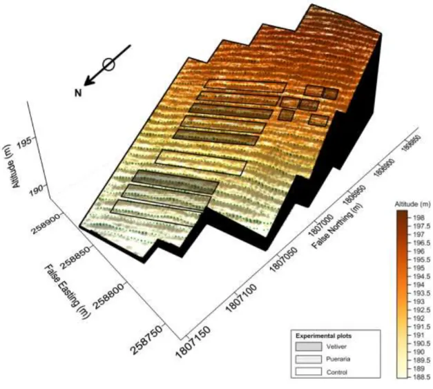
The experimental site of Ban Non Tun is located about 20-25 km southwest of Khon Kaen city and covers an area of 3.75 ha with an irregular pentagon shape outstretched in the NS direction. The altitude difference between the southern (upstream) and the northern (downstream) parts is slightly more than 10 m with slopes between 2 and 5 %. This surface is curved, with the central part of the site higher than the lateral areas (Figure 1).

6

Figure 1 : Topographic map of the Ban Non Tun site with position of the trees (green dots).

This site presents a rubber tree plantation where the trees are planted every 2.5 m along ranks spaced apart by 7 m. The ranks are slightly elevated compared with inter-ranks. These structures were created by the owner to protect tree roots from excess of water during the rainy season. For agronomic experiments, plots of Pueraria and Vetiver have been installed on some inter-ranks areas.

Pueraria plots are intended to naturally increase soil fertilization with nitrogen exchanged between

the plant and the soil during its degradation, while Vetiver plots are used to reduce the impact of water excess due to the plant’s very long roots. The vegetation of these plots also offers protection to the soil against wind and water erosion. The growth of all trees is followed by regular measurements (twice a year) of their circumference at a constant height (h = 1.40 m from the ground). More frequent observations (monthly) are done along the ranks of trees in the middle of each experimental plot.

A data logger records information coming from hydrological and geophysical sensors installed on a central transect following the slope, and from two weather stations located upstream and downstream.

Geophysical measurements on this site are intended to study the characteristics of agronomic experimentation in relation with the soil spatial variability.

7

4.3 G

Various geophysical methods were used to study the soil spatial variability. With these non-destructive methods, we can obtain quick detailed mapping of soils, unlike traditional approaches of Soil Science (auger soundings, piezometers, tensiometers, neutron probes ...) that provide only localized spatial information.

Three geophysical methods were used in Ban Non Tun:

 Electrical resistivity mapping (RM15)

 Spontaneous potential mapping (SP)

 Electrical resistivity tomography (ERT)

The electrical resistivity mapping methodology provided maps of the spatial variability of soil electrical properties corresponding to three different depths of investigation (0.5, 1 and 2 m). The results of several studies show that soils electrical properties are related to its physical and chemical characteristics (morphology, texture, water and clay content, salinity, presence of pollutants...) [Samouëlian et al., 2005; Tabbagh et al., 2000; Moeys et al., 2006]. The electrical resistivity can therefore be an efficient parameter to characterize the soil spatial variability.

SP mapping is based on the study of natural electrical potentials (or spontaneous) generated in the soil by physical and electrochemical phenomena such as fluid flows in porous media (electrokinetic potential), ions concentration gradients (diffusion potential) or redox processes (mineralization potential) [Hovhannissian et al., 2002; Pinettes et al., 2002]. These natural potentials are measured using a voltmeter and two unpolarizable electrodes implanted in the soil. The application of this method is simple, quick and useful for the recognition of surface heterogeneities. It provides phenomenological and qualitative information on the soil properties. In general, this method is coupled with other geophysical methods to ease interpretation of obtained results.

Electrical Resistivity Tomography (ERT) provides the distribution of apparent electrical resistivity values in a vertical plane along a profile of electrodes implanted at the soil surface. Measurements are done with a Syscal Pro 72 electrodes. This equipment can perform automatic sequences by choosing different pairs of electrodes for injection and measurement. We can thus represent the observed apparent electrical resistivity values on a pseudo-section in depth.

4.4 A

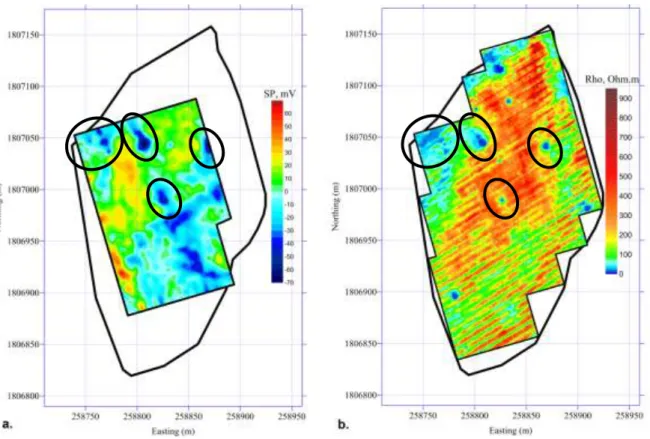
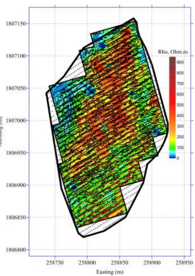
As part of the collaboration project IRD - LDD, SP mapping (Figure 2.a.) was conducted on the experimental site of Ban Non Tun at the beginning of 2010 (January-February). It was followed by an apparent electrical resistivity mapping - ρa (Figure 2.b) at the end of that year (October-November). The general dynamic of the spontaneous potential values on this normalized map has a range of ± 70 mV. The map of electrical resistivity shows significant heterogeneities of the observed values (from 20 to 1000 Ohm.m), with very localized conductive anomalies (about 50 Ohm.m).

8

Figure 2 : Maps of spontaneous potential (a.) and apparent electrical resistivity for a = 0.5 m (b).

The comparison of these two maps highlighted ρa and SP anomalies corresponding to the same locations on the site (marked by ellipses). Conductive anomalies with ρa of about 20 Ohm.m correspond to strongly negative SP anomalies (-50 to -70 mV). The observation in the same places of negative anomalies of the spontaneous potential and low resistivity can be explained by the presence of wet clay in the soil. In general, they are negatively charged on their surface and can be the source of the negative electrical potential measured by the SP method. The clays are also known for their high water holding capacity. The water in the soil is naturally rich in ions and can generate a higher electrical conductivity (or lower resistivity) compared to the surrounding environment (sandstone, sand ...).

The results of several auger soundings in the locations of these anomalies confirm the presence of clays in the soil surface (between 15 and 30 cm deep). In other places, clays appear only in the deep layers or near the alteration zone of the bedrock.

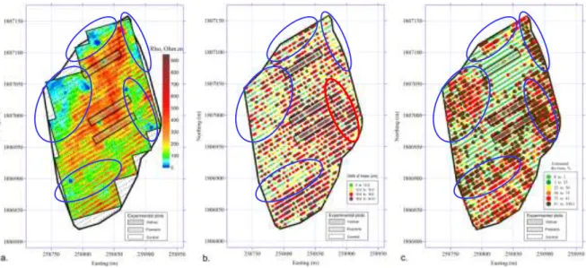
A comparison of tree circumferences (Figure 3, b) measured in September 2009 with the distribution of apparent electrical resistivity (map with a = 0.5 m, Figure 3, a.) shows a general trend of tree slow growth in less resistant areas. Only a relatively high growth of trees planted on a conductive zone located east of the site (red ellipse) is in contradiction with this trend. A thorough study of this area is expected to understand this difference.

Rubber trees planted in plots of Pueraria are mainly characterized by large diameters. This particularly high growth is probably related to the high concentration of nitrogen in the soil, consequence of the agronomic experimentations.

9

Figure 3 : Comparison of the apparent electrical resistivity map (a.) with the results of agronomic observations (b. circumferences - c. state of trees).

The natural growth of trees has been disturbed by a water crisis due to a long period without significant rainfall between October 2009 and June 2010 (Figure 4). In 2007, observed values corresponded to the average annual rainfall characteristics of the region (about 1300 mm) whereas 2008 was characterized by higher rainfall (more than 1900 mm), followed by a large deficit of rainfall during the year 2009 (only 1170 mm). These extreme weather conditions caused extensive damage to trees in this plantation, leading to their partial or complete drying.

Figure 4 : Rainfall in Ban Non Tun between 2007 and 2010.

In July 2010, an observation of the state of each tree was conducted to assess the damages. To represent the degree of damage of trees on a map, they were classified according to the following criteria:

 non-damaged trees - 0%;

 partially damaged trees characterized by the ratio between the number of dry branches and the total number of branches, expressed as a percentage;

 trees whose top is completely dry and with new branches in the lower part of the trunk - 80%;

 trees completely dry - 100%.

The results of this observation (Figure 3.c) were compared with the distribution of apparent electrical resistivity (Figure 3.a). Highly damaged trees are located in less resistant areas. We can also note the large number of damaged trees in both Pueraria plots located further south.

10

From the perspective of the interaction between plants and soil, damaged trees corresponding to less resistant areas may be explained by the presence of clays in the soil. Under conditions of low humidity, high water holding capacity of clay can disrupt the normal functioning of tree roots.

Severely damaged trees located on Pueraria plots had higher growth. They therefore needed a larger quantity of water for their normal growth. The high density of Pueraria roots close to those of rubber trees may have created a strong competition between the two plants under conditions of low humidity and thickness of soil (Figure 5).

Electrical Resistivity Tomography reveals a greater thickness of soil corresponding to the plot located north of the site (left side on Figure 5). Most likely, the positioning in the downstream portion of the site is at the origin of more favorable conditions (water, soil thickness and texture) to the growth of rubber trees, which also explains why the trees resisted better to the water crisis.

Figure 5 : Electrical resistivity model obtained by ERT on the Ban Non Tun site in the SN direction.

Consistencies between agronomic observations, soil surveys and spatial variations of the apparent electrical resistivity show the quality of this parameter to characterize soil spatial variability. The results of ρa mapping corresponding to three different depths of investigation (Figure 6) reveal resistant anomalies extended along the ranks of trees. However, it is not easy to give a comprehensive explanation for these anomalies. In the case of the Ban Non Tun site, several sources may cause these anomalies (topography, soil texture and structure, functioning of the tree root system...).

11

5 O

BJECTIVE OF RESEARCH

The main objectives of my internship project are:

• participation to the realization of a detailed topographic map of the “Ban Non Tun” experimental site to compare with electrical resistivity mapping of the total surface;

• evaluation of the topographic effect on electrical apparent resistivity measurements by numerical modeling with "COMSOL" software and using real parameters defined on the experimental site;

• realization of electrical apparent resistivity detailed mapping to compare with modeling results;

• elaboration of appropriate techniques to separate anomalies from different sources and contributing to better interpretation of acquired results by electrical resistivity mapping.

6

RESEARCH METHODOLOGY AND RESULTS

6.1 T

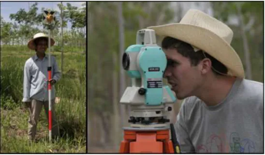
I participated actively in the realization of a detailed topographic map to make a careful comparison between topographic and electrical resistivity maps. We chose a resolution of 4 x 1 m for this map, i.e. more than 10 000 measurement points corresponding to the positions of the electric apparent resistivity (hereafter called ρa) measuring device. Topographical survey was performed with a Nikon Total Station DTM-332 (Figure 7). The applied methodology allowed us to perform measurements with a precision of less than 0.10 m in the horizontal plane and below 0.05 m for the altitude Z.

12

An overlay of elevation contour lines and the apparent resistivity map obtained for a = 0.5 m (Figure 8) shows the coherence between the topographic structures (ranks of trees) and extended resistant anomalies.

Figure 8 : Superposition of the topographic contour lines and position of trees on the apparent electrical resistivity map (a = 0.5 m) obtained in Ban Non Tun.

6.2 D

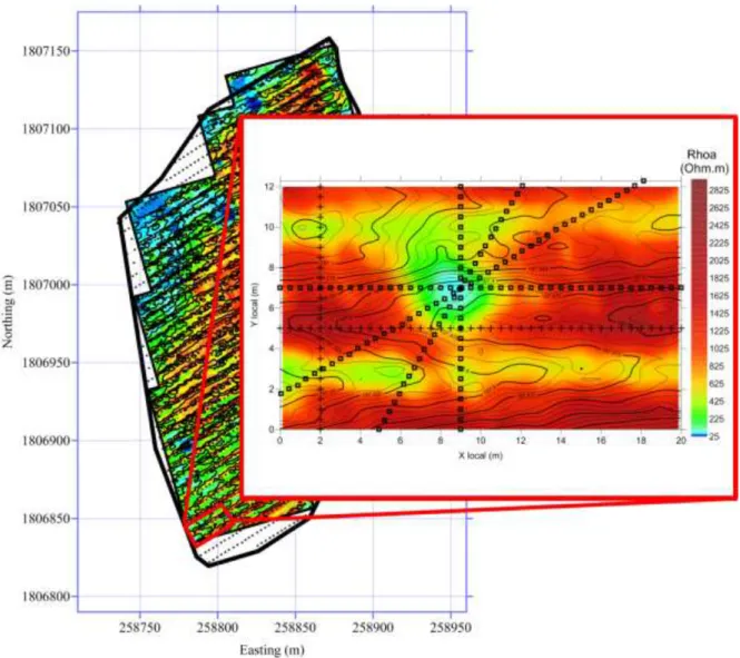
In order to better identify the sources of the anomalies observed on the electrical resistivity mapping, a relatively small area (20 m x 12 m) was selected in the southwest of the BNT 2 site to conduct more detailed surveys (Figure 9). This area, centered on a rank of trees, includes both extended resistant anomalies and a conductive anomaly on the topographic structure.

To simplify their representation, maps are all referenced in a local coordinate system associated with this small study area. In this system, the x-axis is parallel to the trees rank and oriented in the direction SW-NE while the y-axis has a SE-NW orientation.

13

Figure 9 : Location of the detailed study area on the experimental site. On the enlargement of the apparent electrical resistivity map, squares and crosses represent the position of azimuthal profiles.

6.2.1

M

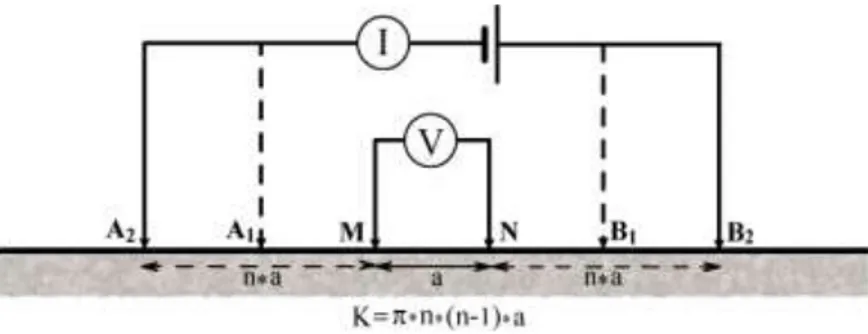
A measurement of apparent electrical resistivity a requires four electrodes: two electrodes (called "current electrodes or A and B") to inject electrical current into the ground with a controlled intensity I, and two other (called "potential electrodes or M and N") to measure the potential difference V created by this current. The apparent electrical resistivity is calculated by a formula, derived from Ohm's law: I V K 



where K is the geometric factor depending on the distances between the 4 electrodes. It is defined by:

;

14

Apparent electrical resistivity mapping in Ban Non Tun was performed using a "pole-pole" electrode array (Figure 10). With this configuration, electrical resistivity mapping is performed by moving only two electrodes (A and M, also called "moving electrodes"), the other two (B and D, also called "fixed electrodes") being installed at a distance of at least 20 to 25 times the maximum distance between the moving electrodes, which is considered infinite because of their small influence on the measurements.

Figure 10 : “Pole-pole” electrode array.

In addition to this array, measurements of apparent electrical resistivity on the small area were performed with electrode configurations "Wenner-α", "Wenner-Schlumberger" and axial "dipole-dipole".

The particularity of the "Wenner-α" device (Figure 11) is to have the same spacing between all the electrodes (AM = MN = NB = a), the potential electrodes M and N being positioned on the same line between the current electrodes A and B.

Figure 11 : “Wenner-α” electrode array.

The "Wenner-Schlumberger" array (Figure 12) is an evolution of the "Wenner-α" device in which the AM and NB distances are equal to n times the distance between the two potential electrodes M and N (also called "measuring dipole").

15

The axial "dipole-dipole" array (Figure 13) is characterized by an identical spacing between the current electrodes A and B and the potential electrodes M and N (MN = AB = a), all being aligned on the same line. The distance between the centers of the two dipoles is a multiple of the size of the dipoles (na).

Figure 13 : Axial “dipole-dipole” electrode array.

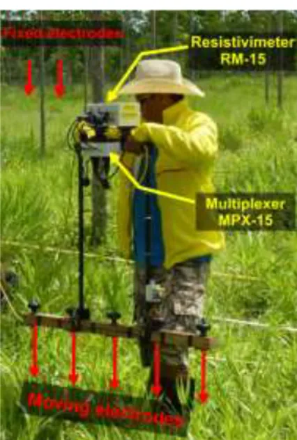
The apparent electrical resistivity measurements were done using a "RM-15" resistivimeter with a "MPX-15" multiplexer (Figure 14) allowing up to eight successive measurements for the same position.

Figure 14 : Resistivimeter “RM-15” and multiplexer “MPX-15”.

To facilitate displacement, the resistance-meter and the multiplexer are fixed on a versatile modular frame whose basis is a beam on which are mounted stainless steel electrodes with a fixed spacing (Figure 15). In order to implement measurements with all the arrays described above, three different beams were used: a 1-m beam with 5 electrodes spaced with 0.25 m, a 2-m beam with 5 electrodes every 0.5 m and a 1.25-m beam with six electrodes separated by 0.25 m.

16

The apparent resistivity measurements are recorded after having created a good contact between the ground and the electrodes. For each position, by using a specific protocol programmed in advance, this device enables to carry out 8 measurements in "pole-pole" array with three different spacing between the electrodes A and M.

The use of the 1-m beam with 5 electrodes allows to perform: • 4 measurements with a = 0.25 m;

• 2 measurements with a = 0.5 m;

• 2 measurements with a = 1 m (by reversing A and M for the second measurement). The same protocol was used with the 2-m beam (5 electrodes), giving the possibility of:

• 4 measurements with a = 0.5 m; • 2 measurements with a = 1 m;

• 2 measurements with a = 2 m (by reversing A and M for the second measurement).

Another protocol enables to complete measurements with the configurations α", "Wenner-Schlumberger" and "dipole-dipole" using the 1.25 m-beam with 6 electrodes:

• 3 "Wenner-α" measurements with a = 0.25 m;

• 1 "Wenner-Schlumberger" measurement with a = 0.25 and n = 3; • 3 "dipole-dipole" measurements with a = 0.25 and n = 1;

• 1 "dipole-dipole" measurements with a = 0.25 and n = 3.

The use of multiple inter-electrode spacing provides apparent electrical resistivity maps integrating different depths. For a homogeneous medium, we consider that the investigation depth corresponds to:

• the distance between A and M for the "pole-pole" array;

• half the distance between the centers of the two dipoles for the "dipole-dipole" array; • AB / 3 for "Wenner-α";

• AB / 2 for "Wenner-Schlumberger".

The literature review allowed us to distinguish the different responses observed on an identical topographical structure when using different electrode arrays [Fox et al., 1980]. It also showed that the topographic effect depends on the electrodes orientation and the prospection direction compared to the axis of the structure.

To use these features, very detailed mapping of apparent electrical resistivity was carried out on the small experimental area using the four devices described above. For each device, a double mapping was performed by changing the orientation of the electrodes alignment, and always keeping the direction of profile perpendicular to the axis of the topographic structure. The resolution of these maps becomes higher for small electrode spacing (from 2 m x 2 m for a = 2 m to 0.25 x 0.5 m for a = 0.25 m).

17

6.2.2 P

6.2.2.1 COMPARISON OF MAPS OBTAINED WITH DIFFERENT ELECTRODE ARRAYS

The results of apparent electrical resistivity mapping obtained on the small surface by "pole-pole", "Wenner-α" and "dipole-dipole" arrays with the same inter-electrode spacing 0.25 m were compared to study the probable differences between responses observed on the same structures (Figure 16). The observation protocols selected for surveys with the "pole-pole" array allow to obtain a homogeneous and equidistant distribution of measurement points using the beams with 5 electrodes (Figure 16.a.). For "Wenner-α" (Figure 16.b.) and" dipole-dipole" (Figure 16.c.) arrays, we use the beam with six electrodes. The measurement points distributions are then heterogeneous (lack of points between profiles) and the positions of the measurements are not identical for the maps made with these different devices. These differences in measurement point density and positioning can cause difficulties to compare maps. To overcome these difficulties, we applied the nearest neighbor interpolation method with a regular sampling identical for all maps. The same color scale is used to represent values of apparent electrical resistivity.

On the three maps, we can distinguish a highly conductive anomaly with a circular shape of diameter 5 to 6 m and coordinates of center: x = 9 m and y = 7 m. The highly resistant and extended anomaly, corresponding to the tree rank, is limited by two slightly conductive anomalies that extend into the inter-rank areas. We can also notice two resistant anomalies near the upper and lower limits of the map corresponding to the two ranks of trees adjacent to the study area.

Comparison of these maps shows that the conductive circular anomaly is wider on the "pole-pole" map than on the two other maps. The minimum observed value of resistivity at the center of this anomaly is 70 Ohm.m for the "pole-pole" map, while on the other two maps this area is characterized by values of about 100 Ohm.m. We can also notice that the geometric dimensions of the anomalies corresponding to the inter-ranks are bigger on the "pole-pole" map, with lower electrical resistivity values compared to the other two maps. The resistant anomaly corresponding to the elevated structure shows maximum values of electrical resistivity higher on the "Wenner-α" and "dipole-dipole" maps (2700 and 2900 respectively Ohm.m) than on the "pole-pole" map (2200 Ohm.m). All features of these anomalies enable to assume that the investigation depth of the "pole-pole" array is higher than the other two.

The raised portions of relief corresponding to the ranks of trees were established by extracting soil in the inter-ranks areas to transfer it on the lines of tree. This has certainly led to a significant deterioration of the structure of these soils, which could result in an increase in their electrical resistivity. By taking into account the better characterization of this resistant superficial layer by "Wenner-α" and "dipole-dipole" arrays (with a spacing of 0.25 m), we can assume that its thickness is very limited, probably less than 20 cm (Figure 16).

Figure 16 : Maps of apparent electrical resistivity for three arrays (a. "pole-pole" with a = 0.25 m; b. "Wenner-α" with a = 0.25 m; c. "dipole-dipole" with a = 0.25 m and n = 1). The black dots represent the positions of the measurements.

19

6.2.2.2 COMPARISON OF MAPS OBTAINED WITH THE “POLE-POLE” ARRAY FOR SEVERAL ELECTRODE SPACINGS

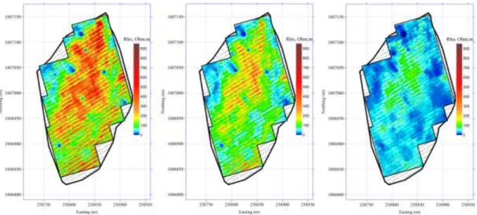
The mapping performed using the "pole-pole" array with different spacings between the moving electrodes (a = 0.25, 0.5, 1 and 2 m) provides information on the distribution of electrical resistivity at different depths. The comparison of these maps shows a considerable decrease of ρa values with increasing depth (Figure 17).

For depths corresponding to electrode spacing 0.25 m (Figure 17.a.) and 0.5 m (Figure 17.b.), the circular conductive anomaly is clearly visible in contrast with the resistant background of superficial layers. On the map obtained with an electrode spacing of 1 m (Figure 17.c.), we observe a general decrease of ρa values and a trend to their homogeneous distribution. On this map, we can still distinguish residue of highly resistant parts corresponding to the superficial layers and the central part of the circular anomaly. To a depth corresponding to an electrode spacing of 2 m (Figure 17.d.), we can only distinguish its shape in the resistant background corresponding to the rank of trees. The existence of a clay layer in the alteration zone at the interface with the bedrock could explain the important decrease of electrical resistivity values observed at this depth.

The anomaly corresponding to the rank of trees is visible on all maps. The intensity of this anomaly decreases when increasing electrode spacing (2000 Ohm.m for a = 0.25 m, 1200 Ohm.m for a = 0.5 m, 500 Ohm.m for a = 1 m and 80 Ohm.m for a = 2 m). We can notice a significant decrease of its width by comparing the maps corresponding to electrode spacing 0.5 and 1 m.

Anomalies corresponding to inter-ranks areas become slightly more conductive between electrode spacings 0.25 and 0.5 m (from 500 to 300 Ohm.m) and their width increases from about 1 to 2 m. On the map obtained with an electrode spacing of 1 m, these anomalies can no longer be distinguished in the background of conductive layers present at this depth. On the map produced with an electrode spacing of 2 m, we can see two extended and highly conductive anomalies. These anomalies are slightly shifted from the positions of the anomalies corresponding to inter-ranks on maps obtained with smaller electrode spacing.

Figure 17 : Electrical resistivity maps obtained with a "pole-pole" array for different electrode spacings (a = 0.25 a. m, b. a = 0.5 m, c. a = 1 m, d = 2 m).

21

We used results obtained in both profile directions with pole-pole configuration for an inter-electrode spacing of 25 cm to calculate the index of anisotropy in the horizontal plane (Figure 18). Results of several studies show that the influence of topography on electrical resistivity measurements depends on the alignment of the electrodes in relation to the structure. It would therefore be natural, in the presence of a topographic effect, to wait for evidence of high anisotropy in the area corresponding to the topographic structure.

Figure 18 : Anisotropy in the horizontal plane and contour lines of electrical resistivity (a.) and topography (b.).

Index values of anisotropy are on average very close to 1, except for some isolated points located in areas characterized by high gradients of the electrical resistivity, which can be observed by overlaying the contours of ρa on this map (Figure 18.a). We do not observe the same consistency with topographic contour lines (Figure 18.b).

We can see that the area corresponding to the topographic structure is characterized by index values close to 1. This result confirms that the topographical effect is very small compared to the influence of the superficial resistant layer. The high values of the index are probably related to the electrode position uncertainty.

During the mapping with the "pole-pole" array, measurements with electrode spacing of 0.5 m (Figure 19) and 1 m (Figure 20) were performed twice successively using the 1-m beam (Figure 19.a and Figure 20.a) and the 2-m beam (Figure 19.b and Figure 20.b). As all measurements were performed on the same points, we can make a comparison between the two maps to assess the reproducibility of measurements and estimate the uncertainties that may be caused by a difference in electrode positioning. For this purpose, the differences between values of ρa observed on both maps were calculated and expressed as a percentage (Figure 19.c and Figure 20.c).

A visual comparison between the two maps obtained for the same inter-electrode spacing does not reveal any particularly noticeable differences. The representation of the differences between the values corresponding to the same spacing and at the same measurement point shows uncertainties under ± 18 % for a spacing a = 0.5 m and less than ± 15 % for a spacing a = 1 m.

22

Figure 19 : Maps of apparent electrical resistivity with the "pole-pole" array for an electrode spacing of 0.5 m (a. map obtained with the 1-m beam, b. map obtained with the 2-m beam, c. uncertainty values overlaid with contour lines of apparent electrical resistivity).

The superposition of electrical resistivity contour lines with the distribution of uncertainties shows that the high uncertainty values often correspond to transition zones between the various anomalies, characterized by high resistivity gradients.

A careful analysis of these uncertainties in the boundary zones between resistant and conductive anomalies reveals a slight shift (15-20 cm to the left) of the 2 m beam compared to the 1 m beam during surveys. If we accredit these uncertainties (up to ± 20 % in our case) only to differences in electrode positioning, this can result in a maximum shift of 15-20 cm of the anomaly limits on the map obtained using the 2 m beam. Such an error is acceptable for soil mapping covering areas of several hectares.

23

Figure 20 : Maps of apparent electrical resistivity with the "pole-pole" array for an electrode spacing of 1 m (a. map obtained with the 1-m bea1-m, b. 1-map obtained with the 2-bea1-m, c. uncertainty values overlaid with contour lines of apparent electrical resistivity).

6.3 S

:

The theory of electrical prospecting is based on the assumption of a tabular or homogeneous environment with a flat surface. In real conditions, the topographic structures may have an influence on the apparent electrical resistivity measurements.

Numerical calculations of anomalies caused by bodies of different geometries began in the late 60's by first using integral equations [Dieter et al., 1969], finite element [Coggon, 1971] and finite difference methods [Mufti, 1976] in two dimensions. 3D calculations by finite differences have also been made [Dey and Morrison, 1979] but this approach requires an orthogonal grid and is not suitable for modeling complex structures. The first scientific works were aimed to find analytical solutions taking into account the influence of topography on ρa measurements.

In one of the first papers, the authors represented the topography as a dihedron in a homogeneous medium or with layers separated by inclined planes to the surface [Cecchini and Rocroi, 1980]. They present the results of calculations made for electrical soundings with Schlumberger array under different azimuths relative to the axis of the topographic structures in a homogeneous medium (100 Ohm.m). The authors show that a topographical structure (horizontal part followed by an inclined portion of 20 ° down or up) can significantly change the survey diagrams. A hasty interpretation of

24

these curves could suggest the presence of two or three layers according to the inclination of the slope and orientation of the device.

For a two-layer medium (50 and 200 Ohm.m) forming a bevel at the foot of a hill, survey curves can be interpreted as the response of a medium with 3 or 4 layers depending on the direction of the device. Several Schlumberger acquisitions were also modeled for profiles perpendicular to the axis of the topographic structure (hill and valley). For a homogeneous medium, the resistivity values observed in these profiles decrease from 20 to 40% for a positioning of the device at the top of the hill and increase from 20 to 50% for the positions of the device corresponding to the bottom of the valley.

In another scientific work, the authors present the results of a study of anomalies generated by topographic structures during electrical resistivity tomography with a dipole-dipole array [Fox et al., 1980]. They used a 2D finite element code to model three simple topographic structures (hill, valley and slope). In calculations using the finite element method, the medium is represented by a mesh of triangular elements. In each element, the unknown potential can be expressed by a simple linear function. This function is defined by the unknown potential of the three vertices of the element, the coordinates of these vertices and the electrical properties of the element. The topographic surface is defined by assigning a very high resistivity value (105 Ohm.m) to the portion of the model corresponding to the air. The electrodes are placed at the air-ground interface with an equidistant spacing which is defined either horizontally or along the slope. This approach was validated by a conclusive comparison of numerical results with the values measured on a physical model presented in [Hallof, 1970].

Fox et al., 1980 made their calculations on a homogeneous model by changing different parameters

(slope length and angle, electrode positions) of the studied topographic structures. They showed that when using a dipole-dipole array, a valley produces a conductive anomaly in the center and two low resistant anomalies at the edges. Under the same conditions, a hill generates an opposite effect - resistant anomaly centered at the top and low conductive anomalies at the edges. In both cases, the topographic effect increases at the start (n = 3 ÷ 4) and decreases (n> 5) with increasing the distance between the two dipoles. For a structure representing two horizontal surfaces of different altitudes connected by a slope, we obtain a conductive anomaly when the injection dipole is located on the slope and the measuring dipole on the lower horizontal part. They observed a resistant anomaly when the measuring dipole is on the upper horizontal part. They also showed that the electrical resistivity anomalies generated by topographic effects are significant for slopes over 10° whose lengths exceed several times the spacing of the dipole.

To complement the work of Fox et al., 1980, a study of the topographic effect in 2D was performed on several topographic structures (vertical wall, hill, valley and slope) with different measuring arrays (pole-pole, dipole-dipole, Wenner-α, pole-dipole) [Tsourlos et al., 1999]. Pole-pole and dipole-dipole arrays produce anomalies similar with a hill (resistant at the top, conductive at the edges with a more marked contrast with the dipole-dipole). A valley produces an opposite effect to that observed for a hill. When using a Wenner-α array, the same structures generate topographic anomalies with opposite forms and less contrasted than with the dipole-dipole array.

In recent scientific papers, we can find more results on the development of techniques for performing three-dimensional numerical calculations. The use of an unstructured tetrahedral mesh

25

allows to refine the mesh near the electrodes, which reduces calculation errors. Indeed, it is necessary to use a mesh as fine as possible in the area around the electrodes where the potential gradients are the highest [Rücker et al., 2006]. This type of mesh also has the advantage of being able to model all types of topographic and geological structures, unlike hexahedral meshes used by many authors [Holcombe and Jiraseck, 1984; Sasaki, 1994; Yi et al., 2001].

This new 3D finite element approach using an unstructured tetrahedral mesh also helped to develop new codes of 3D inversion [Günther et al., 2006] that incorporate topography in the models.

Analysis of these works concerning the modeling and the evaluation of the topographic effect shows the advantages of the modeling method described by Rücker et al. (2006). This method appears to be the most appropriate for simulating the topographic effect. The literature review provided us a quantitative estimate of the topographic effect on measurements of apparent electrical resistivity. However, it is difficult to apply to our results the approaches and methods proposed for the correction of this effect, due to a very complex distribution of electrical resistivity and topographic irregularities. It is therefore important to perform numerical calculations in order to develop a specific approach to correct the results obtained in Ban Non Tun.

6.4 T

Numerical calculations were performed using the software COMSOL Multiphysics. One of its features is the possibility to inject electrical current from a single source point. This considerably simplifies models for calculating resistivity values with "pole-pole" electrode array. COMSOL uses the finite element method (1D to 3D) with an unstructured tetrahedral mesh to model relatively complex topographical structures [Rücker et al., 2006].

We began calculation on a simple homogeneous parallelepipedic model with an electrical resistivity of 1000 Ohm.m and dimensions 100 x 100 x 50 m (Figure 21). It is crossed in the direction of its width by a 4 m wide and 0.5 high topographic structure. The axis of this structure is located at the center of the model length.

The air-ground interface of the model is characterized by a condition of electrical insulation n.J = 0. We assign a potential V = 0 to the deep edges of the model ("Ground" boundary condition). Electrodes are located at the surface in the center of the model in order to minimize boundary effects associated to these conditions.

The area surrounding electrodes is characterized by high potential gradients. It is therefore imperative to use a fine enough mesh around them to precisely define potential values. To refine the mesh only in this area, we use a subdomain with reduced dimensions around the electrodes. We can thus generate mesh with element size less than 1 / 5 of the minimum distance between electrodes. In order to reduce calculation time, a coarser mesh is used in the rest of the model, where the potential gradients are low,

Calculations were performed for 25 positions of a five-electrode device, spaced every 0.5 m and aligned parallel (00° orientation) and perpendicular (90° orientation) to the topographic structure axe. The device is moved along a profile perpendicular to the structure with a step of 0.5 m between two positions. This allows the simulation of resistivity values corresponding to the profiles made on

26

the site with RM15 in "pole-pole" electrode configuration for inter-electrode spacing: a = 0.5 m, a = 1 m and 2 = m.

The association of COMSOL and MATLAB softwares allows to calculate and to store potential values at points corresponding to the position of measuring electrodes for each position of the injection electrode. The apparent resistivity is then defined using the calculated values of potential V, the intensity of injected current (I = 100 mA) and geometric coefficients of the devices (K = 2πa).

Figure 21 : Homogeneous model with a resistivity of 1000 Ohm.m used for simulations of topographic effect.

Results for both orientations of the device show clearly a resistant anomaly corresponding to the top of the topographic structure (Figure 22). We can observe low resistivity anomalies on both edges of the topographic structure (hereafter called “lateral anomalies”). Apparent electrical resistivity values calculated for the flat part of the model correspond to the electrical resistivity of the model (1000 Ohm.m) with an error less than 5 % for the three inter-electrode spacing (990 Ohm.m for a = 0.5 m , 980 Ohm.m for a = 1 m and 960 Ohm.m for a = 2 m).

Amplitudes of the anomalies calculated with the 00° orientation (Figure 22.a.) are very close for the apparent electrical resistivity calculated with the three inter-electrode spacing (about 10 % of the resistivity calculated on the flat part for the central resistant anomaly and 5 % for the lateral anomalies). Amplitudes of resistant anomalies are higher with the 90° orientation (Figure 22.b.), and increase with inter-electrode spacing (12 % for a = 0.5 m, 18 % for a = 1 m and 22 % for a = 2 m). Inversely, amplitudes of the lateral anomalies decrease with inter-electrode spacing (14 % for a = 0.5 m, 13 % for a = 1 m and 11 % for a = 2 m).

27

Figure 22 : Apparent electrical resistivity calculated on a homogeneous model with three electrode spacing.

The topographic structure has a clear influence on the calculated electrical resistivity values, but these anomalies are lower (around 1100 Ohm.m) than those observed on the field (up to 1400 Ohm.m for a = 0.5 m).

According to ERT results, a 1-m thick resistive layer (around 1000 Ohm.m) lays on top of a conductive substratum (around 100 Ohm.m). Results of detailed electrical resistivity mapping have also shown the presence of a superficial resistant layer in the topographic structure (probably around 3000 Ohm.m). Therefore, we used a 3-layer model corresponding to those features in order to obtain amplitudes of anomalies similar to those observed on the site (Figure 23).

28

The apparent electrical resistivity calculated with a 3-layer model show clear resistive anomalies corresponding to the topographic structure in both orientations of the device (Figure 24). The lateral anomalies are only visible with the 90° orientation. The presence of the deep conductive layer generates a differentiation of resistivity values corresponding to the plane part of the model.

The electrical resistivity values calculated on the top of the topographic structure (around 1800 Ohm.m for a = 0.5 m) are higher than those observed on the site (around 1400 Ohm.m for the same electrode spacing). Values calculated for the plane part of the model are also too high (around 700 Ohm.m for a = 0.5 m) compared with the values measured in the inter-rank areas of the site (around 400 Ohm.m for the same electrode spacing). It confirms the presence of a superficial resistant layer on the rank of trees, with probably a more conductive deep layer (around 20 Ohm.m).

29

7 C

ONCLUSIONS

The results obtained during my internship allow the following conclusions:

 results of geophysical mapping shows that anomalies of different geophysical parameters reflect soil spatial variability;

 comparison of electrical resistivity and topographic maps revealed a significant coherence between the topographic structures corresponding to the ranks of trees and the extended resistant anomalies;

 results of numerical modeling show that electrical resistivity values can be influenced by topographic structure, with amplitudes lower than those observed on the “Ban Non Tun” site;

 comparison of calculated results with detailed electrical resistivity mapping performed with several electrode configurations allowed us to show the existence of a superficial resistant layer on the rank of trees, probably of anthropogenic origin.

8 R

ECOMMENDATIONS

Previous results obtained in the NRCT project "Use of Electrical Resistivity and Self Potential Mapping for Sustainable Agriculture: Application to Rubber Tree Plantations in North-East Thailand” and the new results provided by my internship show the effectiveness of geophysical parameters to characterize soils variability and their evolution.

Thus, the use of applied geophysical methods is recommended in the different phases of soil studies, from the pre-inspection to characterize the site and fix the boundaries of the experimentation, to the monitoring of the soil spatiotemporal evolution during the survey.

30

9 R

EFERENCES

Cecchini, A., and J. P. Rocroi (1980), Effet topographique en prospection électrique, Geophysical

Prospecting, 28(6), 977-993.

Coggon, J. H. (1971), Electromagnetic and electrical modeling by the finite element method,

Geophysics, 36(1), 132-155.

Dey, A., and H. F. Morrison (1979), Resistivity modeling for arbitrarily shaped three-dimensional structures, Geophysics, 44(4), 753.

Dieter, K., Paterson, N.R., and Grant, F.S. (1969), IP and resistivity type curves for three-dimensional structures, Geophysics, 34, 615-632.

Fox, R. C., G. W. Hohman, T. J. Killpack, and L. Rijo (1980), Topographic effects in resistivity and induced-polarization surveys, Geophysics, 45(1), 75.

Gonçalves, P. de S., A. K. Fujihara, A. A. Ortolani, O. C. Bataglia, N. Bortoletto, and I. Segnini Junior (1999), Phenotypic stability and genetic gains in six-year girth growth of Hevea clones, Pesquisa

Agropecuaria Brasileira, 34, 1223 - 1232.

Günther, T., C. Rücker, and K. Spitzer (2006), Three‐dimensional modelling and inversion of dc resistivity data incorporating topography – II. Inversion, Geophysical Journal International, 166(2), 506-517.

Hallof, P. G. (1970), Theoretical induced polarization and resistivity studies, scale model cases, phase III, McPhar Geophysics Ltd.

Holcombe, H. T., and G. R. Jiraseck (1984), Three-dimensional terrain corrections in resistivity surveys, Geophysics, 49(4), 439.

Hovhannissian, G. M., J.-P. Pozzi, P. Bernard, and A. Tabbagh (2002), Transient electric phenomena observed during fluid circulation in unsaturated porous media, Geophys. Res. Lett., 29, 4 PP.

Moeys, J., B. Nicoullaud, A. Dorigny, Y. Coquet, and I. Cousin (2006), Cartographie des sols à grande échelle : integration explicite d’une mesure de résistivité apparente spatialisée à l’expertise pédologique, Etude et gestion des sols, 13(4), 269-286.

Mufti, I. R. (1976), Finite-difference resistivity modeling for arbitrarily shaped two-dimensional structures., Geophysics, 41(1), 62.

Pinettes, P., P. Bernard, F. Cornet, G. Hovhannissian, L. Jouniaux, J.-P. Pozzi, and V. Barthés (2002), On the Difficulty of Detecting Streaming Potentials Generated at Depth, Pure and Applied

Geophysics, 159(11-12), 2629-2657.

Rao, P. S., C. K. Saraswathyamma, and M. R. Sethuraj (1998), Studies on the relationship between yield and meteorological parameters of para rubber tree (Hevea brasiliensis), Agricultural and Forest

Meteorology, 90(3), 235-245.

Rücker, C., T. Günther, and K. Spitzer (2006), Three‐dimensional modelling and inversion of dc resistivity data incorporating topography – I. Modelling, Geophysical Journal International, 166(2), 495-505.

Samouëlian, A., I. Cousin, A. Tabbagh, A. Bruand, and G. Richard (2005), Electrical resistivity survey in soil science: a review, Soil and Tillage Research, 83(2), 173-193.

Sasaki, Y. (1994), 3-D resistivity inversion using the finite-element method, Geophysics, 59(12), 1839. Tabbagh, A., M. Dabas, A. Hesse, and C. Panissod (2000), Soil resistivity: a non-invasive tool to map soil structure horizonation, Geoderma, 97(3-4), 393-404.

Telford, W. M., L. P. Geldart, and R. E. Sheriff (1990), Applied Geophysics, 2nd ed., Cambridge University Press.

Tsourlos, P. I., J. E. Szymanski, and G. N. Tsokas (1999), The effect of terrain topography on commonly used resistivity arrays, Geophysics, 64(5), 1357.

Watanabe, K., T. Yamamoto, T. Yamada, T. Sakuratani, E. Nawata, C. Noichana, A. Sributta, and H. Higuchi (2004), Changes in seasonal evapotranspiration, soil water content, and crop coefficients in sugarcane, cassava, and maize fields in Northeast Thailand, Agricultural Water Management, 67(2), 133-143.

Williamson D.R., Peck A.J., Turner J.V., and Arunin S. (1989), Groundwater hydrology and salinity in a valley in Northeast Thailand, Groundwater contamination. IAHS Publ., 185: 147-154.

Yi, M., J. Kim, Y. Song, S. Cho, S. Chung, and J. Suh (2001), Three‐dimensional imaging of subsurface structures using resistivity data, Geophysical Prospecting, 49(4), 483-497.