HAL Id: hal-01111782
https://hal.archives-ouvertes.fr/hal-01111782v2
Submitted on 13 Oct 2018
HAL is a multi-disciplinary open access archive for the deposit and dissemination of sci-entific research documents, whether they are pub-lished or not. The documents may come from teaching and research institutions in France or
L’archive ouverte pluridisciplinaire HAL, est destinée au dépôt et à la diffusion de documents scientifiques de niveau recherche, publiés ou non, émanant des établissements d’enseignement et de recherche français ou étrangers, des laboratoires
Investigating soundscapes perception through acoustic
scenes simulation
Grégoire Lafay, Mathias Rossignol, Nicolas Misdariis, Mathieu Lagrange,
Jean-François Petiot
To cite this version:
Grégoire Lafay, Mathias Rossignol, Nicolas Misdariis, Mathieu Lagrange, Jean-François Petiot. In-vestigating soundscapes perception through acoustic scenes simulation. Behavior Research Methods, Psychonomic Society, Inc, 2019, 51 (2), pp.532-555. �hal-01111782v2�
Investigating soundscapes perception through acoustic
scenes simulation
G. Lafay1), M. Rossignol2), N. Misdariis2), M. Lagrange1), J-F. Petiot1)
1)Laboratoire des Sciences du Num´erique de Nantes-CNRS- ´Ecole Centrale de Nantes,
Nantes, France. [email protected]
2) STMS Ircam-CNRS-SU Institut de Recherche et Coordination Acoustique/Musique,
Paris, France
Abstract
This paper introduces a new experimental protocol to study mental repre-sentations of urban soundscapes through a simulation process. Subjects are asked to create a full soundscape by means of a dedicated software tool, cou-pled with a structured sound data set. This paradigm is used to character-ize urban sound environment representations by analyzing the sound classes that were used to simulate the auditory scenes. A rating experiment of the soundscape pleasantness using a 7-point bipolar semantic scale is conducted to further refine the analysis of the simulated urban acoustic scenes. Results show that 1) a semantic characterization in terms of presence / absence of sound sources is an effective way to characterize urban soundscapes pleas-antness, and 2) acoustic pressure levels computed for specific sound sources better characterize the appraisal than the acoustic pressure level computed over the overall soundscape.
Keywords: cognitive psychology, soundscape perception, soundscape simulator
1. Introduction
One of the main goals of soundscape studies is to identify which compo-nents of the soundscape influence human perception, see Aletta et al. (2016). Establishing a link between an environment (urban sound scene) and the in-duced human sensation (calmness) is equivalent to instantiating the mental
representation of a specific sound scene (a calm urban sound scene). Several means have been considered in the literature to perform this task.
First, a subject can be asked to assess a given sound following a given perceptual scale (e. g. calmness, pleasantness), see Axelsson et al. (2005); Davies et al. (2013); Cain et al. (2013). The amount of information that can be gathered strongly depends on the nature of the available stimuli, be they recorded sound scenes as part of a within laboratory experiment, or in situ. Working with actual stimuli makes it possible to analyze them, thus allowing the experimenter to gather a coarse-grained physical description of them.
Second, a subject can be asked to describe a given sound environment, see Guastavino (2006); Dubois et al. (2006). A large amount of quantitative and semantic information is then collected about the subject’s representation of this type of sound environment. Unfortunately, without any reference to sound data, this representation can hardly be characterized physically.
We propose in this paper to consider the use of a soundscape simulator that the subject can employ to objectify his/her representation of a given sound environment. We believe that the use of such a device allows us to gain the benefits of the two above mentioned approaches. As the subject is asked to produce audio data (the signal of the simulated scene), it allows the experimenter to study a precise modal version of the subject’s mental representation that is characterized both semantically (the nature of sound sources) and physically (e. g. the levels of sound sources).
We believe that the availability of a fine grain description of the sound stimuli is of great interest, because recent studies demonstrate that all sound sources do not contribute equally to the perception of the sound scene, see Defr´eville et al. (2004); Lavandier & Defr´eville (2006); Guastavino (2006); Nilsson (2007); Szeremeta & Zannin (2009). Thus, much attention is given to the specific contributions of the different sources to the notion of emotional quality of the scene, see Gozalo et al. (2015); Ricciardi et al. (2015).
For several reasons that are detailed in this paper, the use of a sound-scape simulator such as the one proposed here can lead to interesting out-comes as it allows the experimenter to separately study the influence of the sound sources that compose a sound environment. With such material, not only is the type of sound sources available for study, but also the exact sound level and audio waveform for each source together with the structural prop-erties of the scene, that is, the temporal distribution of the sound events.
To demonstrate the potential of the proposed approach in its ability to question the human perception of sound environments, we study in this
paper the notion of perceptual pleasantness of urban environmental scenes. Results and outcomes of a series of three experiments that build upon the use of the simulator are studied in order to better comprehend how different sound sources typically present in a urban scene impact pleasantness:
1. experiment 1.a, simulation: the subjects use the soundscape simulator to produce ideal / non-ideal soundscapes that are considered as mate-rial for the following experiments (the resulting waveforms are available for download1);
2. experiment 1.b, pleasantness evaluation: the subjects judge the pleas-antness of the simulated scenes on a semantic scale;
3. experiment 2, pleasantness evaluation after modification of the scenes: the subjects judge the pleasantness of the simulated scenes on a seman-tic scale as in 1.b, but some scenes are modified beforehand, i. e. some specific sounds classes that are identified as having a significant impact on perceived pleasantness are removed.
To the best of our knowledge, only Bruce et al. (2009); Bruce & Davies (2014) considered the use of a simulator to question soundscape perception. They propose a tool that allows the user to modify a given soundscape by adding or removing specific sound sources, by changing the acoustic level of the sources as well as their spatial location. The authors show that the addition or removal of the sources globally follows social or semantic con-siderations more than their acoustical characteristics. A lack of diversity in terms of sound sources is nonetheless mentioned by the authors as a limiting factor to the strength of the outcomes given in this study.
In our approach, the simulator developed for this study2 only yields a monophonic representation of the scene, but that simplification comes with the benefit of a wider range of available sound sources and scheduling pa-rameters in order to provide outputs which are both expressive and useful for analysis.
The remaining of this paper is organized as follows: the soundscape sim-ulator simScene is introduced in Section 2. Experiments 1.a simulation and 1.b pleasantness evaluation are presented in Section 3. Experiment 2 pleas-antness evaluation after modification of the scenes is presented in Section 4. Conclusions and discussion about future work follow in Section 5.
1Soundscapes: https://archive.org/details/soundSimulatedUrbanScene
2. The simulator
Simscene is an online digital audio tool whose first version has been developed as part of the HOULE project3. It has been designed to run on the popular
web browsers Chrome and Firefox. It is fully written in javascript using the angular.js library4 and the Web Audio standard that allows the manipulation of digital audio data within the browser5. The interface for selecting sound
sources (cf. Section 2.3) uses the popular D3.js visualization library proposed by Bostock et al. (2011).
Simscene is designed as a simplified audio sequencer, with sequencing parameters specifically chosen for the generation of realistic soundscapes. To do so, the user first selects a sound source using a non verbal selection inter-face presented in Section 2.3. A track is then created for this sound source within the simulator interface. The user can then manipulate some param-eters detailed in Section 2.2 to control the time and magnitude distribution of the occurrences of the sound sources. Text fields are also available for the user to 1) name each track, 2) name the entire scene, 3) provide free comments about the simulated scene.
2.1. Sound database
In order to provide the user with a sound database that is well organized and covers as much as possible the variety of sound sources that are present in urban areas, a typology of urban sounds is first defined.
Typology
The chosen typology is established based on the category/classes of sounds found while reviewing several articles or thesis manuscripts that study how humans discriminate different kind of urban soundscape, see Leobon (1986); Maffiolo (1999); Raimbault (2002); Guastavino (2003); Defr´eville et al. (2004); Beaumont et al. (2004); Raimbault & Dubois (2005); Dubois et al. (2006); De-vergie (2006); Guastavino (2006); Polack et al. (2008); Niessen et al. (2010); Brown et al. (2011) .
3HOULE project : houle.ircam.fr
4angular.js: angularjs.org
We choose not to include any musical content in the sound database, as the study of the pleasantness of a given style or genre of music is beyond the scope of this study.
Events and Textures
A commonly accepted distinction consists in separating:
• sound events: isolated sounds, precisely located in time, whose acous-tical characteristics may change with respect to time;
• sound textures: isolated sounds of long duration whose acoustical char-acteristics are stable with respect to time, see Saint-Arnaud (1995). It indeed appears that the processing of auditory information comprises some sort of decision concerning the nature of the stimuli.
Maffiolo (1999) distinguishes two separated categorization processes, ei-ther of which is triggered depending on the listener’s ability to identify sound events. She shows that those processes lead to two abstract cognitive cat-egories respectively termed ”event sequences” and ”amorphous sequences”. Event sequences are composed of salient events that can easily be recognized, such as car start or male speech. They arise from a descriptive analysis based on the identification of the sound sources. On the contrary, amorphous se-quences are sound environments where distinct events cannot be readily iden-tified, such as traffic hubhub. They result from a holistic analysis based on global acoustic features.
Concerning sound textures, i. e. sounds that have stable characteris-tics over time, McDermott & Simoncelli (2011); McDermott et al. (2013) demonstrates that the human brain can opt for an abstract, statistical repre-sentation of the perceived information, discarding precise physical properties of the sound.
In order to account for the possibility that the morphological differences between sound events and sound textures may have some important conse-quences on the perception of the scenes, the simulation tool Simscene follows this distinction and considers two distinct sound databases: one with classes of events only and the other with classes of textures only. These two types of sound classes also have specific scheduling procedures during the simulation process.
We consider in this study the soundscape as a “ skeleton of events on a bed of textures ” as coined by Nelken & de Cheveign´e (2013).
Sample 1 Sample 2 . . . . Sample n Motorized transport Level 0
(high abstrac1on level) Level 1 (low abstrac1on level)Level 2 Samples
Car
Motorcycle Car start
Car passing by
Figure 1: Hierarchical organisation of the isolated sounds used in the simulation.
Taxonomy
We call “ sample ” a recording of an isolated sound, be it an event or a texture. Each sound class is implemented as a collection of samples judged to be perceptually equivalent.
The sound classes are organized hierarchically (cf. Figure 1) according to a structure similar to the vertical axis of the categorical organization proposed by Rosch & Lloyd (1978). The lower the level of abstraction, the more precise the description of the class and the more perceptually similar the sound sources. For classes with a high level of abstraction that have sub classes, their collection of samples is the union of the collections of the sub classes.
Accounting for the previously detailed perceptual matters, two tax-onomies are built, one for sound events and one for sound textures. Up to four levels of abstraction are considered from the most generic classes (level 0) to the most specific classes (level 3), leading to a taxonomy close to
the one used in Salamon et al. (2014), see Appendix A. Only three levels of abstraction are considered for the texture sounds, see Figure A.11.
Sound samples collection
483 isolated sounds are collected and organized with the two typologies dis-cussed above, 381 events and 102 textures. Among those samples, 332 have been recorded and 151 have been taken from two sound libraries: SoundIdeas6
and Universal SoundBank7.
Original sounds have been recorded using a shotgun microphone AT80358 plugged to a ZOOM H4n9 recorder. The use of such a microphone allowed us
to isolate as much as possible sound events of interest from the urban back-ground. It also allowed us to avoid dominant sound sources while recording texture sounds by targeting distant areas with no dominant sound sources.
All samples are normalized to the same RM S level of −12 dB FS, i. e. relative to Full Scale. In our case, the full scale level is set arbitrarily to 1 Volt.
2.2. Parameters
By a deliberate design choice, the simulation tool does not allow the user to interact with and control directly a specific sample. Interaction is done at the track level, a track being a sequence of samples. Several parameters are available to the subject to control the track:
• sound level (dB): for each sample, the sound levels are drawn randomly following a normal distribution parameterized by the subject in terms of mean value and variance;
• inter-onset spacing (second): for event tracks only, and for each sound event sample, the inter-onset spacings are drawn randomly following a normal distribution parameterized by the subject in terms of mean value and variance;
6
SoundIdeas: www.sound-ideas.com
7Universal SoundBank : www.universal-soundbank.com
8AT8035 shotgun microphone: eu.audio-technica.com
• start and end time (second): the subject sets the start and end times between which the texture or sequence of repeated events occurs. To improve simulation quality, two parameters are also proposed: • event fades (seconds): for the event tracks only, the subject can set a
fade in / fade out duration applied to each sample;
• global fades (seconds): the subject can set global fade in and fade out durations applied to the entire track.
Texture samples are sequenced without time spacing, therefore the pa-rameters event fade and inter-onset spacing are not available for this kind of track.
2.3. Selection interface
Once the typology and the set of sounds are available, an important design issue is the need for a suitable way to display the sound dataset to the user. Most browsing tools are based on keyword indexing; however, for sensory experiments that study the objectivation of a subject’s mental representa-tions, this may be problematic as the availability of a verbal description of the sound can influence the subject’s choice, and potentially induce biases in the analysis conclusions. For example, a subject may automatically se-lect sounds referenced as belonging to a park environment to build a calm soundscape, rather than focusing on their perception.
Therefore, the selection interface considered in this study is text-free and designed so as to force the user to rely on listening.
Figure 2a shows the interface used for the selection of events. Each circle corresponds to a sound class, with the lowest level of abstraction (leaves) colored in grey. The spatial location of those circles is chosen according to the hierarchical organization of the sound database: sub-classes belonging to the same class are close to each others, and so on until the user reaches the leaf classes, which are directly linked to a collection of samples.
Each of those classes has a representative sound chosen arbitrarily by the authors in order to provide the same sound each time the user clicks on the circle. The subject can browse the database by listening to those prototype sounds. The efficiency of this interface compared to several others designs has been evaluated and the outcomes are discussed by Lafay et al. (2016).
(a) Traffic Truck Truck starting (b)
Figure 2: SimScene graphical interfaces for the selection of sound classes (a) and their sequencing (b).
D A T A A N A L Y S I S
sound sample
databases simulated scenes
Experiment 2 pleasantness evalua+on Experiment 1 scene simula+on
1st group of subjects 2nd group of subjects
Figure 3: Experimental protocol of the simulation experiment (1.a) and pleasantness eval-uation experiment (1.b).
2.4. Simulation interface
As shown on Figure 2b, the simulation interface displays a schematic of the scene under creation. Each track is represented as a horizontal strip with a temporal axis. Each sample of this track is displayed as a rectangle whose height is proportional to the amplitude of the sample. For event tracks, the horizontal spacing between those rectangles is a function of the time delay between their onsets. For texture tracks, a unique rectangle is displayed as this kind of sounds does not allow spacing with silence. As the actual amplitude and spacing values are drawn from random variables, each time the subject changes the value of a parameter, the location and height of the rectangles are updated to reflect the changes in the sequencing of the samples. The subject can listen to the resulting sound scene at any time.
As such, the underlying model of the scene is a sum of sound sources. The simulation interface is more thoroughly described by Rossignol et al. (2015).
3. Experiment 1
3.1. Objective
Experiment 1 aims at using a simulation paradigm to investigate the specific influences of the various sound sources constituting urban soundscapes on
the perceived pleasantness. For that, the first two experiments are planned as follows (cf. Figure 3):
• experiment 1.a (simulation): during this experiment, subjects are asked to create simulated urban sound environments using Simscene (see Sec-tion 2). Each of them has to create two sound environments: one ideal / pleasant, and the other non-ideal / unpleasant.
• experiment 1.b (evaluation): after the simulation phase, only a binary information on the pleasantness property of the respective scenes is available: respectively ideal or non-ideal. Furthermore, this informa-tion is given by the creator of the scene. The second experimental step aims at investigating more deeply and more broadly our knowledge on the pleasantness of the simulated scenes. For that, a second group of subjects is asked to evaluate the pleasantness of each scene produced during (1.a), on a semantic scale. This experiment has two goals:
1. to evaluate more precisely the respective influence of the various sources composing the scenes on the pleasantness (ideal or non-ideal) thanks to a finer quantification of the pleasantness of the scene;
2. to detect the presence of outliers or ambiguous scenes. Indeed, throughout our analyses, the predefined hedonic properties of the scenes (ideal or non-ideal) are used as reference. We thus need to ensure beforehand that no ambiguity exists between extreme cases of ideal and non-ideal scenes, i. e. that the least pleasant ideal scene remains more highly rated on average than the most pleasant non-ideal scene.
The data collected by these two experiments (1.a and 1.b) are analyzed conjointly.
3.2. Planning of Experiment 1.a
The design of this experiment has been validated with a pilot study described by Lafay et al. (2014).
Procedure
The subjects are asked to simulate two urban sound environments of one minute each, following these instructions:
• first simulation: create a plausible urban soundscape which is ideal, according to you (where you would like to live);
• second simulation: create a plausible urban soundscape which is non-ideal, according to you (where you would not like to live);
All the subjects start by designing the ideal environment; they read the second set of instructions at the end of the first experiment. Subjects are completely free of their choices concerning sounds and synthesis parameters. The created sound environments must nevertheless fulfill the two following constraints :
• the listening point of view is that of a fixed listener;
• the soundscape must be realistic, i. e. physically plausible. For instance, subjects are free to insert ten dogs in the soundscape but they cannot insert one dog barking every 10 milliseconds.
These constraints are notified in the instructions; no control is done a priori in the simulation interface.
Each simulation process is decomposed into several steps: 1. Simulation, where the user is asked to:
• select sound classes, • give each of them a name,
• set the parameters of the tracks related to the selected sound classes of sounds, see Section 2.2.
2. Feedback : writing of a free form comment about the composed sound-scape.
In addition, once the two sound scenes are completed, the subjects are invited to:
• give a comment about the ergonomics of the simulation environment; • give a comment about the ergonomics of the selection tool.
Before starting the first simulation, a 20-minute tutorial is given in order to familiarize the subjects with the simulation interface and the sound database. The experiment is planned to last about two hours and a half, including breaks that the subjects are allowed to take.
Apparatus
All the subjects performed the experiment on standard desktop computers with the same hardware and software configurations. The audio files were played in diotic conditions using headphones. During the tutorial, subjects were asked to adjust the sound volume to a comfortable level. Once set, they were not allowed to modify it during the remaining of the experiment.
All the subjects performed the experiment at the same time. They were equally distributed in three identical quiet rooms, and were not allowed to talk to each other during the experiment.
Three experimenters (one in each room) were available during the whole duration of the experiment in order to assist subjects with potential hardware and software issues, and to answer questions.
Subjects
44 students (30 male, 14 female; averaging 21.6 years of age, s.d. of 2.0 years) from Ecole Centrale de Nantes (a french engineering school) performed the experiment. All the subjects had been living in Nantes, France, for at least two years at the time of the experiment and reported normal hearing.
Among the 44 subjects, 40 succeeded, producing in the end 80 simulated sound scenes (40 ideal scenes, 40 non-ideal scenes). The 4 other subjects were excluded from the process due to a lack of understanding of the instructions or failure to respect them, or for exceeding the maximum duration allowed to perform the experiment. The software platform used for the experiment, the parametrization of the software platform for each generated scene, as well as a 2 dimensional projection of the resulting scenes are available online10.
3.3. Planning of experiment 1.b
ProcedureThe subjects evaluate the 80 simulated scenes generated in experiment 1.a. Due to temporal constraints, subjects only assess 30 seconds of the initial 1-minute simulated scenes (from sec. 15 to sec. 45).
The assessment is done with a 7-point bipolar semantic scale going from -3 (non-ideal / unpleasant) to +3 (ideal / pleasant). Before evaluating a scene, the subjects must listen at least to the first 20 seconds of the stimuli. After the evaluation, they are free to continue to the next scene.
For each participant, sound scenes are played in a quasi random order. 5 ideal scenes and 5 non-ideal scenes are first sequenced to allow the subjects to calibrate their scores. These first 10 scenes are played back again at the end of the experiment. Only the last evaluations are taken into account. Each participant evaluates all the sound scenes.
The experiment is planned to last 30 minutes. The subjects do not know anything beforehand about the nature of the sound scenes.
Apparatus
All the subjects performed the experiment on standard desktop computers with the same hardware and software configurations. The audio files were played in diotic conditions by semi-open headphones Beyerdynamic DT 990 Pro. The stimuli were the scenes obtained in experiment 1.a. The output sound level was the same for all the subjects.
All the subjects performed the experiment simultaneously in a quiet environment. They were not allowed to talk to each other during the exper-iment.
An experimenter was available during the whole duration of the exper-iment in order to assist subjects and to answer questions.
Subjects
10 students (8 male, 2 female; averaging 23.1 years of age, s.d. of 1.8 years) from Ecole Centrale de Nantes performed the experiment. All the subjects had been living in Nantes, France, for at least two years at the time of the experiment and reported normal hearing. None of them took part in the previous simulation experiment (experiment 1.a).
Terms Abbreviations
Sound level L
Sound level (events) L(E)
Sound level (textures) L(T )
Average pleasantness (per scene) Ascene
Average pleasantness (per subject) Asubject
Table 1: Abbreviations of features used in the analysis of the experiments.
All the subjects succeeded in doing the experiment.
3.4. Data and statistical analysis
A set of features, upon which the analysis is conducted, is attached to each sound scene. A summary of those features (and the corresponding abbrevia-tions) is presented in Table 1. In order to be consistent with the evaluation of experiment 1.b, features are not computed on the whole duration of the sequences but only on their 30-second reduced version used as stimuli for experiment 1.b (Section 3.3).
For each sound scene, three types of features are considered :
• perceptual features: the perceived pleasantness of the composed scene, assessed on a 7-point bipolar semantic scale. Ascene is the average
pleasantness for each scene, computed as the average of all the scores given by all the subjects to a specific scene. Asubject is the average
pleasantness for each subject, computed as the average of all the scores given by a specific subject to all the scenes. Asubject is computed for
ideal scenes and non-ideal scenes separately. Given the low number of subjects in experiment 1.b, we choose not to normalize the pleasantness scores.
• semantic features: we use a boolean vector S = (x1, x2, . . . , xn) that
indicates the classes of sounds involved in the scene, i. e. the sound classes that are present / absent from the scene. Each boolean x of this vector corresponds to a specific class of sounds: x = 1 if the class is present in the scene, and x = 0 otherwise. The vector dimension (n) depends on the level of abstraction that is considered for the analysis. For instance, for the abstraction level 1, that includes 44 classes of sounds, the dimension is thus 44 (n = 44).
• structural features: while SimScene allows us to access a variety of information about the scene structure (such as the density of events), we only focus in this first study on the sound levels. To figure those out, we draw inspiration from the LAeq measure. In our case, it is a scalar
computed from the signal (in Volt and not in Pascal), and converted in decibels, with a reference of 1 Volt (full scale). The level is obtained by computing the quadratic mean of the signal every second and averaging the results over the total duration of the scene. An A-filtering module processes the data before the quadratic means are computed. We note L, L(E) and L(T ) the computed levels by respectively considering the whole set of samples, only the set of event samples, and only the set of texture samples.
In order to evaluate the specific impact of the various sound sources on the perceived pleasantness, we run the data through the five following significance tests:
• Analysis of perceived pleasantness: the goal is to evaluate whether the perceived pleasantness is in accordance with the pleasantness label given by the creators of the ideal and non-ideal scenes during exper-iment 1.a. To do so, we consider if there exist significant differences between the ideal and non-ideal scenes for Ascene and Asubject. The
significance is evaluated by a two-sample Student test for Ascene and
by a paired-sample Student test for Asubject.
• Analysis of sound levels: the goal is to evaluate whether the sound levels (L, L(E) and L(T )) differ between the ideal and non-ideal scenes. The significance is measured with a two-sample Student test.
• Influence of sound levels on perceived pleasantness: the goal is to eval-uate whether the sound levels (L, L(E) and L(T )) affect the perceived pleasantness. To do so, we consider linear correlations between those features and Ascene. The Pearson correlation coefficient is used for that
purpose.
• Analysis of semantic features: the goal is to evaluate whether specific classes are more frequently used in a given type of environment (ideal or non-ideal). To do so, a V-test is considered, see (Rakotomalala & Morineau, 2008). With c being the total number of classes used to
simulate all the scenes, ck the number of classes used to simulate the
scenes of a given type of environment k (ideal or non-ideal), cj the
number of times a class j has been used to simulate all the scenes, and cjk the number of times a class j has been used to simulate the
scenes of a given type of environment k, the V-test evaluates the null hypothesis that the ratio cjk
c is not significantly different from the ratio cjk
ck. For each class j, and each environment type k, an approximation
of the statistical value Vjk is computed as follows:
Vjk = cjk − ck cj c q ckc−cc−1k cj c(1 − cj c) (1)
If the null hypothesis is rejected, the class j is said to be typical with respect to the type of environnement k. Such typical classes are called sound markers, in reference to the work of Schafer (1993). Testing is done for each class, at each level of abstraction, and separately for texture and event classes.
• Representation space induced by the semantic features: the goal is to determine if a representation space of the scenes solely based on the presence / absence of sound sources allows us to distinguish between the two types of scenes. Denoting as Si the semantic features of scene i,
we compute the distances between all Si vectors. A Hamming distance
is used: considering two n-dimension vectors S1 = (x1,1, x1,2, . . . , x1,n)
and S2 = (x2,1, x2,2, . . . , x2,n), with x ∈ {0, 1}, the Hamming distance
dham measures the proportion of coordinates that differ between the
two vectors. It is defined as follows:
dham(S1, S2) = 1 n n X i=1 (x1,i M x2,i) (2)
whereL is the exclusive-or operator. Two scenes having similar source compositions will be close in such a space. Using the Hamming dis-tance allows us to take into account equally the presence and absence of classes. In order to measure the intrinsic ability of the space to dis-criminate between ideal and non-ideal scenes, we use a ranking metric named the precision at rank k (P @k). The P @k computes the
preci-sion obtained after the k closest items to a given seed item have been found. Formally, for each scene si (considered as seed), we compute
the proportion of sj scenes in the k nearest neighbors of si that share
the same label as si. The P @k is then the average of this ratio for all
the items considered as search seeds.
• Influence of the sound markers on the perceived pleasantness: in order to assess the specific contributions of some sound sources, we again estimate the impact of the sound levels on the perceived pleasantness by taking into account only the sound markers for the computation of those features.
All statistical significance tests are conducted with a critical threshold of α = 0.05. For the V-test, considering that a large number of classes is tested, a Bonferroni correction is applied. For the p-value, if p ≥ 0.05, the value is reported; if 0.01 ≤ p < 0.05, we only report p < 0.05, otherwise we report p < 0.01.
3.5. Results
Analysis of perceived pleasantness
First, in order to ensure the coherence of the data, we check that none of the non-ideal scenes gets a Ascene higher than one of an ideal scene. Four
non-ideal scenes do not fulfill that constraint: they are thus removed, to-gether with their corresponding ideal scenes. As a consequence, 36 ideal scenes and 36 non-ideal scenes remain for analysis. Second, we verify that subjects really perceived a difference in terms of pleasantness between ideal and non-ideal scenes. For that, we investigate the mean pleasantness score for each participant Asubject, computed separately for each type of
environ-ment. It indeed appears that the ideal scenes were perceived significantly more pleasant (p < 0.01) than the non-ideal scenes.
Analysis of sound levels
First, our analysis focuses on the sound levels. Figures 4a, 4b and 4c re-spectively depict the distributions of levels L, L(E) and L(T ). There is a significant difference in terms of sound levels between ideal and non-ideal scenes (L: p < 0.01, mean deviation: -7 dB). This difference is significant
(a) ni i L -60 -55 -50 -45 -40 -35 -30 -25 -20 (b) ni i L (E ) -60 -55 -50 -45 -40 -35 -30 -25 -20 (c) ni i L (T ) -60 -55 -50 -45 -40 -35 -30 -25 -20 (d) Ascene -3 -2 -1 0 1 2 3 L -60 -55 -50 -45 -40 -35 -30 -25 -20 (e) Ascene -3 -2 -1 0 1 2 3 L (E ) -60 -55 -50 -45 -40 -35 -30 -25 -20 (f) Ascene -3 -2 -1 0 1 2 3 L (T ) -60 -55 -50 -45 -40 -35 -30 -25 -20
Figure 4: Distributions of the sound levels L (a, d), L(E) (b, e) and L(T ) (c, f), with
respect to scene type (i: ideal, ni: non-ideal) (a, b, c) and perceived pleasantness Ascene
of experiments 1.b (d, e, f).
for events (L(E): p < 0.01, mean deviation: -7 dB) and for textures (L(T ): p < 0.01, mean deviation: -6 dB).
As expected, the sound level of the sources is indeed a pleasantness indicator, as the non-ideal scenes tend to be louder. This result is also an outcome of a large number of related works. We also notice that this difference of sound levels is significant for both events and textures.
It appears that the biggest influence on the global sound levels comes from the events, the difference between L and L(E) being only 1 dB between ideal and non-ideal scenes. This observation is in agreement with the results obtained by Kuwano et al. (2003). During their experiment, the authors ask their subjects to assess a set of soundscapes at a global level and then to do the same judgment at the time when they detect a sound source.
all scenes ideal scenes non-ideal scenes L -0.77 (p < 0.01) -0.32 (p = 0.06) -0.78 (p < 0.01) L(E) -0.75 (p < 0.01) -0.20 (p = 0.24) -0.75 (p < 0.01) L(T ) -0.53 (p < 0.01) -0.33 (p = 0.05) -0.00 (p = 0.99)
Table 2: Linear correlation coefficients computed between mean perceived pleasantness Ascene of experiment 1.b and sound levels.
The study shows that there is no significant difference between global and averaged instantaneous judgments. In our case, the result can be interpreted as if the subjects had unconsciously integrated this perceptual reality when composing the scenes, by allocating most of the global sound levels to well identified and relatively short sounds, i. e. the events.
However, sound level alone is not sufficient to fully differentiate between ideal and non-ideal scenes. In fact, 20% of the ideal scenes have sound levels higher than the lowest level of the non-ideal scenes, while there is no overlap when considering the perceived pleasantness Ascene.
Influence of sound levels on the perceived pleasantness
In this section, more detailed relationships that could exist between sound levels and perceived pleasantness are investigated. Contrary to the previous test, we do not limit ourselves to a binary ideal scenes vs. non-ideal scenes distinction: we consider here the mean pleasantness Ascene as the perceptual
feature. The aim is to investigate the level of correlation between sound levels and Ascene. The linear correlation coefficients computed between Ascene
vs. L, L(E), L(T ) are shown in Table 2. Relationships between Ascene and
the sound levels are depicted in Figures 4d, 4e and 4f.
Concerning L, a strong negative correlation with Ascene is measured
(r = −0.77, p < 0.01), indicating that the higher the sound level is, the more unpleasant the scene is perceived. However, Figure 4d suggests that this relationship does not occur in the same way for ideal and non-ideal scenes. In fact, the correlation between L and Ascene remains high for non-ideal
scenes (r = −0.78, p < 0.01), but is not significant (r = −0.32, p = 0.06) for ideal scenes.
When considering the whole set of scenes, the fact that the level is indeed a good indicator of pleasantness can be explained by the fact that the ideal scenes tend to be softer than the non-ideal scenes, thus allowing us
to extend artificially to the ideal scenes the negative correlation observed for the non-ideal scenes.
We thus conclude that L:
• allows us to differentiate between ideal and non-ideal scenes,
• characterizes precisely the perceived pleasantness for non-ideal scenes (unsurprisingly, an unpleasant scene gets all the more unpleasant as it gets louder),
• is not a relevant feature for modeling the perceived pleasantness of an a priori pleasant soundscape (ideal scene).
The same conclusions can be drawn for L(E), see Figure 4e. For L(T ), as shown on Figure 4f, the moderate correlation observed for the whole set of scenes (r = −0.53, p < 0.01) disappears when separate scenes are considered (ideal scenes: r = −0.33, p = 0.05, non-ideal scenes: r = −0.00, p = 0.99). Again, we believe that the negative correlation coming from the whole is an artifact due to the level difference between the two types of scenes (ideal scenes tend to be softer than non-ideal scenes). Thus, while sound event levels maintain a relative ability to predict the pleasantness of the non-ideal scenes, texture levels do not bring much information, whatever the type of environment is.
To sum up, for an unpleasant environment, sound levels – especially those of events – negatively influence the perceived pleasantness. On the contrary, for a pleasant environment, none of the sound levels considered in the study seem to influence the perceived pleasantness.
Those first outcomes tend to show that 1) two modes of perception exist depending on the nature of the environment (ideal or non-ideal), and 2) each involves distinct, independent features. The fact that L is not sufficient to characterize the pleasantness of the ideal scenes can lead us to conclude that all sound sources do not equally contribute to the perception of pleasantness. We thus put forward the hypothesis that only the level of some of them can influence this perception. In order to investigate further in that direction, we analyze in the next section the scenes from a semantic point of view, i. e. we take an interest in the nature of the sources they are composed of.
(a)
percentage of scenes (i or ni)
90 70 50 30 10 10 30 50 70 90
sirenhorn public work traffic car fire alarm hand tools public transportation garbage truck air transport vehicle door stroller pushchair thunderstorm
boats whistlegame bike footstepvoice bell bike church bellanimal
ni i
(b)
percentage of scenes (i or ni)70 50 30 10 10 30 50 70 work human traffic nature courtyard park (c)
percentage of scenes (i or ni)70 50 30 10 10 30 50 70 scooter
motorcyclecar truckbus train
Figure 5: Proportion of simulated scenes (i: ideal, ni: non-ideal) involving a specific class of sounds: (a) event classes at an abstraction level 0+, (b) texture classes at an abstraction level 0, (c) event sub-classes at an abstraction level 1 belonging to traffic and public transportation classes of the abstraction level 0.
Analysis of the semantic features
We study the composition of the scenes by counting the number of subjects who used a given class of sounds to simulate a given type of environment (ideal or non-ideal). For the 36 ideal and 36 non-ideal scenes considered, results are shown on Figure 5a for events and on Figure 5b for textures. For the sake of clarity, a transitional level of abstraction between level 0 and 1, named 0+, is used to depict classes, see Figures A.9, A.10 and A.11.
We observe a noticeable difference in terms of class choices between the ideal and non-ideal scenes. The distribution of the classes is very similar to the one obtained in a related work on ideal urban soundscapes by Guastavino (2006), i. e. on one hand, classes involving human presence and nature are prevailing in the ideal scenes, and on the other hand, classes involving me-chanical sounds and/or public works are prevailing in the non-ideal scenes. These results confirm a fact previously observed by Raimbault & Dubois (2005) and Dubois et al. (2006): the semantic nature of the sound sources play an important role in the assessment of the environment.
Nevertheless, we notice some differences with the results of Guastavino (2006) which show that sounds of public transportation are specific of ideal urban soundscapes. The authors interpret this by the fact that the perception of pleasantness is, among other things, due to socio-cultural factors. Thus, in our representation of the world, sounds of public transportation would be positively connoted and tend to be more accepted than sounds of personal vehicles.
To a certain extent, our results contradict this result. In fact, Figure 5a shows that public transportation classes (bus and train, cf. Figure 5c) have been used by the subjects for 28% of the ideal scenes, and for 42% of the non-ideal scenes. Those results do not question the fact that sounds of public transportation are well accepted: 25% of the subjects used bus for the ideal scenes, a level that is comparable to the bike class, and much higher than all the personal vehicles classes. However, public transport classes are also strongly present in the non-ideal scenes, for instance more than light vehicle or truck classes. On the basis of our results, the public transportation class cannot be considered as typical of an ideal urban soundscape.
This difference may be explained by the nature of the experimental protocol used in the two studies. As in our study, Guastavino asks the subjects to describe an environment. But she asks them to perform this task starting only from their memories, whereas in our case subjects perform the
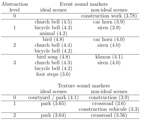
Abstraction Event sound markers
level ideal scenes non-ideal scenes
0 construction work (3.78)
church bell (4.5) car horn (3.9)
1 bicycle bell (4.3) siren (3.9)
animal (4.2)
bird (4.8) car horn (4.0)
2 church bell (4.4) siren (4.0)
bicycle bell (4.2)
bird song (4.8) klaxon (4.1)
3 church bell (4.3) siren (4.0)
bicycle bell (4.2) foot steps (3.6)
Texture sound markers
ideal scenes non-ideal scenes
0 courtyard / park (4.1) construction (3.9)
1 park (3.65) crossroad (3.6)
construction vehicule (3.3)
2 park (3.64) crossroad (3.56)
Table 3: Event and texture classes identified as sound markers. In each cell, markers are ranked as decreasing order of V-test value, shown between parenthesis. p ≤ 0.01 for all sound markers.
same task using actual sound samples that they can listen to. The fact that subjects in our experiment are faced to the acoustic reality of the sounds for composing the environment may have decreased the socio-cultural impact. Other studies that considered sounds as stimuli have shown that the bus class can have a negative influence on the assessment of the environment, see Lavandier & Defr´eville (2006).
Sound markers
We have shown that, from a qualitative point of view, the composition of the scenes in terms of sound sources differs between ideal or non-ideal scenes. We now investigate whether some of the sound classes are specific to a given en-vironment. For that purpose, the V-test detailed in Section 3.4 is considered separately for each abstraction level. Results are presented in Table 3.
lev-els. As shown on Figure 5, classes related to human presence (male footsteps on concrete, bicycle bell ), and of nature (animals, bird, and bird song) are ideal scenes markers as well as the church bell class. This latter result may be due to the socio-cultural background of the subjects who are mostly Eu-ropean citizens. In fact, according to Schafer, a sound that is identified by a person as being an important element of his/her environment, is well ac-cepted. Sound markers of non-ideal scenes are classes related to construction sites (construction works), or suggesting intense traffic (horn, siren).
Regarding textures, 5 markers are identified. For the ideal scenes, those are classes related to subdued or quiet ambiances (courtyard, park ). The marker classes for the non-ideal scenes are, as for the events, related to construction sites (construction, construction vehicle), together with a class related to traffic (crossroads).
Although the whole set of identified markers are rather intuitive, none of the event classes related to the noise of motor vehicles are identified as markers, except for the texture class crossroads. To generate an unpleas-ant traffic, subjects chose the classes horn or siren. We thus conclude that isolated motor vehicle sounds are understood as being part of the urban en-vironment, and thus their nature is not necessarily linked to an unpleasant soundscape.
Representation space induced by semantic features
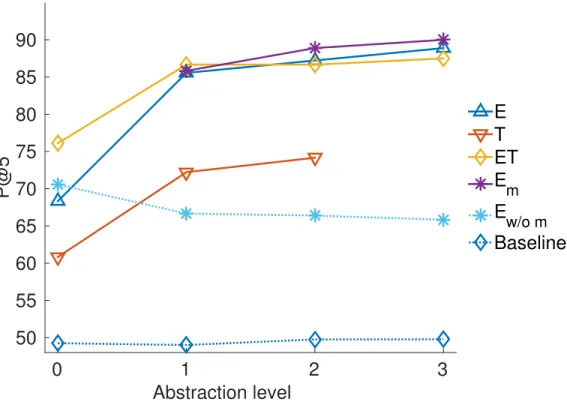
In this section, we evaluate at which level a semantic representation of the scenes allows us to discriminate between the two types of environments. For this purpose, a rank 5-precision is computed on the space induced by the semantic features S, and for each abstraction level (see Section 3.4). The vectors S are built by using all the classes (ET ), only the event classes (E), only the texture classes (T ), only the event classes corresponding to sound markers (Em), or only the event classes excluding sound markers (Ew/o,m).
Texture classes corresponding to sound markers are not numerous enough to reliably compute the metric, and are thus not considered. For the same reasons, event classes corresponding to sound markers at abstraction level 0 are also discarded. Results are shown on Figure 6.
Concerning ET , the rank 5-precision is 76% at abstraction level 0 (the most abstract), and remains above 86% for subsequent abstraction levels. Considering only the presence / absence of sound classes thus allows us to properly discriminate between the two types of environments. We also notice
Abstraction level 0 1 2 3 P@5 50 55 60 65 70 75 80 85 90 E T ET E m E w/o m Baseline
Figure 6: Rank 5-precision (P @5) obtained by considering the dissimilarity matrix com-puted from the paired Hamming distances of the semantic features vectors as a function of the abstraction level. The vectors are built by using all the classes (ET ), only the event classes (E), only the texture classes (T ), only the event classes corresponding to sound
markers (Em), or only the event classes excluding sound markers Ew/o,m. Baseline results
are achieved by considering random vectors as input.
that the less abstract (and therefore more precise) the description is, the more effective it is to predict agreement.
Considering E and T separately, it appears that: 1) the rank 5-precision obtained with E is similar to the one obtained with ET ; 2) the rank 5-precision obtained with T is always lower than the one obtained with E, by 10% to 15%. Those results indicate that the semantic information that is discriminative is mostly carried by the events. Those results are in line with results of Maffiolo (1999). As discussed in Section 2.1, it seems that humans analyze the event scenes which are composed of several sound events in a descriptive manner, i. e. by identifying the sources.
The dimension of the vectors S for Em is lower than the dimension of
the classes are considered (ET ). S being a boolean vector, the smaller the dimension, the lower the amount of information it can carry. Despite this, it appears that the rank 5-precision obtained with Em is equal – or superior –
to the ones obtained with E or ET , although only a partial information is used in that case to describe the scenes. Reciprocally, if the sound markers are not taken into account for the description (Ew/o,m), the performance is
below the one achieved when considering only the textures as features. Thus, most if not all of the semantic information allowing to differentiate between ideal and non-ideal scenes is included in the markers.
To sum up, the outcomes of this analysis are:
1. unlike what we outlined with the sound levels, a semantic description of the scenes composition in terms of presence / absence of sound sources allows us to reliably differentiate between the two types of environments (ideal or non-ideal);
2. the semantic information is mainly contained in the event sound classes; 3. only a part of the event classes, i. e. the sound markers, are useful to
differentiate between the ideal and non-ideal scenes.
Since we have extracted the typical classes of the ideal and non-ideal scenes and verified that the distinction between those two types of scenes was largely dependent on the presence of these classes, we shall now investigate whether a description of the scenes only based on the sound pressure level of these sound markers could characterize the perceived pleasantness, perhaps better than a globally computed sound level.
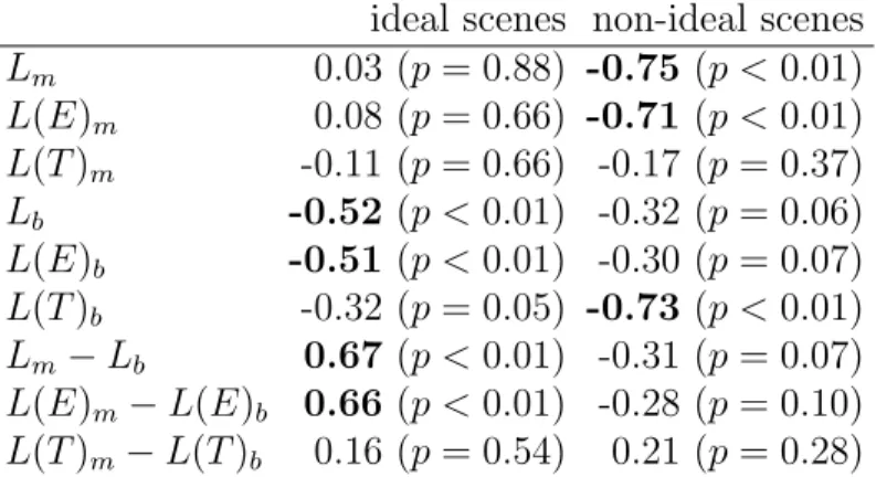
Influence of sound marker levels on the perceived pleasantness To do so, the correlations between Ascene and the sound levels are evaluated.
In this section, the sound levels are computed by taking into account only the previously identified sound markers. We define Lm (resp. L(E)m and
L(T )m), the sound level computed by taking into account only the sound
markers, and Lb (resp. L(E)b and L(T )b), the sound level computed by
taking into account all the sound classes, except the sound markers. When the feature characterizes an ideal scene (resp. non-ideal scene), only the markers identified for the ideal scenes (resp. non-ideal scenes) are considered. We henceforth call ideal markers and non-ideal markers the two types of markers. Results are shown on Table 4.
ideal scenes non-ideal scenes Lm 0.03 (p = 0.88) -0.75 (p < 0.01) L(E)m 0.08 (p = 0.66) -0.71 (p < 0.01) L(T )m -0.11 (p = 0.66) -0.17 (p = 0.37) Lb -0.52 (p < 0.01) -0.32 (p = 0.06) L(E)b -0.51 (p < 0.01) -0.30 (p = 0.07) L(T )b -0.32 (p = 0.05) -0.73 (p < 0.01) Lm− Lb 0.67 (p < 0.01) -0.31 (p = 0.07) L(E)m− L(E)b 0.66 (p < 0.01) -0.28 (p = 0.10) L(T )m− L(T )b 0.16 (p = 0.54) 0.21 (p = 0.28)
Table 4: Linear correlation coefficients computed between mean perceived pleasantness Ascene (Exp. 1.b) and sound levels related to the presence of sound markers.
Concerning the sound levels, the same trends are measured between Lm, L(E)m and L(T )m on one side, and L, L(E) and L(T ) on the other side,
see Figures 7a and 7d. No matter whether all the classes or only the markers are considered, it appears that:
1. a significant difference between levels of ideal and non-ideal scenes ex-ists (Lm, L(E)m and L(T )m: p < 0.01);
2. the sound level of scenes is mainly related to the sound events, com-pared to the textures;
3. the sound level of events has an influence on the perception of pleas-antness for non-ideal scenes, but not for ideal scenes;
4. the sound level of textures does not play any role in the perception of the pleasantness.
To conclude, the level of non-ideal markers has a negative influence on the pleasantness for the non-ideal scenes. On the other hand, the level of ideal markers does not influence the perceived pleasantness for the ideal scenes.
Considering the non markers classes, we can observe on the ideal scenes results, a weak negative correlation for Lb (r = −52, p < 0.01) and L(E)b
(r = −51, p < 0.01), see Figures 7b and 7e. It is the first time that an objective feature allows us to define the pleasantness of ideal scenes. This leads us to conclude that the level of non-typical sound classes of a pleasant environment has a negative influence on the pleasantness.
(a) ni i Lm -60 -55 -50 -45 -40 -35 -30 -25 -20 (b) ni i Lb -60 -55 -50 -45 -40 -35 -30 -25 -20 (c) ni i Lm ! Lb -30 -25 -20 -15 -10 -5 0 5 10 15 (d) Ascene -3 -2 -1 0 1 2 3 Lm -60 -55 -50 -45 -40 -35 -30 -25 -20 (e) Ascene -3 -2 -1 0 1 2 3 Lb -60 -55 -50 -45 -40 -35 -30 -25 -20 (f) Ascene -3 -2 -1 0 1 2 3 Lm ! Lb -30 -25 -20 -15 -10 -5 0 5 10 15
Figure 7: Distribution of the relative sound levels related to the presence of markers Lm
(a, d), Lb (b, e) and Lm− Lb(c, f), versus scene type (i: ideal, ni: non-ideal) (a, b, c) and
perceived pleasantness Asceneof experiment 1.b (d, e, f).
Moreover, whereas L(T ) did not show any significant correlation for non-ideal scenes, a strong negative correlation is observed for L(T )b (r = −0.73,
p < 0.01). This indicates that the level of non-marker texture classes does not influence the perceived pleasantness in the same way for ideal and non-ideal scenes. Sound level of textures seems to have a negative effect for the non-ideal scenes, and no significant effect for the ideal scenes.
A last group of features is now considered, namely Lm − Lb, L(E)m−
L(E)b and L(T )m− L(T )b. These features describe the difference between
the markers level and those of the other sound classes, see Figures 7c and 7f. They express the saliency of the markers with respect to the sound mixture. For the ideal scenes, a moderate positive correlation is observed for Lm− Lb (r = 0.67, p < 0.01) and L(E)m − L(E)b (r = 0.66, p < 0.01). For
the non-ideal scenes no correlation is observed. Thus, for the ideal scenes, it is not the absolute markers level that is important, but their relative level with respect to the other sounds composing the scene. A double perceptual mechanism for the ideal environments can thus be observed:
• the higher the absolute level of sounds not being ideal markers, the weaker the pleasantness,
• the higher the relative level of ideal markers compared to the remaining sounds, the higher the pleasantness.
On the contrary, the fact that we observe for the non-ideal scenes both significant correlations for Lm and L(E)m and no correlation for Lm− Lb and
L(E)m - L(E)b, shows that it is indeed the absolute level that matters for
non-ideal environments.
3.6. Discussion
From this analysis, the following points can be outlined:
• differentiating ideal and non-ideal scenes: the semantic features, and the global sound levels (L, L(E) and L(T )), allow us to differentiate reliably between ideal and non-ideal scenes. The semantic description seems to be more powerful;
• events or textures: whatever the feature type, be it semantic or related to the sound pressure level, events are the most useful components of the scene to differentiate the two types of scenes; textures bring a limited amount of information;
• pleasantness prediction: considering the correlation between sound lev-els and pleasantness, it seems that the way subjects perceived the qual-ity of a given environment depends on its very nature (ideal or non-ideal). From the data gathered in those experiments, the same set of features cannot be considered to predict the pleasantness of ideal and non-ideal scenes:
– for non-ideal scenes, the global levels (L and L(E)), or the level of sound markers (Lm and L(E)m), have a negative influence on
pleasantness. Taking into account the contribution of each of the different sources of the scene does not improve the prediction per-formance compared to a global analysis of the environment. – for ideal scenes, on the contrary, the sound markers characteristics
and those of the other sounds have to be considered separately to predict the pleasantness. The markers level relative to the back-ground noise (L(E)m−L(E)b and Lm−Lb) is positively correlated
to the pleasantness, whereas the noise level (Lb and L(E)b) is
neg-atively correlated.
The fact that the pleasantness of the ideal scenes is not correlated to global physical features, contrary to the pleasantness of non-ideal scenes, has also been studied recently by Gozalo et al. (2015).
We can assume two perceptual modes of operation that involve different types of features and rely on the hedonic nature of the stimuli. It thus appears that the features considered for the pleasantness judgment also depends on a preliminary judgment of the global hedonic nature of the environment (ideal or non-ideal).
A similar phenomenon is observed for the perception of textures, see Section 2.1. It seems that the brain selectively adapts the way it encodes the information (statistic summary for textures, finer description for events) following a previous decision making process based on the nature of the stimuli, i. e. is it an event or a texture ?
Another hypothesis would be that the volume somehow acts as an he-donic ”gain” factor. If the volume of a negative marker is high, it lowers the overall pleasantness. If the volume of a positive marker is high, it increases the overall pleasantness. Evidently, the positive gain is expected to saturate at a given level and will quickly decreases as the level raises above a given threshold.
4. Experiment 2: modification of the semantic
content
4.1. Objective
The previous experiment demonstrated that, among the classes of sounds oc-curring in urban soundscapes, those gathering markers are specific to some
environments. Those sound markers seem to have a great impact on percep-tion. This impact is studied here in more detail using an added benefit of the simulation paradigm proposed in this paper, the ability to manipulate and modify the generated scenes.
In order to investigate deeper into the relation between the pleasantness of ideal and non-ideal scenes and the sound markers, the audio waveforms of the simulated scenes are regenerated without the classes identified as markers. To do so, ideal markers are removed from the ideal scenes, and non-ideal markers are removed from the non-ideal scenes. To evaluate the impact on the perception of pleasantness caused by those modifications, a perceptual test is conducted with a protocol close to the one considered in experiment 1.b.
The objective of this experiment is to study if the removal of the previ-ously identified markers has an impact on the perceived pleasantness. Two hypothesis are thus formulated:
• for the non-ideal scenes, we hypothesize that the absence of non-ideal markers will increase the pleasantness score;
• for the ideal scenes, we hypothesize that the absence of the ideal mark-ers will decrease the pleasantness score.
If the first hypothesis is rather intuitive, the second is less. Indeed, it is not obvious that the removal of the ideal markers, though perceptively positively connoted, will decrease the global quality of a soundscape, since this removal also decreases the global sound level of the scene. However, as discussed before, the global amplitude level can only be considered as a partial indicator of pleasantness of the ideal soundscapes. Furthermore, the level of ideal markers positively impact the pleasantness. For those reasons, the validation of the second hypothesis is of high interest.
4.2. Planning of experiment 2
StimuliThere are 144 stimuli of 30 seconds duration. More precisely:
• 72 scenes with markers: the 72 scenes originally simulated by the sub-jects of experiment 1.a where the sound classes identified as markers are kept.
• 72 scenes without markers: 72 scenes where the sound classes identified as markers are removed.
Notwithstanding the presence or absence of markers, the scenes with and without markers are exactly the same.
In order to create the marker-less scenes with still some sound diversity and no absence of sound activity for long periods within the scene, only the sound classes of events of the first level of abstraction are removed, see Table 3. Those classes are:
• church bell, bicycle bell, and animals for the ideal scenes without mark-ers;
• siren, car horn for the non-ideal scenes without markers.
Thus, only part of the ideal and non-ideal markers are removed from the scenes without markers.
Procedure
The subjects evaluate the 144 scenes. The evaluation is done on a 11-point bipolar semantic scale ranging from -5 (non-ideal / very unpleasant) to +5 (ideal / very pleasant). Before rating a scene, subjects must listen to the first 20 seconds. After scoring, they are free to move on to the next scene.
For each subject, the scenes are presented in a random order. The first 10 scenes allow the subject to calibrate their scores. Those calibration scenes are 5 ideal scenes with markers and 5 non-ideal scenes with markers. These first 10 scenes are replayed at the end of the experiment, and only the scores given at the second occurrence are taken into account.
The experiment is scheduled to last 1 hour. The subjects do not know the nature of the scenes.
Apparatus
All the subjects performed the experiment on standard desktop computers with the same hardware and software configurations. The audio files were played in diotic conditions by semi-open headphones Beyerdynamic DT 990 Pro. The output sound level was the same for all the subjects.
All the subjects performed the experiment simultaneously in a quiet environment. They were not allowed to talk to each other during the exper-iment.
An experimenter was available during the whole duration of the exper-iment in order to assist subjects and to answer questions.
Subjects
12 subjects performed the experiment (8 male, 4 female; averaging 29.5 years of age, s.d. of 14 years). All the subjects had been living in Nantes, France, for at least two years at the time of the experiment and reported normal hearing. None of them took part in the previous experiments 1.a and 1.b.
All the subjects succeeded in doing the experiment.
4.3. Data and statistical analysis
The type of data analyzed in this experiment have been considered for ex-periment 1.a, see Section 3.4 for details.
The aim here is to validate the hypothesis that the removal of ideal and non-ideal markers has a significant effect on the perceived pleasantness. To do so, we perform an analysis of variance (ANOVA). We consider Asubject
as a dependent variable, and the type of environment (ideal or non-ideal) as well as the presence/absence of markers as independent variables. As each subject evaluated the whole set of scenes, a two factors repeated measures ANOVA with interaction is used to evaluate whether there exist a significant difference of perceived pleasantness between the scenes with and without markers. The two independent variables are considered as within-subject factors. The factors being of only two levels each (type: ideal or non-ideal, marker: with or without), the sphericity hypothesis does not need to be checked. Post hoc analyses are done using the Tukey-Kramer procedure.
All statistical significance tests are conducted with a critical threshold of α = 0.05
4.4. Results
4.4.1. Outliers detection
Let us consider Asubject for the scenes with markers, see Figure 8a. Close
(a)
i/km ni/km i/rm ni/rm -5 -4 -3 -2 -1 0 1 2 3 4 5 (b)
i/km ni/km i/rm ni/rm -5 -4 -3 -2 -1 0 1 2 3 4 5
Figure 8: Distribution of the mean perceived pleasantness per subject Asubject (a) and
the mean perceived pleasantness per scene Ascene (b) versus scene type (i: ideal, ni:
non-ideal, km: with markers, rm: without markers). Black stars in subfigure (a) stand for the detected outlier, i. e. subject 7.
from the others’. This subject evaluated positively more than half of the non-ideal scenes with markers (see Annex Appendix B, subject 7). He gave a score above 0 for 58% of the non-ideal scenes with markers, contrary to an average of 11% for the other subjects.
Furthermore, this subject used the whole scale (from -5 to 5) to score both the ideal scenes and the non-ideal scenes. Those behaviors strongly differ with the ones of the other subjects, be they from this experiment or the previous ones. Subject 7 is thus discarded from the analysis.
4.4.2. Influence of the markers on perceived pleasantness
In this section, we study the scores given by the subjects while listening to the different types of scenes, namely the ideal scenes with markers, non-ideal scenes with markers, non-ideal scenes without markers and non-non-ideal scenes without markers, see Figure 8b. The repeated measures ANOVA applied to
Asubject shows a significant effect of the environment type (F [1, 10] = 175,
p < 0.01), of the presence/absence of markers (F [1, 10] = 7, p < 0.05), and of the interaction between those two factors (F [1, 10] = 67, p < 0.01).
The post hoc analysis exhibits significant differences between all groups of observations, notably between the ideal scenes with markers and the ideal scenes without markers (p < 0.05) as well as between the non-ideal scenes with markers and the non-ideal scenes without markers (p < 0.01).
Those results indicate that the removal of the markers indeed modify the perception of the scenes by the subjects, see Figure 8. Our two hypotheses are thus verified :
• the removal of ideal markers improved the pleasantness of the non-ideal scenes;
• the removal of ideal markers reduced the pleasantness of the ideal scenes.
The significant interaction shows that the type of environment influ-ences the effect of the presence/absence of the markers. Indeed, the average difference of Asubject between the scenes with markers and the scenes without
markers is larger for the non-ideal scenes (1.1) than for the ideal scenes (0.5).
4.5. Discussion
This experiment shows that the presence of the markers identified during the analysis of experiment 1 does have an impact on the perceived pleasantness. The removal of the non-ideal markers has a positive effect on the perception of the non-ideal scenes. Perhaps more surprisingly the removal of the ideal markers slightly decreases the perception of the ideal scenes: this is a more striking observation since, due to the removal of the markers, the acoustic pressure level of the ideal scenes with markers is higher than the one of the ideal scenes without markers.
This strongly confirms that ideal markers do have a positive impact on the perception of an environment. The fact that their removal decreases
Asceneindicates that it should be possible to improve the perceived
pleasant-ness of a given urban area by the addition of sounds commonly considered as pleasant such as bird calls. Those conclusions are in line with the positive approach introduced by Schafer (1977).
5. Outcomes for soundscape perception
This series of three experiments showed that most of the descriptors used in this study, be they of a semantic or acoustic nature, allow us to distinguish between an ideal scene and a non-ideal one.
That being said, we observe that the physical characteristics correlated with the perceived pleasantness clearly differ depending on the type of scenes. In the case of ideal scenes, it is above all the emergence of sound markers that determines the perceived quality, whereas in the case of non-ideal scenes, it is the overall sound level that prominently influences it.
These results show that the perception of the qualities of a scene indeed depends primarily on its identifiable sound sources. The characteristics that are taken into account during the perceptual process appear to vary from one source to the other, from one type of environment to the other. This fact leads the authors to believe that there is little hope to find a holistic physical descriptor that can adequately account for the affective qualities of all types of sound environment.
Those results may have an impact on the relevant strategies to adopt while trying to improve the quality of a sound environment:
• in the case of non-ideal scenes, one should focus on reducing the acous-tic pressure level, whether globally, or by discarding specific sources such as sirens or car horns
• in the case of ideal scenes, one should first identify which sources are pleasant to the targeted community, second lower the volume of the other sound sources, and, if possible, raise the contribution or add positive sound markers.
Finally, this work allows us to conjecture as to the nature of the mental representations of the concepts ”pleasant urban sound environment” and ”unpleasant urban sound environment” .
First, the fact that the semantic information (which sound source is present) and structural information (at which level) are different for ideal and non-ideal scenes leads us to believe that these two types of information characterize the above cited concepts.
Second, the fact that the removal of sound markers changes the per-ceived pleasantness leads us to believe that the abstract concept related to pleasantness depends on the activation of a network of concepts strongly