1
Modeling Tropical Cyclone Boundary Layer:
Height-1
Resolving Pressure and Wind Fields
2
Reda Snaiki, Teng Wu
*3
Department of Civil, Structural and Environmental Engineering, University at Buffalo, State
4
University of New York, Buffalo, NY 14126, USA
5
*Corresponding author. Email: [email protected]
6
Abstract: The high-accurate wind field of a tropical cyclone boundary layer, which is essentially
7
governed by the Navier-Stokes equations, could be efficiently obtained by predefining the pressure
8
field. Conventionally, the prescribed pressure filed is a 1-D function varying with the distance to
9
the cyclone center (radius). In this study, the pressure field model has been extended to a 2-D
10
function with respect to both radius and height. In addition, a number of field measurements in the
11
tropical cyclone boundary layer indicate rapid variation of the thermodynamic temperature and
12
moisture with time and space. Hence, their effects on the wind field were considered in terms of
13
the virtual temperature, which was integrated in the modeling of pressure field. The analytical
14
solutions of the wind field, as a sum of gradient and frictional wind components, were derived
15
based on a height-resolving scheme using the updated pressure field. Since the tropical cyclone
16
gradient wind and depth of boundary layer are mutually dependent, the iteration approach was
17
utilized in the computation. The proposed height-resolving pressure and wind analytical models
18
have been comprehensively validated with the global positioning system (GPS)-based dropsonde
19
data. The significant importance to consider the height-varying pressure, thermodynamic
20
temperature and moisture in the modeling of the wind field in the tropical cyclone boundary layer
21
were also demonstrated.
22
Keywords: Tropical cyclone, Height-resolving model, Boundary layer wind, Pressure,
23
Temperature, Moisture.
2
1. Introduction
25
The wind field in the boundary layer region of a mature tropical cyclone is of great significance
26
since a substantial part of economic and life losses result from the events directly or indirectly
27
related to high winds, e.g., wind damage to structures, wind-driven storm surge and wind-rainfall
28
interaction. The situation has become more challenging due to the changing climate and continued
29
escalation of coastal population. While there have been considerable advances in improving the
30
simulation accuracy of tropical cyclone wind field based on the numerical weather prediction
31
models associated with a significant increase of observation data, they are not practical to be
32
employed in the assessments of risk posted by wind-related hazards due to their high
33
computational demands. The state-of-the-art wind hazard risk analysis is essentially based on the
34
Monte Carlo methodology proposed by Russel (1971), where a large number of scenarios need to
35
be carried out. In this context, the parametric, engineering models for tropical cyclone wind fields,
36
based on the prescribed pressure fields, have been popularly utilized.
37
While several studies have shown that the height-resolving models are superior to the slab
38
(depth-averaged) models that treat the boundary-layer height of the tropical cyclone as a constant,
39
both of these two high-efficient wind field simulation schemes are widely employed in engineering
40
applications. Although the hydrostatic equation simply indicates the pressure field depends on the
41
height, both the slab and height-resolving models conventionally assume the prescribed pressure
42
field is unchanged through the depth of the boundary layer. In particular, the 1-D empirical model
43
introduced by Holland (1980) for pressure, varying with the distance to the cyclone center (radius),
44
has been extensively used due to its simplicity and consistency with field measurements (e.g., Zhao
45
et al. 2013; Mudd et al. 2014). Recently, Huang et al. (2012) integrated the effects of temperature
46
and variation of central pressure difference with height into the prescribed pressure field for more
3
accurately simulating the typhoon wind field using Meng’s model (Meng et al. 1995). Since the
48
gradient wind speed in this refined Meng’s model varies with the height from the ground, it is not
49
easy to select the appropriate value in the calculation.
50
Following the pioneering work of Huang et al. (2012), the 1-D Holland’s empirical
51
pressure model has been extended to a 2-D function with respect to both radius and height in this
52
study. Since a number of field measurements in the tropical cyclone boundary layer indicate rapid
53
variation of the thermodynamic temperature and moisture with time and space, their effects on the
54
wind field were considered in terms of the virtual temperature, which was integrated in the
55
modeling of pressure field. The obtained 2-D formula for pressure p z r
, explicitly includes the56
temperature lapse rate parameter . The global positioning system (GPS)-based dropsonde data
57
(e.g., temperature, humidity, pressure) for the tropical cyclones further demonstrated a heavy
58
dependence of and hence pressure on the moisture content. Furthermore, the proposed 2-D
59
pressure formula indicates the consideration of climate changes (e.g., global warming) may have
60
significant implications to the wind field simulation of a tropical cyclone. The analytical solutions
61
of the wind field were derived based on a recently developed height-resolving scheme (Snaiki and
62
Wu 2016) using the obtained 2-D pressure field. To select an appropriate height for the calculation
63
of gradient wind speed, the iteration approach was utilized using the depth scale of the tropical
64
cyclone boundary layer as the initial value. The proposed height-resolving pressure and wind
65
analytical models have been comprehensively validated with the GPS-based dropsonde data. The
66
significant importance to consider the height-varying pressure, thermodynamic temperature and
67
moisture in the modeling of the wind field in the tropical cyclone boundary layer were also
68
demonstrated.
69 70
4
2. Height-resolving pressure field
71
In the simulation of the wind field inside the boundary layer of a tropical cyclone, the surface level
72
pressure profile is typically prescribed to efficiently solve the horizontal momentum equations. In
73
general, the atmospheric pressure can be expressed by the state equation for ideal gas as follows:
74
pRT (1)
75
where
= air density; R = ideal gas constant; and T = temperature.76
2.1 Moisture effects
77
The warm, moist air is considered as the fuel of the tropical cyclones. To simultaneously account
78
for the temperature and moisture effects, a convenient way to proceed would be the use of the
79
virtual temperature T which is expressed as follows: v
80
1
noa v v v noa v R r R T T R r (2) 81where r = mixing ratio of water vapor; v R = gas constant of the water vapor; and v
82
1 1
287
noa J kg K
R is the gas constant of mixture of nitrogen (N
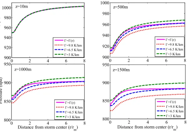
2), oxygen (O2) and argon (Ar).
83
noa
R will be denoted subsequently by R for convenience. Accordingly, the state equation can be
84
extended to include the virtual temperature:
85
v
pRT (3)
86
The importance of moisture consideration in the pressure simulation for a typical tropical
87
cyclone will be illustrated through two dropsonde measurements collected by the National
88
Hurricane Center and Hurricane Research Division during hurricane Katrina. The dropsonde IDs
89
are (051926111) and (051926170), respectively. The dropsondes are usually launched from an
5
altitude of 3 km or higher and provide high-resolution thermodynamics data, namely temperature,
91
pressure, and humidity. To ensure quality control, collected data are post-processed. Figure 1
92
presents the pressure p as a function of humid air*Tv and of dry air*T, respectively. It is shown the
93
consideration of moisture gives a slope of 285.6 that is close to the gas constant R287 J kg K1 1
94
, while the dry assumption results in a slope much larger than this value. This indicates the
95
importance of moisture to accurately simulate the pressure field in the tropical cyclone.
96
97
Fig. 1 Moisture effects on the state equation based on two dropsonde measurements during hurricane Katrina (Left:
98
051926170 and Right: 051926111)
99
2.2 Pressure formula
100
To derive the pressure expression, the state equation is first applied on the surface level which
101 gives: 102 0 0 v0 p RT (4) 103
where 0= surface air density; and T =surface virtual temperature. v0
104
Combining the Eqs. (3) and (4) yields the following expression:
105 260 280 300 320 340 360 380 400 820 840 860 880 900 920 940 *Temperature(K.kg/m3) P re ss ur e (h pa ) 260 280 300 320 340 360 380 400 840 860 880 900 920 940 960 *Temperature(K.kg/m3) P re ss ur e (h pa )
With moisture: Slope =285.6 Without moisture: Slope=1825
With moisture: Slope =286.8 Without moisture: Slope=1791
6 0 0 0 v v T p p T (5) 106
The surface pressure is given based on the widely-used Holland’s formula:
107
0 0 0. / B c m p p p exp r r (6) 108where p = central pressure at the surface; c0 = central pressure difference at the surface; p0 r = m
109
radius of maximum winds; r = radial distance from the tropical cyclone center; and B = Holland’s
110
radial pressure parameter. Hence the pressure can be expressed as:
111
0 0
0 0 . / B v c m v T p p p exp r r T (7) 112On the other hand, it is well known that temperature of air decreases with height. More
113
specifically, it is approximately a linear function of height for relatively low altitudes, as shown in
114
Fig. 2. The data in Fig. 2 is provided by the dropsonde (01074007) during hurricane Katrina.
115
116
Fig. 2. Temperature profile of hurricane Katrina corresponding to the dropsonde ID (01074007)
117
Accordingly, the temperature could be approximated as:
118
0
v v
T z T (8)
119
where z= vertical coordinate; and = temperature lapse rate. Therefore, the pressure formula
120 290 295 300 305 310 0 200 400 600 800 1000 1200 Tv (K) H ei gh t ( m )
7 becomes: 121
0 0
0 0 1 c . m / B v p z p p exp r r T (9) 122If the moisture was disregarded, one could determine the value of the so-called dry
123
adiabatic lapse rate for dry simulation according to the first law of thermodynamics
124
1
p
dq c dT dp
, where cp= specific heat capacity of air; dq = heat transfer =0; and dp gdz
125
based on the hydrostatic equation. As a result, the dry adiabatic lapse rate can be obtained as
126 follows: 127 9.8 d p dT g K Km dz c (10) 128
For a typical tropical cyclone, however, it is noted that the temperature lapse rate changes with
129
space. Hence, constant cannot be adopted for the pressure simulation. Figure 3 presents the d
130
radial variation of the lapse rate for hurricane Gustav (2008) based on 62 dropsondes data.
131
132
Fig. 3. Radial variation of the observed lapse rate for hurricane Gustav (2008)
133 0 100 200 300 400 500 600 700 800 3 3.5 4 4.5 5 5.5 6 6.5 7 Radius (km) L ap se r at e (K /k m ) Observed Rankine-like profile of Holland-like profile of
8
As shown in Fig. 3, the lapse rate varies considerably with the distance from the center of the
134
tropical cyclone. The variation is reasonable since the moisture causes the lapse rate to be smaller
135
(CCSP 2006; IPCC 2000; 2007; 2012). Actually, the lapse rate parameter is an important
136
parameter in the meteorology science to consider the negative feedback from global warming and
137
hence increased moisture (IPCC 2000; 2007; 2012). In the eyewall region where the moisture
138
content is high, there is a rapid drop in the lapse rate (around 3 /K km ). Then the moisture content
139
tends to decrease far away from the eye wall, which leads to an increase of the lapse rate reaching
140
a value around 6.5 /K km . Similarly, a reduced moisture content results in increase of the lapse
141
rate in the eye region compared to the eye wall region. There is a sudden decrease of the lapse rate
142
in some regions far away from the tropical cyclone center, as presented in Fig. 3 (around
143
400
r km). This is probably because these specific dropsondes were launched in a rainband
144
region where the moisture content was locally increased. It should be noted that only the radial
145
variation of the lapse rate is illustrated in Fig. 3, while, in general, it is also dependent on the
146
azimuthal coordinate. The temperature lapse rate in the tropical cyclone is typically smaller than
147
the dry adiabatic lapse rate d 9.8K Km.
148
Based on the measured data shown in Fig. 3, two empirical radial profiles of are
149
proposed in this study for convenient applications to the pressure simulations in the tropical
150
cyclone. The first formula is a modified version of Rankine-like profile, which leads to the
151
following expression for the lapse rate:
152 0 0 ( ) ; ( ) ( ) ; m m r eye eye m m a m r m r r r r r r r r r (11) 153
9
where
m
r
= lapse rate at the radius of maximum winds; = lapse rate at the tropical cyclone eye
154
center; = lapse rate in the far field; a = scaling parameter that adjusts the profile shape. The 0
155
second formula can be obtained using a modified version of Holland-like profile, which leads to
156
the following expression:
157
0.5 0 0 ( ) exp 1 b b m m rm r r r r r (12) 158where b= scaling parameter that adjusts the profile shape; is assumed to be approximately eye
159
equal to for simplification. In general, Eq. (12) provides a smoother profile than that generated 0
160
by Eq. (11). The measured data of hurricane Gustav (2008) were fitted using the abovementioned
161
empirical profiles [i.e., Eq. (11) and Eq. (12)] with parameters of 2.8 /
m
r K km
,
162
0 eye 6.8 /K km
and a0.77 for the Rankine-like profile and 3.3 /
m
r K km
, 0 6.55 /K km 163
and b1.11 for the Holland-like profile. The fitted profiles are shown in Fig. 3, and the one based 164
on the Holland-like formula presents a better result according to least squares. It should be stressed
165
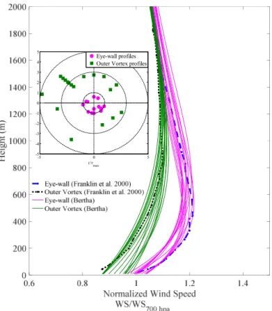
out that the proposed empirical profiles of the lapse rate can be further improved with more data
166
from the dropsondes.
167
Figures 4 and 5 present, respectively, the radial and vertical pressure profiles based on the
168
proposed 2-D model [Eq. (9)] with various considerations of the lapse rates. The radial variation
169
of the temperature lapse rates is obtained using the Holland-like profile. The other parameters are
170
as follows: pc0 950hpa; rm 55km; B ; and 1 Tv0 302K. It is shown that the effects of the
171
changing temperature lapse rate cannot be ignored to accurately simulate the pressure profiles in
172
the tropical cyclones.
10 174
Fig. 4. Radial pressure profiles for several lapse rates at different altitudes
175
As shown in Fig. 4, the correlation of the radial pressure profile with the lapse rate increases with
176
the height. In the eyewall region, the proposed pressure profile
( )r
is almost identical to177
the pressure profile corresponding to 3K km/ , while it coincides with the pressure profile
178
corresponding to 6.5 /K km far away from the tropical cyclone center. This observation is
179
further demonstrated by the vertical pressure profiles as presented in Fig. 5. In addition, Fig. 5 also
180
clearly shows that larger differences of the pressure values are obtained at higher altitudes.
181 0 2 4 6 8 900 920 940 960 980 1000 P re ss ur e (h pa ) z=10m =(r) =9.8 K/km =6.5 K/km =3 K/km 0 2 4 6 8 900 920 940 960 980 1000 z=500m =(r) =9.8 K/km =6.5 K/km =3 K/km 0 2 4 6 8 800 850 900 950
Distance from storm center (r/rm)
Pr es su re ( hp a) z=1000m =(r) =9.8 K/km =6.5 K/km =3 K/km 0 2 4 6 8 800 850 900 950
Distance from storm center (r/rm) z=1500m
=(r)
=9.8 K/km
=6.5 K/km
11 182
Fig. 5. Vertical Pressure profiles corresponding to several lapse rates at different locations inside the tropical
183
cyclone
184
Using the same data as in Fig. 1, the vertical pressure profile was simulated using the proposed
185
pressure profile [Eq. (9)]. It could be concluded that both the observed and simulated pressures are
186
in good agreement as illustrated in Fig. 6.
187 800 850 900 950 1000 0 500 1000 1500 H ei gh t ( m ) r=r m =(r) =9.8 K/km =6.5 K/km =3 K/km 8000 850 900 950 1000 500 1000 1500 r=2r m =(r) =9.8 K/km =6.5 K/km =3 K/km 800 850 900 950 1000 0 500 1000 1500 Pressure (hpa) H ei gh t ( m ) r=3r m =(r) =9.8 K/km =6.5 K/km =3 K/km 8000 850 900 950 1000 500 1000 1500 Pressure (hpa) r=4r m =(r) =9.8 K/km =6.5 K/km =3 K/km
12 188
Fig. 6. Comparison between the simulated and observed pressures corresponding to two dropsondes during
189
hurricane Katrina (Left: 051926170 and Right: 051926111)
190
It is interesting to notice that the developed pressure formula of Eq. (9) may offer an
191
improved method to assess the climate change impacts on the wind field of tropical cyclones. More
192
specifically, the climate change assessment could be considered in terms of the surface central
193
pressure and the vertical pressure profile. Based on the surface central pressure, the future
194
projections of the sea surface temperatures (SST) can be incorporated into the wind field
195
simulations using the relative intensity developed by Darling (1991). Recently, Mudd et al. (2014)
196
carried out simulations to quantify the climate change impact on the northeast US coastal region
197
with this methodology. As pointed out by Mudd et al. (2015), however, considering only the SST
198
will not give accurate results for climate change estimation. Several other environmental
199
parameters that can contribute significantly to the tropical cyclone intensity and are expected to
200
change with global warming, should be accounted for (e.g., air moisture content, temperature at
201 8000 850 900 950 200 400 600 800 1000 1200 Pressure (hpa) H ei gh t ( m ) Observed pressure Simulated pressure 850 900 950 1000 0 200 400 600 800 1000 1200 Pressure (hpa) Observed pressure Simulated pressure
13
higher altitudes). For example, the moisture content is believed to increase significantly with
202
global warming (IPCC 2000; 2007; 2012). This indicates reduced lapse rates (Frierson 2005),
203
which could be conveniently integrated into the wind field simulations with the proposed 2-D
204
pressure model.
205
3. Height-resolving wind field
206
A linear height-resolving wind field model recently developed by Snaiki and Wu (2016) will be
207
used in this study for wind field simulation. The model not only considers the radial variation of
208
the depth scale of the boundary layer but also accounts for the azimuthal dependence of wind field,
209
resulting an enhanced simulation of the real behavior of a moving tropical cyclone (Snaiki and Wu
210
2016). In this section, a brief discussion of the employed wind field model will first be presented
211
for completeness, followed with the improved wind field simulation by integrating the 2-D
212
pressure field.
213
The governing equation of the wind field could be described as follows:
214 1 . p f t v v v k v F (13) 215
where v = wind velocity; f = Coriolis parameter; k = unit vector in the vertical direction; and F =
216
frictional force. In order to solve Eq. (13), the decomposition method is used in which the wind
217
velocity (v) is expressed as:
218
g
v v v' (14)
219
where vg= gradient wind in the free atmosphere; and v'= frictional component near the ground
220
surface. Therefore two equations can be derived from Eq. (13):
14 1 . p f t g g g g v v v k v (15a) 222 . . . f t g g v v v v v v v k v F (15b) 223
Similar to Meng et al. (1995), the gradient wind pattern vg is assumed to move at the translation
224
velocity of the tropical cyclone c in the free atmosphere, thus the unsteady term can be expressed
225 as: . t g g v
c v . On the other hand, the unsteady term
t
v
in the tropical cyclone boundary layer
226
is usually considered significantly smaller than the turbulent viscosity and inertia terms, and hence
227
neglected.
228
3.1 Gradient wind speed
229
Equation (15a) could be solved straightforwardly in the cylindrical coordinate system (Georgiou
230
1985; Meng et al. 1995). Hence:
231
2 1/ 2 2 4 g csin fr csin fr r p v r (16) 232where = approach angle (counter clockwise positive from the East). The radial velocity is then
233
obtained from the continuity equation:
0 1r g rg v dr r v
which is usually disregarded as suggested234
by Meng et al. (1995) due to its insignificant effects.
235
3.2 Frictional wind speed
236
In the cylindrical coordinate, Eq. (15b) becomes:
237 2 2 2 1 2 g g v v u u u v v u w v K u u r r z r r (17a) 238
15 2 2 1 ' g g 2 ag v v v v v v u v v u u w u K v v r r z r r r (17b) 239
where ( , , )u v w = velocity vector; ', 'u v = frictional components of the wind velocity; 2 g g v f r is 240
the absolute angular velocity; g g
ag v v f r r
is the vertical component of absolute vorticity of
241
the gradient wind; and K = the turbulent diffusivity that is assumed to be a constant in this study.
242
The nonlinear Eqs. (17a) and (17b) could first be simplified using the scale analysis, and
243
then linearized as:
244 2 2 g g v u u v K r z (18a) 245 2 2 g g ag v v v v v u K r r z (18b) 246
The analytical solution for this linear system is presented as follows (Snaiki and Wu 2016):
247
1/2
( 0 ) (1 ) ( 1 )
0 1 1 0 1 1 ( , ) q z q z i q z i u z Real A e A e A e u u u (19a) 248
( 0 ) (1 ) ( 1 )
0 1 1 0 1 1 ( , ) q z q z i q z i v z Imag A e A e A e v v v (19b) 249 where 1 2 g K ; 1 2 ag K ; 1/ 2 1 (1 ) q i ; q1 (1 i) ; 1/ 2 1/ 4 0 q ; 250 1 2 g v K r ; 1 2 g v Kr ; and z’= new vertical coordinate used as the base of the computation scheme
251
where z’=0 is located above z10 (the 10 m height above the mean height of roughness elements)
252
(Meng et al. 1995). The other parameters are presented as follows:
253 3 0 1 2 4 X A X X X (20a) 254
16
*
1 * 0 0 1 1 4 i d icC e A A A K q q (20b) 255
*
1 * 0 0 1 1 4 i d icC e A A A K q q (20c) 256
2 2 2 2 1 0 2 * 2 * 1 1 1 1 2 4 4 d d d d C c C c C fr X q C K K K q q K q q (20d) 257
2 2 2 2 * 2 0 2 * 2 * 1 1 1 1 2 4 4 d d d d C c C c C fr X q C K K K q q K q q (20e) 258 2 3 2 2 d iC fr X K (20f) 259 * 4 0 0 2 2 d d d d C C fr fr X q C q C K K K K (20g) 260 2 1/2 4 csin fr r p r (20h) 261where Cd= drag coefficient; and (*) indicates a complex conjugate.
262
3.3 An improved wind field simulation for tropical cyclone
263
As mentioned in the preceding sections, the solution of the wind field could be conveniently
264
obtained by prescribing a pressure field that is unchanged with height (e.g., Meng et al. 1996;
265
Kepert 2001; Snaiki and Wu 2016). If the pressure variation with respect to the height is
266
considered, various gradient wind values corresponding to different heights need to be calculated.
267
This also leads to the mutual dependence of the gradient wind speed and the boundary layer depth.
268
To obtain the accurate value of the gradient wind in the wind field simulation of the tropical
269
cyclone, the iteration approach is utilized herein. In Snaiki and Wu (2016), the depth scale of the
270
tropical cyclone was highlighted to give good estimate of the height where turbulent fluxes tend
17
to become negligible. Specifically, three depth scales of the tropical cyclone, namely
14 0 1
272 , 1 2 1 1 and 1 2 1 1 corresponding to the frictional components
273
u v0, 0
,
u v1, 1
and
u v1, 1
[Eq. (19)], respectively, have been defined. Since,
u v0, 0
are the274
dominant frictional component, it is reasonable to select 0 as the initial value of the height of the
275
boundary layer. A systematic way to calculate the height-resolving wind field in this study is
276
illustrated in Fig. 7.
277
The first part of the flow chart of Fig. 7 is to determine the initial estimate of the boundary
278
layer height 0. Since 0 and the gradient wind speed depend on each other, the iteration process
279
is necessary. Once the initial guess for the boundary layer height 0 is determined, the
280
corresponding frictional wind speed components could be evaluated. The boundary layer height
281
will be updated until the contribution from the friction become negligible. Based on the obtained
282
boundary layer height i, the wind field at certain height will be calculated using two different
283
formulas. A constant value of the gradient wind speed evaluated at i is utilized for the locations
284
below the boundary layer height (i.e., z ). Otherwise (i.e., i z ), the gradient wind speed is i
285
a function of height z, and the frictional components are equal to zero.
18 287
Fig. 7. Flow chart of wind field simulation methodology
288
A simple wind field simulation example is presented in Fig. 8, where pc0 940 hpa;
289
40 m
r km; B1.2; c10 /m s; z0 0.0001; 50 2/
m
k m s; and
90 , to highlight the290
importance of considering the accurate gradient wind speed and boundary layer depth by iteration
291
method. The standard method indicates a constant value of the gradient wind speed is employed
292
in the wind field simulation.
19 294
Fig. 8. Simulation of the vertical wind profiles at different locations
295
As shown in Fig. 8, the vertical wind profiles simulated using the iteration and standard schemes
296
present large difference. The difference becomes more significant as the location is close to the
297
radius of maximum wind and tends to decrease far away from the center of the tropical cyclone. It
298
should be mentioned that the tangential wind speed vg in Huang et al. (2012) was considered to
299
vary with height from the ground surface rather than evaluated at the boundary layer depth, which
300
may need further improvement.
301
4. Model Validation
302
Wind records were obtained from the National Hurricane Center’s North Atlantic Hurricane
303
Database (HURDAT). Typically, the parameters needed for the simulation are: approach angle;
304
c translation velocity of the hurricane; p central pressure; pc central pressure difference; Rmax
305
radius of maximum winds; B Holland’s parameter;
latitude; and
longitude. The parameter306
max
R and B can be estimated using the methods available in the literature (e.g., Powell et al., 1991;
20
1998; Anthes 1982; Vickery et al., 2000b; Holland, 2008). In this study, the necessary information
308
is supplemented by the H*Wind snapshots. For the lapse rate parameters, the coefficients
m
r
,
309
eye
and can be approximated using the dropsonde data. 0
310
4.1 Surface wind simulation and validation
311
Two hurricanes, namely hurricane Bertha (1996) and Fran (1996) were selected for the surface
312
wind validation purpose. The 10 min averaged time was used for the observed wind data at 10 m
313
height for both hurricanes.
314
4.1.1 Hurricane Bertha
315
The anemometer is located on the FPSN7 station at (N33.44,W77.74). The parameters
B
and316
max
R were found to be: B1.2 and Rmax 70 km. The observed wind speeds and directions were
317
compared with those obtained using the improved wind field model, and good agreement is
318
presented as in Fig. 9.
319
320
321
Fig. 9. Observed and simulated wind speeds (top) and directions (bottom) at FPSN 7, Hurricane Bertha
322 06 09 12 15 18 21 24 03 06 Time (hour) 0 10 20 30 40
Observed wind speed Simulated wind speed
06 09 12 15 18 21 24 03 06 Time (hour) 0 90 180 270 360
Observed wind direction Simulated wind direction
21
4.1.2 Hurricane Fran
323
The necessary parameters for the simulation were recorded by the marine station FPSN7 from
324
September 5th to September 6th. The station ID is 41013, located at (N33.44,W77.74). For
325
hurricane Fran B=0.95 and Rmax 85 km. As shown in Fig. 10, the results generated by the present
326
wind field model are consistent with hurricane Fran observations.
327
328
329
Fig. 10. Observed and simulated wind speeds (top) and directions (bottom) of Hurricane Fran
330
4.2 Vertical wind profile simulation and validation
331
Wind records from hurricane Bertha and Katrina were used to highlight the effects of the proposed
332
2-D pressure field on the tropical cyclone winds. Simulation vertical wind profiles of hurricane
333
Bertha in the eye-wall and outer-vortex regions were compared with the averaged wind profiles
334
obtained by Franklin et al. (2003). On the other hand, normalized wind profiles obtained by
335
dropsondes data were used to validate simulation vertical wind profiles of hurricane Katrina.
336 W in d sp ee d (m /s ) W in d di re ct io n (° )
22
4.2.1 Hurricane Bertha
337
Comparison between mean wind speed profiles in the eye-wall and outer-vortex regions for a
338
specific hurricane is demonstrated to be very challenging. Franklin et al. (2003) constructed the
339
averaged wind profile based on numerous observations involving several hurricanes. By averaging
340
a large number of wind profiles from various hurricanes, good insight on the vertical profile of a
341
typical tropical cyclone could be obtained.
342
Several vertical wind profiles for hurricane Bertha at various locations of the eye-wall and
343
outer-vortex regions were constructed based on the improved wind field simulation. As shown in
344
Fig. 11, the simulation profiles present good agreement with the averaged one obtained by Franklin
345
et al. (2003) for both regions. Furthermore, it is noted that there is an obvious super-gradient region
346
for the eye-wall wind profiles (e.g., Kepert 2000; Kepert and Wang 2001; Snaiki and Wu 2016).
347
348
Fig. 11. Wind profiles in the eye-wall and outer vortex regions
349 -5 0 5 -5 -4 -3 -2 -1 0 1 2 3 4 5 r/rmax Eye-wall profiles Outer Vortex profiles
23
4.2.2 Hurricane Katrina
350
Wind records form dropsondes (051926111) and (044535004) launched during hurricane Katrina
351
(2005) were used to validate the simulated wind profiles. In the comparison the wind profiles were
352
both normalized by a reference wind speed at 500 m. It should be noted that dropsondes only
353
provide the instantaneous wind speed profiles. Hence, more emphasis will be given to the
high-354
altitude comparison of observed and simulated results, where the mechanical turbulence is smaller.
355
To assess the effects of the proposed 2D pressure field on the wind profiles, the simulation results
356
based on the Holland’s conventional pressure field are also presented. As indicated in Fig. 12, the
357
consideration of the proposed 2D pressure profile results in more accurate simulation of the wind
358
speeds.
359
360
Fig. 12. Comparison of the normalized vertical wind profiles corresponding to two dropsondes during hurricane
361
Katrina (Left: 051926111 and Right: 044535004)
362 0.8 1 1.2 0 200 400 600 800 1000 1200 1400 U/U500 H ei gh t ( m ) Observed U
Simulated U with proposed P Simulated U with Holland P
0.8 1 1.2 0 200 400 600 800 1000 1200 1400 U/U500 Observed U
Simulated U with proposed P Simulated U with Holland P
24
Furthermore, the simulated wind profiles plotted in Fig. 13 clearly present the significant
363
importance of an accurate pressure field on the wind field simulations.
364
365
Fig. 13. Comparison of the vertical wind profiles corresponding to two dropsondes during hurricane Katrina (Left:
366
051926111 and Right: 044535004)
367
5. Concluding remarks
368
A 2-D pressure model was proposed in this study, where the effects of temperature and moisture
369
were simultaneously accounted for through the virtual temperature. Furthermore, the linearized
370
consideration of the virtual temperature with respect to the height was introduced in the pressure
371
formula through the temperature lapse rate parameter. The empirical formulas constructed for
372
considering the spatial variation of the temperature lapse rate in the tropical cyclones greatly
373
simplified the simulations of pressure field. Then a framework based on the height-resolving
374
methodology was established to integrate the proposed 2-D pressure field into the boundary layer
375
wind field simulations of translating tropical cyclones. The improved wind field model involves
376 30 35 40 45 50 0 200 400 600 800 1000 1200 1400 U (m/s) H ei gh t ( m ) 20 25 30 35 40 0 200 400 600 800 1000 1200 1400 U (m/s)
Simulated U with proposed P Simulated U with Holland P
25
the iteration approach to systematically select an appropriate height for the calculation of gradient
377
wind speed, hence, it offers better simulation results that are more consistent with the tropical
378
cyclone observations. The improved height-resolving wind field simulations can be used in
379
conjunction with the Monte Carlo techniques to perform risk analysis of tropical cyclone hazards.
380
In addition, the present model also shows great promise in offering an improved method (based on
381
the proposed 2-D pressure field) to assess the climate change impacts on the wind field by
382
including some essential environmental parameters (e.g., temperature profile, moisture content).
383 384
Acknowledgements
385
The support for this project provided by the NSF Grant # CMMI 15-37431 is gratefully
386 acknowledged. 387 388 References 389
Anthes, R.A., (1982). “Tropical Cyclones: Their Evolution, Structure, and Effects”, American Meteorological Society,
390
Boston, USA.
391
(CCSP) US Climate Change Science Program, (2006). “Temperature Trends in the Lower Atmosphere: Steps for
392
Understanding and Reconciling Differences (ed: T R Karl, S J Hassol, C D Miller and W L Murray), A Report
393
by the Climate Change Science Program and the Subcommittee on Global Change Research, Washington, DC.
394
Darling, R.W. R., (1991). “Estimating probabilities of hurricane wind speeds using a large scale empirical model.”, J.
395
Clim., 4(10), 1035–1046.
396
Franklin, J. L., M. L. Black, and K. Valde, (2003). “GPS dropwindsonde wind profiles in hurricanes and their
397
operational implications”, Wea. Forecasting, 18, 32–44.
398
Frierson, D. M. W., (2005). “Studies of the General Circulation of the Atmosphere with a Simplified Moist 399
General Circulation Model”, Ph.D. thesis, Princeton University, pp. 218.
26
Galchen, T. and Somerville, R.C.J., (1975). “On the use of a coordinate transformation for the solution of
Navier-401
Stokes equations”, Journal of Computational Physics, Vol. 17, pp. 209–228.
402
Georgiou, P.N., (1985). “Design Wind Speeds in Tropical Cyclone-Prone Regions”, PhD Thesis, University of
403
Western Ontario, London, Ontario, Canada.
404
HURDAT, (2013). Atlantic basin hurricane database. Atlantic Oceanographic and Meteorological Laboratory
405
(AOML). National Oceanic and Atmospheric Administration (NOAA).
406
Hock, T. F., and J. L. Franklin, (1999). “The NCAR GPS dropwindsonde”, Bull. Amer. Meteor. Soc., 80, 407–420.
407
Holland, G.J., (1980). “An analytical model of the wind and pressure profile in hurricanes”, Monthly Weather Review,
408
Vol. 108, No. 8, pp. 1212–1218.
409
Holland, G.J., (2008). “A revised hurricane pressure–wind model”, Monthly Weather Review, Vol. 136, pp. 3432–
410
3445.
411
Huang, W.F. and Xu, Y.L., (2012). “A refined model for typhoon wind field simulation in boundary layer”, Advances
412
in Structural Engineering, 15(1), 77-89.
413
(IPCC) Intergovernmental Panel on Climate Change, (2000). “Emissions scenarios.”, A Special Rep. of Working
414
Group III, Geneva, Switzerland.
415
(IPCC) Intergovernmental Panel on Climate Change, (2007). “Climate change 2007: Synthesis report.”, Contribution
416
of Working Groups I, II and III to the Fourth Assessment Rep. of the Intergovernmental Panel on Climate Change,
417
R. K. Pachauri and A. Reisinger, eds., Geneva, Switzerland, 104.
418
(IPCC) Intergovernmental Panel on Climate Change, (2012). “Changes in climate extremes and their impacts on the
419
natural physical environment.”, Managing the risks of extreme events and disasters to advance climate change
420
adaptation.
421
Kepert, J. D., (2001). “The dynamics of boundary layer jets within the tropical cyclone core. Part I: Linear theory.”,
422
J. Atmos. Sci., 58(17), 2469–2484.
423
Kowalski A. S. & Sanchez-Cañete E. P., (2010). “A New Definition of the Virtual Temperature, Valid for the
424
Atmosphere and the CO2 -Rich Air of the Vadose Zone”, Journal of Applied Meteorology and Climatology, 49:
425
1692-1695.
426
Lee, K. H., and Rosowsky, D. V., (2007). “Synthetic hurricane wind speed records: Development of a database for
427
hazard analysis and risk studies.”, Nat. Hazard. Rev., 10.1061.
27
Meng, Y., Matsui, M. and Hibi, K., (1995). “An analytical model for simulation of the wind field in a typhoon
429
boundary layer”, Journal of Wind Engineering and Industrial Aerodynamics, Vol. 56, No. 2–3, pp. 291–310.
430
Meng, Y., Matsui, M. and Hibi, K., (1997). “A numerical study of thewind field in a typhoon boundary layer”, Journal
431
of Wind Engineering and Industrial Aerodynamics, Vol. 67–68, pp. 437–448.
432
Mudd, L., Wang, Y., Letchford, C., and Rosowsky, D., (2014). “Assessing climate change impact on the U.S. east
433
coast hurricane hazard: Temperature, frequency, and track.”, Nat. Hazards Rev., 10.1061.
434
Mudd, L., Letchford, C., Rosowsky, D. and Lombardo, F., (2015). “A Probabilistic Hurricane Rainfall Model and
435
Possible Climate Change Implications. ”, Proceedings of the 14th International Conference on Wind Engineering
436
(ICWE14), June 2015, Porto Alegre, Brazil.
437
Nishijima, K., Maruyama, T., and Graf, M., (2012). “A preliminary impact assessment of typhoon wind risk of
438
residential buildings in Japan under future climate change.”, Hydrol. Res. Lett., 6(1), 23–28.
439
Powell, M. D., Dodge, P. P., and Black, L. B., (1991). ‘‘The landfall of Hurricane Hugo in the Carolinas: Surface
440
wind distribution.’’, Weather and Forecasting, 6, 379–399.
441
Powell, M. D., Houston, S. H., Amat, L. R., and Morisseau-Leroy, N., (1998). “The HRD real-time hurricane wind
442
analysis system.”, J. Wind Eng. Ind. Aerodyn., 77–78, 53–64
443
Powell, M. D., Vickery, P. J., and Reinhold, T. A., (2003). “Reduced drag coefficient for high wind speeds in tropical
444
cyclones”, Nature, 422, 279–283, doi: 10.1038/nature 01481
445
Rosenthal, S.L., (1962). “A Theoretical Analysis of the Field of Motion in the Hurricane Boundary Layer”, NHRP
446
Report No. 56, Department of Commerce, USA.
447
Russell, L.R., (1968) “Probability distribution for Texas gulf coast hurricane effects of engineering interest”, Ph.D.
448
Thesis, Stanford University.
449
Russell, L.R., (1971). “Probability distributions for hurricane effects”, J. Waterw., Harbors, Coastal Eng. Div. 97,
450
139–154.
451
Schär, C., D. Leuenberger, O. Fuhrer, D. Lu¨thi, and C. Girard, (2002). “A new terrain-following vertical coordinate
452
formulation for atmospheric prediction models”, Mon. Wea. Rev., 130, 2459–2480
453
Shapiro, L.J., (1983). “The asymmetric boundary layer flow under a translating hurricane”, Journal of the Atmospheric
454
Sciences, Vol. 40, No. 8, pp. 1984–1998.
455
Smith, R. K., (1968). “The surface boundary layer of a hurricane”. Tellus, 20, 473-483
28
Smith, R. K., (2003). “A simple model of the hurricane boundary layer”, Quart. J. Roy. Meteor. Soc., 129, 1007-1027
457
Snaiki, R., Wu, T., (2016). “Temperature and Moisture Effects on the Tropical Cyclone Boundary Layer: Pressure
458
and Wind”, Proceedings of 8th International Colloquium on Bluff-Body Aerodynamics and its Application
459
(BBAAVIII), June, 2016, Boston, USA.
460
Tryggvason, V.J., Davenport, A.G., Surry, D., (1976). “Predicting Wind-Induced Response in Hurricane Zones”,
461
Journal of the Structural Division, 102, p.2333-2350.
462
Vickery, P. J., Skerlj, P. F., and Twisdale, L. A., (2000b). “Simulation of hurricane risk in the U.S. using empirical
463
track model.”, J. Struct. Eng., 10.1061.
464
Vickery, P. J., Masters, F. J., Powell, M. D., and Wadhera, D., (2009a). “Hurricane hazard modeling: The past, present
465
and future.”, J. Wind Eng. Ind. Aerodyn., 97(7–8), 392–405.
466
Vogl S. and R. K. Smith, (2009). “Tropical Cyclone Boundary-Layer Models”, PhD Thesis, LMU Munich, Munich
467
Germany.
468
Willoughby, H. E., Darling, R. W. R., and Rahn, M. E., (2006): “Parametric representation of the primary hurricane
469
vortex. Part II: A new family of sectionally continuous profiles”, Monthly Weather Review, 134, pp. 1102–1120.
470
Yoshizumi, S., (1968). “On the asymmetry of wind distribution in the lower layer of a typhoon”, Journal of the
471
Meteorological Society of Japan, Vol. 46, No. 3, pp. 153–159.
472
Zhao, L., Lu, A., Zhu, L., Cao, S. and Ge, Y., (2013): “Radial pressure profile of typhoon field near ground surface
473
observed by distributed meteorologic stations”, Journal of Wind Engineering and Industrial Aerodynamics, 122,
474
pp.105-112.