Maalaoui : Corresponding author. Department of Finance, and Canada Research Chair in Risk Management, HEC Montréal, 3000 Chemin Côte-Sainte-Catherine, Montréal (Québec) H3T 2A7
Dionne: HEC Montreal and CIRPÉE François: HEC Montreal and CIRPÉE
We thank Jan Ericsson, René Garcia, Khemais Hammami, Denis Larocque, Iwan Meier, Nicolas Papageorgiou, Bruno Rémillard, Joshua Slive, Pascale Valery, and seminar participants at EFMA (GARP Best Paper Award in Risk Management), NFA, SCSE, CIRPÉE, HEC Montréal, KAIST Graduate School of Finance, and Memorial University for their suggestions for improving the paper. We acknowledge financial support from the Institut de Finance Mathématique de Montréal (IFM2), the Tunisian Ministry of Education, the Canada Research Chair in Risk Management, the Center for Research on e-finance, and HEC Montreal.
Electronic copy available at: http://ssrn.com/abstract=1341870
Cahier de recherche/Working Paper 09-05
Credit Spread Changes within Switching Regimes
Olfa Maalaoui
Georges Dionne
Pascal François
Abstract:
Many empirical studies on credit spread determinants consider a single-regime model
over the entire sample period and find limited explanatory power. We model the credit
cycle independently from macroeconomic fundamentals using a Markov regime
switching model. We show that accounting for endogenous credit cycles enhances the
explanatory power of credit spread determinants. The single regime model cannot be
improved when conditioning on the states of the NBER economic cycle. Furthermore,
the regime-based model highlights a positive relation between credit spreads and the
risk-free rate in the high regime. Inverted relations are also obtained for some other
determinants.
Keywords: Credit spread, switching regimes, market risk, liquidity risk, default risk,
credit cycle, NBER economic cycle
1
Introduction
Explaining observed credit spreads is still puzzling even after the huge number of theoretical and empirical works on this subject. The reason is that the observed credit spreads, de…ned as the yield di¤erence between risky corporate bonds and riskless bonds, tend to be larger than default spreads or what would be explained by only default risk. For example, Elton et al. (2001) argue that default risk factors implicit in credit ratings and historical recovery rates account for a small fraction of observed credit spreads. Huang and Huang (2003) document the same problem when they calibrate various existing structural models to be consistent with data on historical default loss experience.1 They claim that no consensus has emerged
from the existing credit risk literature on how much of the observed corporate spreads over Treasury yields can be explained by default risk.
To address this puzzle, many parallel and subsequent studies investigate the ability of non default risk factors (such as market, liquidity and …rm-speci…c factors) to explain credit spread di¤erentials. These studies include those of Collin-Dufresne et al. (2001), Driessen (2003), Campbell and Taksler (2003), Huang and Kong (2003), Longsta¤ et al. (2005), and Han and Zhou (2006) among others. However, even after accounting for non default factors the puzzle remains unsolved because a large proportion of credit spreads remains unexplained. In particular, Collin-Dufresne et al. (2001) perform a regression that includes all potential explanatory variables predicted by theoretical models but fail to explain more than 25% of credit spread changes. They state that "variables that should in theory determine credit spread changes in fact have limited explanatory power". Collin-Dufresne et al. (2001) have also detected a common systematic factor that potentially could explain the large part of the unexplained changes. However, several macroeconomic and …nancial candidates fail to measure it. It appears, then, that their model is missing an important component which may not be captured by macroeconomic fundamentals. This paper focuses on the drivers of the missing component in credit spread determinants. Thus, it extends the Collin-Dufresne et al. (2001) model by allowing for a regime switching structure in the credit spread dynamics. 1See also Delianedis and Geske (2001) and Amato and Remolona (2003) who reach the same results using
similar approaches.
The systematic credit risk factors are typically thought to correlate with macroeconomic conditions as the original works of Fama and French (1989) and Chen (1991) have suggested that credit spreads exhibit a countercyclical behavior. Recently, Koopman and Lucas (2005) analyze the co-movements between credit spreads and macroeconomic variables and document the controversy surrounding the exact relation between credit risk drivers and the states of the economic cycle (see also Koopman et al., 2006). Their main conclusion supports the existence of countercyclical behavior but emphasizes the need for more research in this area. Other works directly contrast the dynamics of the credit and economic cycles. Using a theoretical setting, Lown and Morgan (2006) show that the credit cycle may a¤ect the course of the economic cycle, whereas Gorton and He (2003) suggest that the credit cycle may have its own dynamics, which may be di¤erent from those of the economic cycle. So far, the link between the economic and the credit cycles remains unclear. It also appears reasonable to think that the credit cycle may not be completely driven by macroeconomic fundamentals.
A number of papers use regime switches to capture state dependent movements in credit spread dynamics driven by macroeconomic fundamentals. A common feature of these models is to adopt a Merton structural form model combined with a Markov regime switching process to capture the impact of the transition of macroeconomic conditions and di¤erent states of the economic cycle on the credit risk premium. Hackbarth et al. (2006) were among the …rst to study the impact of macroeconomic conditions on credit risk and dynamic capital structure within this framework. Bhamra et al. (2007), Chen (2008), and David (2008) allow for regime switching in macroeconomic fundamentals to capture uncertainty in the business cycle. All these works attempt to match the level of historical credit spreads by assuming signi…cant variation in the market price of risk over the economic cycle.
Other works apply regime models to the time series of credit spreads by conditioning on alternative in‡ationary and/or volatility environments. For example, Davies (2004) uses a Markov switching Vector Auto-Regression (VAR) estimation technique to model regimes in the credit spread dynamics. He …nds that credit spreads exhibit distinct high and low volatility regimes. He also …nds that allowing for di¤erent volatility regimes enhances the explanatory power of economic determinants of credit spreads. His model includes the term
structure level and slope, VIX volatility and Industrial production as explanatory variables. Most interestingly, he …nds that the negative relation across the risk-free rate and the credit spread, consistent with Merton (1974), Longsta¤ and Schwartz (1995) and Du¤ee (1998), disappears in the high volatility regime. The empirical works of Morris, Neale, and Rolph (1998) and Bevan and Garzarelli (2000) suggest a positive relation between risk-free rates and credit spreads. Davies (2007) extends the work of Davies (2004) by evaluating a longer data history, and obtains similar results.
In this paper, we include regime models to account for the systematic movements in the credit spread dynamics. However, our switching regime structure is derived endogenously without accounting for macroeconomic fundamentals. Then, we analyze the credit spread determinants by conditioning on the credit spread regimes, and we contrast our results with those obtained by conditioning on the states of the economic cycle. First, we consider the e¤ective dates of the NBER recession then we consider the announcement dates for the begin-ning and the end of the recession. We show that the explanatory power of key determinants is reduced in the model without regimes (single regime model). It is also limited when we condition on the states of the economic cycle or the announcement period, but improves when we condition on the credit spread regimes.
Following Engle and Hamilton (1990), we model any given monthly change in both the level and volatility of credit spread rate as deriving from two regimes, which could correspond to episodes of high or low credit spreads. The regime at any given date is presumed to be the outcome of an unobserved Markov Chain. We characterize the two regimes and the probability law for the transition between regimes. The parameter estimates can then be used to infer in which regime the process was at any historical date. The obtained regime switching structure for credit spreads characterizes our speci…cation of the credit cycle. This is done for several rating categories and maturity dates.
Our results can be summarized as follows. First, we …nd that factoring in di¤erent credit regimes enhances the explanatory power of credit spread determinants. Second, we show that the regime switching structure for credit spreads characterizing the credit cycle is longer than and di¤erent from the NBER economic cycle. In particular, we show that the end of
the credit cycle is triggered by an announcement e¤ect and to some extent by a persistence e¤ect. Third, we illustrate how the connection between the economic cycle and the credit cycle drives the opposite sign (with respect to the negative predicted sign) between the risk-free rate and the credit spread rate found in Morris, Neale, and Rolph (1998), Bevan and Garzarelli (2000) and Davies (2004, 2007). We document the origins of this opposite sign and extend the analysis to other market, default and liquidity factors. In particular, we …nd that many key determinants have an inverted e¤ect on credit spread variations in most months of the high regime in the credit cycle. This opposite sign reduces the total e¤ect of these variables in the single regime model. This result helps to explain why in the single regime model of Collin-Dufresne et al. (2001) the explanatory power of key determinants is found to be limited. Fourth, we show that accounting for the regimes according to the economic cycle or the announcement period does not improve the single regime model. We support these results using several robustness tests. Relative to the single regime model, our results invariably favor the distinct regime model and the credit cycle regimes as these regimes include both the economic recession and the announcement period. Overall, we obtain an adjusted R-squared of 60% on average for the 10-year AA to BB credit spread changes.
The rest of the paper is organized as follows. Section 2 documents the credit spread behavior and justi…es our analysis of more than one credit spread regime. Section 3 lists the credit spread determinants considered in this study. In Sections 4 and 5, we describe the corporate bond data and the algorithm used to extract the term structure of observed credit spreads. In Section 6, we model credit spread regimes endogenously. Sections 7 and 8 present the estimation procedure and the empirical results. Section 9 concludes the paper.
2
Regimes in credit spreads
Time series of credit spreads undergo successive falling and rising episodes over time. These episodes can be observed in changes in the level and/or the volatility of credit spreads, especially around an economic recession. A striking example is shown in Figure 1. The …gure plots the time series of 3-, 5-, and 10-year AA to BB credit spreads from 1994 to 2004. Our
sample period covers the entire 2001 NBER recession (shaded region).
[Insert Figure 1 here]
Across ratings and maturities, the credit spread movements exhibit at least two di¤erent regimes in terms of sudden changes in their level and/or volatility over the period considered. For instance, we can distinguish a shift in the credit spread level over this period. Speci…cally, the level of corporate–swap yield spreads exceeds 200 bps in the period of 2001 to 2004 while it remains at less than 100 bps from 1995 to late 2000. A level of 200 bps is also observed in 1994. Closer inspection of Figure 1 indicates that, just before the 2001 recession, credit spreads shift from a low episode to a high episode. The high credit spread episode and the NBER economic cycle appear to start at almost the same time. However, the high episode in the credit cycle seems longer than the high episode in the economic cycle. If credit spreads are counter-cyclical (increasing in recessions and decreasing in expansions) then they should decrease when the recession ends. Dionne et al. (2008) use the sequential statistical t-test to test for breakpoints in the level of credit spreads over the period considered. They detect positive shifts a few months before the beginning of the 2001 recession (March 2001). They also detect other positive shifts after the end of the economic recession (November 2001). Negative shifts are not detected until mid-2003.
These results show that credit spreads are still increasing after the recession, generating a longer credit cycle. Further, the o¢ cial announcements of the recession occur on November 2001 for the beginning of the recession and July 2003 for the end. It seems that the high credit spread levels signal the beginning of the economic recession. However, the announcement of the end of the economic cycle is likely to signify the end of the high credit spreads episode. When applied to the 1991 recession, the same scenario can explain the high credit spread level observed in 1994; NBER announced the end of this recession only in December 1992.
Moreover, Figure 1 shows that credit spreads shift from one to another episode gradually. This looks plausible since Du¤ee (1998) shows that yields on corporate bonds exhibit persis-tence and take about a year to adjust to innovations in the bond market. Since low grade bonds are closely related to market factors (Collin-Dufresne et al., 2001), they take less time
to adjust to new market conditions at the beginning and the end of the cycle.
The question now is: why should we account for di¤erent regimes to address the credit spread puzzle? Inspection of the credit spread behavior at the beginning and the end of the economic cycle reveals that credit spreads have their own cycle. Even though the recession lasts for few months, credit spreads are likely to remain in a period of contraction until the announcement of the recession end. Other credit spread determinants could also have their own dynamics and may enter periods of expansion before credit spreads do.2 Therefore, these
determinants may have opposite e¤ects on credit spreads in the high credit spread regime relative to the low regime. In that case, the total e¤ect over the whole sample period could be reduced in the single regime model. Moreover, credit spread variations in di¤erent regimes may be driven by di¤erent determinants. For this reason, we choose to model regimes in the credit spread dynamics endogenously using a switching regime model driven by a hidden Markov process.3
Recent studies apply regime models to capture state dependent movements in credit spreads. In these works, regimes in credit spreads are often driven from macroeconomic fun-damentals that are closely related to the dynamics of the GDP. However, these approaches are implicitly based on the assumption that the true credit cycle should coincide with the economic cycle, which is relaxed in this paper. On the other hand, empirical work using regime models for credit spreads usually assume two di¤erent regimes for di¤erent periods of observed data. For example, Davies (2004 and 2007) analyzes credit spread determinants using a Markov switching estimation technique assuming two volatility regimes. Alexander and Kaeck (2007) also use two-state Markov chains to analyze credit default swap determi-nants within distinct volatility regimes. Dionne et al. (2008) use the same period considered in this work and support the existence of two regimes. Therefore, we presume that two state dependent regimes are adequate to capture most of the variation in our credit spread series.
2
Across ratings and maturities, plots of the time series of credit spreads against key determinants considered in this study provides further evidence. For conciseness, we did not report these plots but they are available upon request.
3
The high credit spread episodes may be thought of as structural breaks since we are limited by a short sample of transaction data that includes only one recession. However, the switching regime model allows us to capture both episodes in the credit spread dynamics and to test for the contribution of key determinants in each of these episodes.
3
Credit spread determinants
The credit spread on corporate bonds is the extra yield o¤ered to investors to compensate them for a variety of risks. Among them are: 1) The aggregate market risk due to the uncertainty of macroeconomic conditions; 2) The default risk which is related to the issuer’s default probability and loss given default; 3) The liquidity risk which is due to shocks in the supply and demand for liquidity in the corporate bond market. Accordingly, we decompose credit spread determinants into market factors, default factors and liquidity factors.
3.1 Market factors
3.1.1 Term structure level and slope
Factors driving most of the variation in the term structure of interest rates are changes in the level and the slope. The level and the slope are measured using the Constant Maturity Treasury (CMT) rates. We use the 2-year CMT rates for the level and the 10-year minus the 2-year CMT rates for the slope. The CMT rates are collected from the U.S. Federal Reserve Board and the CMT curves for all maturities are estimated using the Nelson-Siegel algorithm.
Within the structural framework, the level a¤ects the default probability and credit spreads. Lower interest rates are usually associated with a weakening economy and higher credit spreads. In general, the e¤ect of an interest rate change is always stronger for bonds with higher leverage (Collin-Dufresne et al., 2001). Because …rms with a higher debt level often have a lower rating, this e¤ect should be stronger for bonds with a lower rating.
The slope is seen as a predictor of future changes in short-term rates over the life of the long term bond. If an increase in the slope increases the expected future short rate, then by the same argument it should decrease credit spreads. A positively sloped yield curve is associated with improving economic activity. This may in turn increase a …rm’s growth rate and reduce its default probability and credit spreads.
3.1.2 The GDP growth rate
The real GDP growth rate is among the main factors used by the NBER in determining periods of recession and expansion in the economy. Because the estimates of real GDP growth rates provided by the Bureau of Economic Analysis (BEA) of the U.S. Department of Commerce are available only quarterly, we use a linear interpolation to obtain monthly estimates.
3.1.3 Stock market return and volatility
Unlike the GDP growth rate, aggregate stock market returns are a forward looking estimate of macroeconomic performance. A higher (lower) stock market return indicates market ex-pectations of an expanding (recessing) economy. Previous empirical …ndings suggest that credit spreads decrease in equity returns and increase in equity volatility (see for example Campbell and Taksler, 2003). To measure stock market performance, we use returns on the S&P500 index collected from DATASTREAM, and the return volatility implied in the VIX index which is based on the average of eight implied volatilities on the S&P100 index options collected from the Chicago Board Options Exchange (CBOE). We also include the S&P600 Small Cap (SML) index. The SML measures the performance of small capitalization sector of the U.S. equity market. It consists of 600 domestic stocks chosen for market size, liquidity and industry group representation.
3.1.4 Market price of risk
A higher price of risk should lead to a higher credit spread, re‡ecting the higher compensation required by investors for holding a riskier security (Collin-Dufresne et al. 2001; Chen, 2008). We use the Fama-French SMB and HML factors (available on the Kenneth French website). A larger spread would indicate a higher required risk premium, which should directly lead to a higher credit spread.
3.2 Default factors
3.2.1 Realized default rates
It is well documented that high default rates are associated with large credit spreads (see, for example, Moody’s, 2002). To measure default rates, we use Moody’s monthly trailing 12-month default rates for all U.S. corporate issuers as well as for speculative grade U.S. issuers over our sample period. Because the e¤ective date of the monthly default rate is the …rst day of each month, we take the month (t) release to measure the month (t 1) trailing 12-month default rates.
3.2.2 Recovery rates
Empirical studies on the recovery of defaulted corporate debt look at the distressed trad-ing prices of corporate debt upon default.4 We use Moody’s monthly recovery rates from
Moody’s Proprietary Default Database for all U.S. senior unsecured issuers as well as senior subordinated issuers over our sample period. Since Moody’s looks at these prices one month after default, we take month (t + 1) release to measure month t recovery rates.5 Following
Altman et al. (2001), we also include month (t + 2) recovery rates as a measure of the expected rates for both seniority classes.
3.3 Liquidity factors
Liquidity, not observed directly, has a number of aspects that cannot be captured by a single measure. Illiquidity re‡ects the impact of order ‡ow on the price of the discount that a seller concedes or the premium that a buyer pays when executing a market order (Amihud, 2002). Because direct liquidity measures are unavailable, most existing empirical studies typically use transaction volume and/or measures related to the bond characteristics such as coupon,
4
See for example Altman and Kishore (1996), Hamilton and Carty (1999), Altman et al. (2001), Griep (2002), and Varma et al. (2003).
5
The distressed trading prices re‡ect the present value of the expected payments to be received by the creditors after …rm reorganization. Therefore, these prices are generally accepted as the market discounted expected recovery rates. Recovery rates measured in this way are most relevant for the many cash bond investors who liquidate their holdings shortly after default based on their forecasts of the expected future recovery rates.
size, age, and duration. Measures related to bond characteristics are typically either constant or deterministic and may not capture the stochastic variation of liquidity. Amihud (2002) suggests more direct measures of liquidity involving intra-daily transaction prices and trade volumes.6
Clearly, any candidate metric for liquidity that uses daily prices exclusively could have an impact on credit spreads, which are measured based on these prices. Therefore, we use daily transaction prices available on the National Association of Insurance Commissioners (NAIC) database rather than intra-daily prices from TRACE because data in the latter source start in 2002 and do not cover our sample period. We construct liquidity measures based on the price impact of trades and on the trading frequencies.
3.3.1 Liquidity measures based on price impact of trades
The Amihud illiquidity measure This measure is de…ned as the average ratio of the daily absolute return to the dollar daily trading volume (in million dollars). This ratio characterizes the daily price impact of the order ‡ow, i.e., the price change per dollar of daily trading volume (Amihud, 2002). Instead of using individual bonds, we use individual portfolio of bonds grouped by rating class (AA, A, BBB, and BB) and maturity ranges (0-5; 5-10; 10+). This ensures su¢ cient daily prices to compute the Amihud monthly measures.7
For each portfolio i, at month t :
Amihudit= 1 N 1 NX1 j=1 1 Qi j;t Pi j;t Pj 1;ti Pi j 1;t ; (1)
where N is the number of days within the month t, Pj;ti (in $ per $100 par) is the daily
transaction price of portfolio i and Qij;t (in $ million) the daily trading volume of portfolio
i. This measure re‡ects how much prices move due to a given value of a trade. Hasbrouck (2005) suggests that the Amihud measure must be corrected for the presence of outliers by 6These measures have been extensively used in the studies of stock market liquidity and are of direct
importance to investors developing trading strategies.
7The Amihud monthly measure is obtained as follows: 1) For each day j, we average transaction prices
available in each portfolio i; 2) Then, for each month t, we compute N 1daily Amihud-type measures for each portfolio i; 3) Next, we average over all N 1days to form monthly measures.
taking its square-root value, a measure referred to as the modi…ed Amihud measure. We also include the modi…ed Amihud measure in our analysis:
mod Amihudit= q
Amihudi
t (2)
The range measure The range is measured by the ratio of daily price range, normalized by the daily mean price, to the total daily trading volume. For each portfolio i, at month t:
Rangeit= 1 N N X j=1 1 Qij;t max Pi j;t min Pj;ti Pij;t (3)
where N is the number of days within the month t, max Pi
j;t (in $ per $100 par) is the
maximum daily transaction price of portfolio i, min Pj;ti (in $ per $100 par) is the minimum
daily transaction price of portfolio i, Pij;t (in $ per $100 par) is the daily average price of
portfolio i and Qij;t (in $ million) the daily transaction volume of portfolio i.8 The range is
an intuitive measure to assess the volatility impact as in Downing et al. (2005). It should re‡ect the market depth and determine how much the volatility in the price is caused by a given trade volume. Larger values suggest the prevalence of illiquid bonds.
Liquidity measures based on transaction prices Since transaction prices are of prime importance in explaining credit spread changes, we construct new measures based on these prices. First, we use the daily median price of each portfolio i and then we average over all N days to get monthly measures. We take the median because it is more robust to outliers than the mean. To better capture the e¤ect of price volatilities, we also measure monthly price volatilities for each portfolio in each month. We further include the same measures after weighing bond prices by the inverse of bond durations.
8The range monthly measure is obtained as follows: 1) For each day j, we calculate the di¤erence between
the maximum and the minimum prices recorded in the day for each portfolio i; 2) Then, we divide this di¤erence by the mean price and volume of the portfolio in the same day; 3) Next, we average over all N days to form monthly measures.
3.3.2 Liquidity measures based on trading frequencies
Trading frequencies have been widely used as indicators of asset liquidity (Vayanos, 1998). We consider the following three measures:
The monthly turnover rate, which is the ratio of the total trading volume in the month to the number of outstanding bonds;
The number of days during the month with at least one transaction; and The total number of transactions that occurred during the month.
Table 1 summarizes all the variables considered with examples from previous studies using the same variables to explain credit spreads. To overcome issues of stationarity observed in credit spread levels, we analyze the determinants of credit spread changes. Thus, all the explanatory variables considered are also de…ned in terms of changes ( ) rather than levels. Following Collin-Dufresne et al. (2001) we include the levels in the Fama French factors.
[Insert Table 1 here]
4
Corporate bond data
To extract credit spread curves for each rating class and maturity we use the Fixed Investment Securities Database (FISD) with U.S. bond characteristics and the NAIC with U.S. insurers’ transaction data. The FISD database, provided by LJS Global Information Systems, Inc. includes descriptive information about U.S. issues and issuers (bond characteristics, indus-try type, characteristics of embedded options, historical credit ratings, bankruptcy events, auction details, etc.). The NAIC database includes transactions by American insurance com-panies, which are major investors in corporate bonds. Speci…cally, transactions are made by three types of insurers: Life insurance companies, property and casualty insurance compa-nies, and Health Maintenance Organizations (HMOs). This database was recently used by Campbell and Taksler (2003), Davydenko and Strebulaev (2004), and Bedendo, et al. (2004).
Our sample is restricted to …xed-rate U.S. dollar bonds in the industrial sector. We exclude bonds with embedded options such as callable, putable or convertible bonds. We also exclude bonds with remaining time-to-maturity below 1 year. With very short maturities, small price measurement errors lead to large yield deviations, making credit spread estimates noisy. Bonds with more than 15 years of maturity are discarded because the swap rates that we use as risk-free rates have maturities below 15 years. Lastly, we exclude bonds with over-allotment options, asset-backed and credit enhancement features and bonds associated with a pledge security. We include all bonds whose average Moody’s credit rating lies between AA and BB. AAA credit spreads are not considered because they are negative for some periods. We also …nd that the average credit spread for medium term AAA-rated bonds is higher than that of A-rated bonds. These anomalies are also found in Campbell and Taksler (2003) using the same database. To measure liquidity, we have constructed monthly factors from daily values. This requires at least three transactions to occur in the same day unless the value of the daily measure is missing for that day. Since B-rated bonds do not have su¢ cient daily values, they have also been excluded.
We also …lter out observations with missing trade details and ambiguous entries (am-biguous settlement data, negative prices, negative time to maturities, etc.). In some cases, a transaction may be reported twice in the database because it involves two insurance compa-nies on the buy and sell side. In this case, only one side is considered.
For the period ranging from 1994 to 2004, we analyze 651 issuers with 2,860 outstanding issues in the industrial sector corresponding to 85,764 di¤erent trades. Since insurance com-panies generally trade high quality bonds, most of the trades in our sample are made with A and BBB rated bonds, which account for 40.59% and 38.45% of total trades respectively. On average, bonds included in our sample are recently issued bonds with an age of 4.3 years, a remaining time-to-maturity of 6.7 years and a duration of 5.6 years. Table 2 reports summary statistics.
5
Credit spread curves
To obtain credit spread curves for di¤erent ratings and maturities, we use the extended Nelson-Siegel-Svensson speci…cation (Svensson, 1995):
R(t; T ) = 0t+ 1t " 1 exp( T 1t) T 1t # + 2t " 1 exp( T 1t) T 1t exp( T 1t ) # (4) + 3t " 1 exp( T 2t) T 2t exp( T 2t ) # + "t;j;
with "t;j N (0; 2): R(t; T ) is the continuously compounded zero-coupon rate at time t
with time to maturity T: 0tis the limit of R(t; T ) as T goes to in…nity and is regarded as the
long term yield. 1tis the limit of the spread R(t; T ) 0tas T goes to in…nity and is regarded
as the long to short term spread. 2t and 3t give the curvature of the term structure. 1t
and 2t measure the rate at which the short-term and medium-term components decay to
zero. Each month t we estimate the parameters vector t = ( 0t; 1t; 2t; 3t; 1t; 2t)0 by
minimizing the sum of squared bond price errors over these parameters. We weigh each pricing error by the inverse of the bond’s duration because long-maturity bond prices are more sensitive to interest rates:
bt= arg min t Nt X i=1 w2i PitN S Pit 2 ; wi = 1=Di PN i=11=Di ; (5)
where Pit is the observed price of the bond i at month t, PitN S the estimated price of the
bond i at month t, Nt is the number of bonds traded at month t, N is the total number of
bonds in the sample, wi the bond’s i weight, and Di the modi…ed Macaulay duration. The
speci…cation of the weights is important because it consists in overweighting or underweight-ing some bonds in the minimization program to account for the heteroskedasticity of the residuals. A small change in the short term zero coupon rate does not really a¤ect the prices of the bond. The variance of the residuals should be small for a short maturity. Conversely, a
small change in the long term zero coupon rate will have a larger impact on prices, suggesting a higher volatility of the residuals.
Credit spreads for corporate bonds paying a coupon is the di¤erence between corporate bond yields and benchmark risk-free yields with the same maturities. Following Hull et al. (2004), we use the swap rate curve less 10 basis points as a benchmark risk-free curve.
6
Switching regime model
The vector system of the natural logarithm of corporate yield spreads yt is a¤ected by two
unobservable regimes st = f1; 2g. The conditional credit spread dynamics are presumed to
be normally distributed with mean 1 and variance 21 in the …rst regime (st= 1) and mean
2 and variance 22 in the second regime (st= 2):
yt=st N st; st ; st= 1; 2: (6)
The model postulates a two-state …rst order Markov process for the evolution of the unobserved state variable:
p(st= jjst 1= i) = pij; i = 1; 2; j = 1; 2: (7)
where these probabilities sum to unity for each state st 1: The process is presumed to
depend on past realizations of y and s only through st 1. The probability law for fytg is
then summarized through six parameters 1; 2; 21; 22; p11; p22 :
p(ytjst; ) = 1 p 2 st exp yt st 2 2 2 st ! ; st= 1; 2: (8)
The model resembles a mixture of normal distributions except that the draws of yt are
not independent. Speci…cally, the inferred probability that a particular yt comes from the
…rst distribution corresponding to the …rst regime depends on the realization of y at other times, including the second regime. Following Hamilton (1988), the model incorporates a Bayesian prior for the parameters of the two regimes. The maximization problem will be a
generalization of the Maximum Likelihood Estimation (MLE). Speci…cally, we maximize the generalized objective function:
( ) = log p(y1; :::; yT; ) 21 =(2 12) ( 22)=(2 22) (9)
log 21 log 22 = 21 = 22;
where ( ; ; ) are speci…c Bayesian priors. This maximization produces the parameters of the distribution of the credit spreads in each regime:
bj = PT t=1ytp(st= jjy1; :::; yT; b) +PTt=1p(st= jjy1; :::; yT; b) (10) b2j = 1 + 1=2PTt=1p(st= jjy1; :::; yT; b) (11) + 1=2 T X t=1 yt bj 2 p(st= jjy1; :::; yT; b) + (1=2) b2j ! :
The probabilities that the process was in the regime 1 (pb11) or 2 (pb22) at date t conditional
to the full sample of observed data (y1; :::; yT) are given by:
b p11= PT t=2p(st= 1; st 1= 1jy1; :::; yT; b) PT t=2p(st 1= 1jy1; :::; yT; b) +b p(s1 = 1jy1; :::; yT; b) ; (12) b p22= PT t=2p(st= 2; st 1= 2jy1; :::; yT; b) PT t=2p(st 1= 2jy1; :::; yT; b) b + p(s1 = 1jy1; :::; yT; b) ; (13)
whereb in Equations (12) and (13) represents the unconditional probability that the …rst observation came from regime 1:
b = (1 pb22) (1 pb11) + (1 pb22)
: (14)
Ru-bin (1977).9 To implement the EM algorithm, one needs to evaluate the smoothed
probabili-ties that can be calculated from a simple iterative processing of the data. These probabiliprobabili-ties are then used to re-weigh the observed data yt. Calculation of sample statistics of Ordinary
Least Squares (OLS) regressions on the weighted data then generates new estimates of the parameter . These new estimates are then used to recalculate the smoothed probabilities, and the data are re-weighted with the new probabilities. Each calculation of probabilities and re-weighing the data are shown to increase the value of the likelihood function. The process is repeated until a …xed point for is found, which will then be the maximum likelihood estimate.
7
Single regime and regime-based models
We refer to the single regime model (Model 1) as the model that does not include a condi-tioning on any regime variables. It is the multivariate regression model involving changes in credit spreads as a dependent variable and the set of variables that better explains credit spread changes as independent variables. For each portfolio of corporate bonds rated i (i = AA,...,BB) with remaining time-to-maturity m observed from January 1994 to Decem-ber 2004, credit spread changes ( Yt;i;m) in month t may be explained by k independent
variables Xt;i;m within Model 1:
Model 1: Yt;i;m= 10;i;m + Xt;i;m1 11;i;m+ "1t;i;m; (15)
where 10;i;m and 11;i;m denote, respectively, the level and the slope of the regression line.
Speci…cally, 11;i;m represents the total e¤ect of key determinants on credit spread changes
over the whole period. Xt;i;m1 is an (1 k) vector representing the monthly changes in the
set of k independent variables and "1t;i;m designates the error term for Model 1.
Based on Model 1 we derive three additional models (Model 1E, Model 1A, and Model 1C) which include an additional dummy variable characterizing the regimes in a particular 9The EM algorithm is de…ned as the alternate use of E- and M-steps. The E-step estimates the
complete-data su¢ cient statistics from the observed complete-data and previous parameter estimates. The M-step estimates the parameters from the estimated su¢ cient statistics. Further details of these calculations are provided in Engle and Hamilton (1990).
cycle.
Model 1E : Yt;i;m= 1E0;i;m + Xt;i;m1E 1;i;m1E + 1E2;i;m regimeEt;i;m+ "1Et;i;m; (16)
Model 1A : Yt;i;m= 1A0;i;m + Xt;i;m1A 1;i;m1A + 1A2;i;m regimeAt;i;m+ "1At;i;m; (17)
Model 1C : Yt;i;m= 1C0;i;m + Xt;i;m1C 1;i;m1C + 1C2;i;m regimeCt;i;m+ "1Ct;i;m: (18)
The dummy variable in Model 1E characterizes the NBER economic cylce (regimeEt;i;m).
The economic cycle is in a high regime within the economic recession according to the of-…cial dates of the NBER and in a low regime otherwise. Model 1A includes the dummy variable that accounts for the announcement dates of the beginning and the end of the reces-sion (regimeAt;i;m). Model 1C includes a dummy variable for the regimes in the credit cycle
(regimeC
t;i;m). The credit cycle is in the high regime when the smoothed probability of the
high regime obtained from the Markov switching model is equal to or higher than 0.5 and is in a low regime otherwise. The dummy variable for the regimes takes the value of 1 in the high regime and the value of 0 in the low regime. Model 1E, Model 1A, and Model 1C may be di¤erent from each other and also from Model 1 in the sense that each of them may include a di¤erent best set of explanatory variables ( Xt;i;m1E , Xt;i;m1A or Xt;i;m1C , respectively
for Model 1E, Model 1A and Model 1C) providing the lowest Akaike Information Criterion (AIC) used for model selection.
The single regime models (Model 1, Model 1E, Model 1A, and Model 1C) presume that the e¤ects of all independent variables on credit spread changes remain the same throughout the sample period. We assume that these e¤ects are somehow a¤ected by the regime in which credit spreads are present. Therefore, we construct models that include interaction e¤ects between explanatory variables and the regime in place.
The regime-based models (Model 2E, Model 2A, and Model 2C), then, specify the following dynamics for credit spread changes:
Model 2E: Yt;i;m= 2E0;i;m + Xt;i;m2E 2E1;i;m+ 2E2;i;m regimeEt;i;m (19)
Model 2A: Yt;i;m = 2A0;i;m + Xt;i;m2A 2A1;i;m+ 2A2;i;m regimeAt;i;m (20)
+ Xt;i;m2A 2A3;i;m regime2At;i;m+ 2At;i;m;
Model 2C: Yt;i;m = 2C0;i;m + Xt;i;m2C 2C1;i;m+ 2C2;i;m regimeCt;i;m (21)
+ Xt;i;m2C 2C3;i;m regime2Ct;i;m+ 2Ct;i;m;
where for a particular cycle j = 2E; 2A; 2C; Model 2E, Model 2A, and Model 2C, once estimated, can be characterized for each regime:
low regime : Yt;i;m =bj0;i;m+ Xt;i;mj bj1;i;m
high regime : Yt;i;m= bj0;i;m+b j 2;i;m + X j t;i;m b j 1;i;m+b j 3;i;m : (22)
The parameters bj0;i;m and bj1;i;m denote, respectively, the estimated level and slope of the regression line in the low regime. The parameters bj0;i;m+bj2;i;m and bj1;i;m+bj3;i;m represent, respectively, the estimated level and slope of the regression line in the high regime. Model 2E, Model 2A, and Model 2C include the same dummies for the regimes as in Model 1E, Model 1A, and Model 1C, respectively.
For the seven models speci…ed above we repeat the same procedure for the selection of explanatory variables. We start with the same set of initial variable candidates. Then, we select the best explanatory variables set for each model by minimizing the AIC selection criteria. Speci…cally, for the variables to be included in a model, we proceed as follows:
1. We run univariate regressions on all factors described earlier and determine which variables are statistically signi…cant at the 10% level or higher;
2. We use the Vector Autoregressive Regression (V AR) to determine the relevant lags (max lag = 3) to consider for each of the variables – with respect to credit spread rating and maturity –based on AIC;
3. In the multivariate regressions, we perform a forward and backward selection to mini-mize the value of AIC. We …rst use a forward selection by including the variable with the biggest jump in AIC. When we cannot reduce AIC by adding additional variables, we proceed with the backward variable selection.
Finally, we obtain the best set of explanatory variables for each model. We, then, contrast the models obtained using several statistical tests. For robustness, we also contrast them using the same set of explanatory variables.
8
Results
8.1 Observed credit spreads
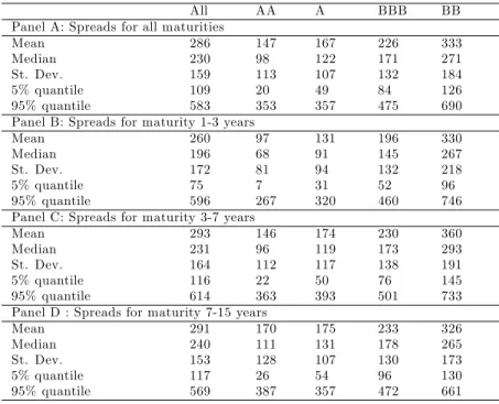
We obtain credit spread curves for AA-rated to BB-rated bonds with maturities ranging from 1 to 15 years. Figure 1 plots these results and Table 3 presents summary statistics.
[Insert Table 3 here]
Across all ratings and maturities, the mean spread is 286 basis points and the median spread is 230 basis points. Relatively high mean and median spreads are due to the sam-ple period selected which includes the recession of 2001 and the residual impact of the 1991 recession –re‡ected in the high level of the credit spread in 1994. Panels A to D present sum-mary statistics for all, short, medium and long maturities, respectively. The term structure of credit spreads for investment grade bonds is upward sloping whereas that for speculative grade bonds is upward sloping for short and medium terms and becomes downward sloping for long terms. Also, credit spread standard deviations are clearly higher for speculative grade bonds across maturities suggesting more variable and unstable yields for this bond group.
8.2 High and low credit spread episodes
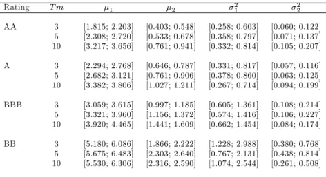
The switching regime model is estimated for each credit spread series separately, with respect to the rating and to the maturity. The parameter estimates b are given in Table 4.
[Insert Table 4 here]
The mean of credit spreads is higher for lower ratings. For investment grade bonds (AA to BBB), the credit spread mean, in both regimes, increases with maturity –consistent with an upward sloping credit spread curve. For speculative grade bonds, the credit spread mean increases until the medium term and then decreases in the long term – consistent with a humped credit spread curve. The credit spread variance, in both regimes, increases as credit ratings decline. It also increases from short to medium term but decreases in the long term. In state 1, the credit spread mean ranges between 2.0% and 4.2% for investment grade bonds and between 5.6% and 8.0% for speculative grade bonds. However, in state 2, the credit spread mean ranges between 0.5% and 1.5% for investment grade bonds and between 2.0% and 4.4% for speculative grade bonds. Thus, across ratings and maturities, the mean of state 1 is always higher than the mean of state 2. The variance of the credit spreads, in state 1, ranges between 0.4% and 1.1% for investment grade bonds and between 2.1% and 3.6% for speculative grade bonds. However, in state 2, the variance ranges between 0% and 0.1% for investment grade bonds and between 0.6% and 1.0% for speculative grade bonds –which is much lower than the credit spread variance in state 1. Overall, these maximum likelihood estimates associate state 1 with a higher credit spread mean and variance. Therefore, we refer to state 1 as a high mean –high volatility regime (high regime) and to state 2 as a low mean –low volatility regime (low regime).
The point estimates of p11 range from 0.943 to 0.989, while the point estimates of p22
range from 0.978 to 0.991. These probabilities indicate that if the system is either in regime 1 or regime 2, it is likely to stay in that regime. Con…dence intervals for the mean and the variance of credit spreads in each regime also support the speci…cation of the regimes. Across ratings and maturities, the mean and the variance of the high regime are statistically di¤erent from those of the low regime at least at the 5% level (Table 5). The only exception is found with the variance of the 5-year BB spreads. We also …nd – results are not reported here – that the unconditional mean and variance of credit spreads in the single regime model are statistically di¤erent from those in the low and high regimes.
[Insert Table 5 here]
Figure 2 plots times series of credit spreads along with the smoothed probabilities p(st=
1jy1; :::; yT; b) indicating the months when the process was in the high regime. The …gure
also shows that for all ratings and maturities the probability that the credit spread is in the high regime at the beginning of the NBER recession (shaded region) is higher than 0.5. One exception is for low grade bonds with short maturities, where the switching happens a few months earlier. The …rst state is also prevalent for most months in 1994.
[Insert Figure 2 here]
All credit spread series stay in the high regime from 2001 to late 2004 although the 2001 recession lasts for only a few months. This indicates that following the systematic shock of 2001, high spread levels are likely to persist in the high regime at least until the announcement date of July 2003. We also notice that high grade spreads (AA and A) do not decrease for many months after the announcement date.
In the reminder of this section, we characterize the credit cycle –with respect to ratings and maturities –using the regime switching structure obtained for credit spreads. To ascer-tain that we are using the correct speci…cation of the credit cycle, we perform the following robustness check (detailed results are available upon request). We regress each credit spread level on the corresponding dummy for the credit cycle. We …nd an adjusted R-squared of about 83% for AA and A spreads and about 80% for BBB and BB.
8.3 Comparative explanatory powers of models
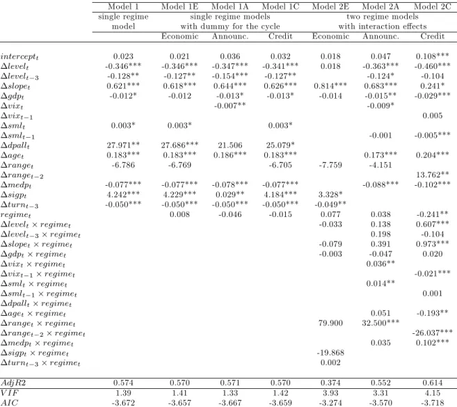
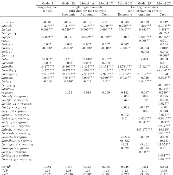
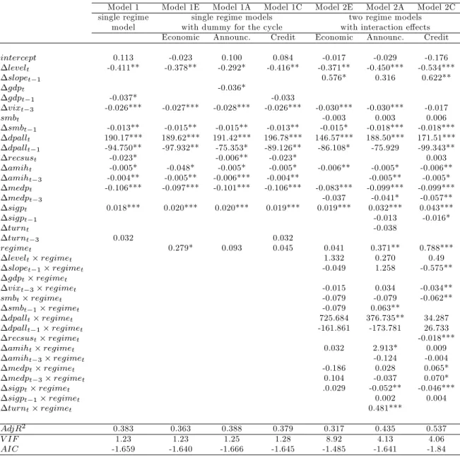
The main result in Collin-Dufresne et al. (2001) is that variables that should theoretically explain credit spread changes have limited explanatory power in the single regime model (no more than an adjusted R-squared of 25%). The analysis of the seven models described in Equations 15 to 21 reveals new insights into the ability of key determinants to explain credit spread di¤erentials. For conciseness, we report only the results for bonds with 10 years to maturity.
[Insert Table 6]
Our results show that the introduction of the regimes in the credit spread dynamics (Model 2C) enhances the explanatory power of theoretical determinants. In particular, the total e¤ect of these determinants throughout the sample period is weakened in the single regime models (Model 1, Model 1E, Model 1A, and Model 1C), thus reducing their explanatory power in most cases. Notice that all these models do not include interaction e¤ects but may include a dummy variable to account for the states in the credit cycle (Model 1C) or the economic cycle (Model 1E and Model 1A). Therefore, the explanatory power of Model 2C is not driven by the addition of the prevailing cycle as an explanatory variable. We also …nd that by conditioning on the states of the economic cycle (Model 2E) we cannot signi…cantly improve the explanatory power of the single regime models. When we condition on the announcement period (Model 2A) we do better than Model 2E but not as good as Model 2C. It appears then that Model 2E does not capture the total e¤ect of the economic recession on credit spreads due to the late announcement and Model 2A does not capture the e¤ective period of recession. Table 6 reports the adjusted R-squared for the seven models considered here. Relative to Model 1, Model 2A and Model 2E, Model 2C has the highest adjusted R-squared. However, relative to Model 1, Model 1E, Model 1A, and Model 1C do not lead to a signi…cant improvement. More interestingly, Model 2C always has the minimum value of AIC along with the highest explanatory power, which reaches on average 60% across all ratings. Detailed results for each of these models are reported in Tables 7 to 10. As can be noted from these tables, the retained sets of explanatory variables in the seven models are di¤erent because the model selection is based on the lowest AIC, in all cases starting from the same initial variables with respect to the multicollinearity issues. Here, the Variance In‡ation Factor (VIF) should not exceed the critical level of 10 for the regression to be retained.10
[Insert Table 7 to Table 10]
To further support our results, we compare the regime-based model (Model 2C) and the single regime model (Model 1) using the same set of explanatory variables. First, we use
1 0
the explanatory variables in Model 2C (Xt;i;m2C ) and derive the single regime model by setting
the coe¢ cients 2C2;i;m = 0 and 2C3;i;m = 0 in Equation 21. In this case, Model 2C and the
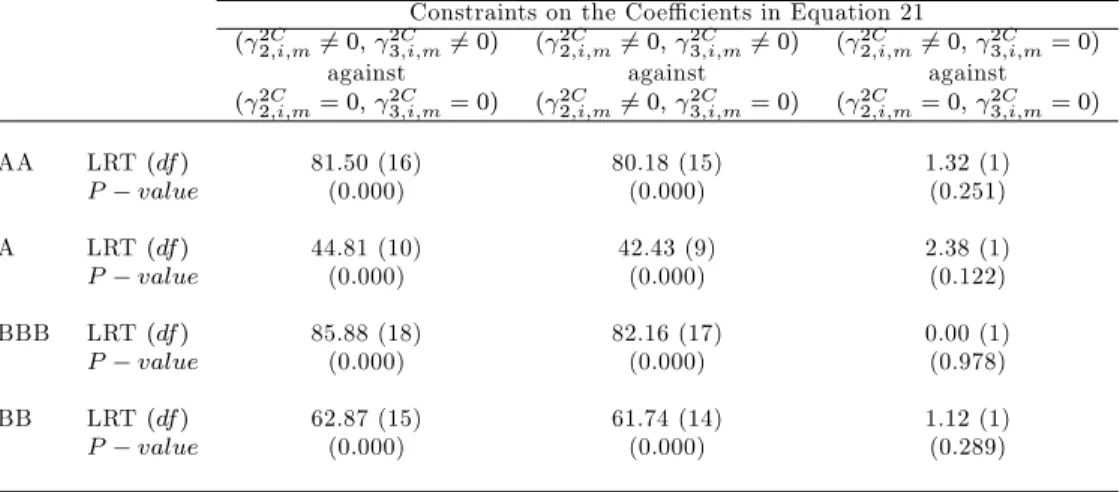
obtained single regime model are nested and can be compared using the Likelihood Ratio Test (LRT). Table 11 shows that, for all ratings, the LRT favors Model 2C. Model 2C also performs better than the single regime model that includes an additional dummy variable for the regimes obtained by setting 2C2;i;m 6= 0 and 2C3;i;m= 0 in Equation 21. In both cases, the Chi2 statistic is always signi…cant at least at the 1% level favoring Model 2C. In addition, when we compare both single regime models obtained from Equation 21 (i. e., 2C2;i;m= 0 and
2C
3;i;m= 0 against 2C2;i;m6= 0 and 2C3;i;m = 0) we …nd that the addition of the dummy variable
for the regimes does not improve the single regime model. Hence, the enhanced explanatory power in Model 2C is driven by the interaction e¤ects. Moreover, omitting interaction e¤ects decreases the adjusted R-squared by roughly 10% for A spreads to up to 30% for AA spreads (Table 12). Table 12 also shows that the addition of the dummy variable for the regimes yields only a marginal positive e¤ect compared with the obtained single regime model. Note that this result holds only for AA and A spreads.
[Insert Table 11 and Table 12 here]
Next, we use the explanatory variables in Model 1 (Xt;i;m1 ) and derive the regime-based
model by adding two terms to Equation 15.
Yt;i;m = 10;i;m + Xt;i;m1 11;i;m+ 12;i;m regimeCt;i;m
+ Xt;i;m1 13;i;m regimeCt;i;m+ 1Ct;i;m; (23)
The …rst term is ( 12;i;m regimeC
t;i;m); which accounts for the regimes in the credit cycle.
The second term is ( Xt;i;m1 13;i;m regimeCt;i;m), which accounts for the interaction e¤ects
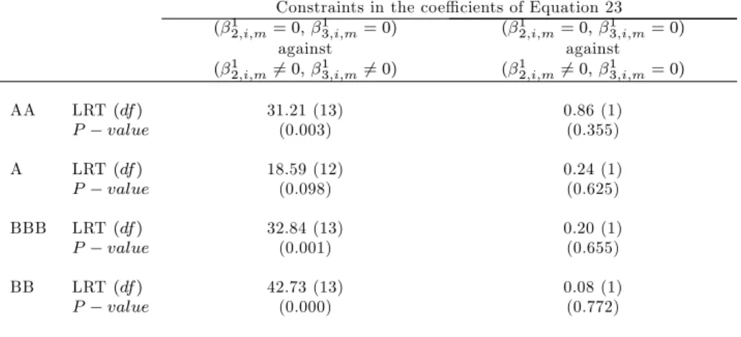
of the explanatory variables in Model 1 with the regimes in the credit cycle. Model 1 and the regime-based model obtained are then nested. Table 13 shows that the LRT always favors the regime-based model obtained due to the addition of interaction terms. The addition of the dummy variable alone does not improve the results even in this case. The corresponding adjusted R-squared are reported in Table 14.
[Insert Table 13 and Table 14 here]
Then, we repeat the analysis by conditioning on the states of the economic cycle. The obtained regime-base model is given by Equation 24.
Yt;i;m = 10;i;m + Xt;i;m1 11;i;m+ 12;i;m regimeEt;i;m
+ Xt;i;m1 13;i;m regimeEt;i;m+ 1Et;i;m; (24)
In this case, conditioning on the states of the economic cycle rather than the credit cycle does not lead to similar results (results, not reported here, are available upon request). The LRT favors always the single regime model ( 12;i;m = 0, 13;i;m = 0 relative to 12;i;m 6= 0,
1
3;i;m6= 0 and 12;i;m6= 0 and 13;i;m = 0 in Equation 24) with the signi…cance level of 1%. In
addition, the single regime model has the highest adjusted R-squared and the lowest AIC. For instance, we contrast Model 2C with Model 2E and Model 2A. Since all models include di¤erent sets of explanatory variables based on model selection criteria we perform two dif-ferent tests.11 Initially, using the same set of explanatory variables as in Model 2C ( X2C
t;i;m),
we condition on the states of the economic cycle (i.e., regimeEt;i;m instead of regimeCt;i;m in
Equation 21) to obtain Model 2E and then we condition on the announcement period (i.e., regimeAt;i;m instead of regimeCt;i;m in Equation 21) to obtain Model 2A. The adjusted
R-squared for all rating classes dropped by about 20% on average in Model 2E and by about 14% on average in Model 2A. The results are reported in Table 15. We also …nd that most of the interaction coe¢ cients are statistically signi…cant with regimeCt;i;m and never
signif-icant with regimeEt;i;m and regimeAt;i;m. Further, across all rating classes, the F-test does
not reject the null hypothesis for all the coe¢ cients of the interaction terms being equal to zero (alpha=1%) when we condition on regimeE
t;i;m and rejects the null hypothesis when we
condition on regimeCt;i;m. When we condition on regimeAt;i;m the F-test only rejects the null
for AA and BBB ratings (Table 16). 1 1
Notice that many variables are dropped from Model 2E (relative to Model 2C) because of collinearity issues. For example, in most cases, the realized default probability, the recovery rate and some illiquidity variables fail the F-test for the regression to be statistically signi…cant. Further, when these variables are included in the interaction terms, the Variance In‡ation Factor (VIF) becomes extremely high because these variables are strongly correlated with the states of the economic cycle.
[Insert Table 15 and Table 16 here]
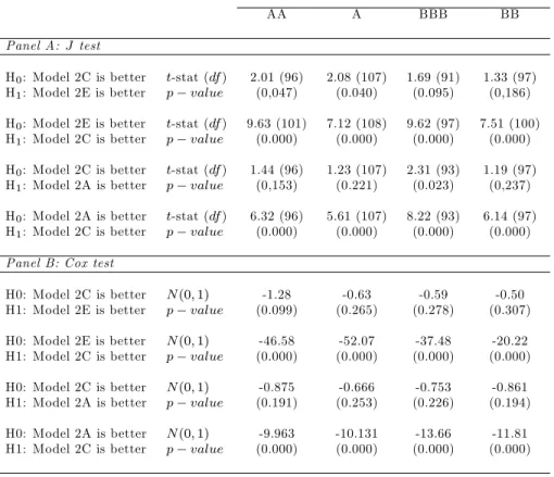
Finally, we contrast the three models directly using the J test (Davidson and MacKinnon, 1981) and the Cox-type test (Cox 1961, 1962; Pesaran 1974; Pesaran and Deaton 1978) for nonnested models. The null hypothesis is performed on both sides. We …rst test whether Model 2C is better than Model 2E or Model 2A, then we test whether Model 2E or Model 2A are better than Model 2C. Both tests favor Model 2C and are statistically signi…cant at the 5% level or higher. One exception applies for the J test where it fails to discriminate between Model 2C and Model 2E for AA and A spreads and between Model 2C and Model 2A for BBB spreads (Table 17).
[Insert Table 17 here]
Overall, relative to the single regime model, our results constantly favor the regime-based model in which the contributions of the explanatory variables are conditioned by the regimes in the credit cycle.
8.4 Determinants in di¤erent regimes
Our results in the single regime model (Model 1) are consistent with the existing literature (Table 7 to Table 10). The level, the slope, the GDP, as well as the Small-Minus-Big and the SML factors are shown to be statistically signi…cant across di¤erent ratings.12 We enhance
the explanatory power of Model 1 by introducing new measures of liquidity which are shown to be very signi…cant across all ratings. The signi…cance level is even stronger for lower grade bonds, as the selected liquidity measures are based on transaction price movements in the bond market. These liquidity measures include the range, median price, price volatility, Amihud measure and turnover. We also …nd that the age has a non negligible e¤ect for high grade bonds. All the variables have the predicted sign, except the CMT slope, which has a positive e¤ect on credit spreads.13
1 2
Since we use portfolios of …xed maturities rather than portfolios of average maturities including short, medium and long term bonds, di¤erent ratings and maturities are found to be a¤ected by di¤erent variables and lags.
1 3
We …nd that changes in the CMT slope and changes in credit spreads are positively correlated. The correlation coe¢ cient is 0.43 on average across ratings. In terms of levels, this coe¢ cient is even stronger (0.92).
Previous results show that Model 1 has limited explanatory power because it assumes that the explanatory variables have the same e¤ect on credit spreads over distinct regimes. We also show that Model 2C is our best performing model (Table 11 to Table 17). Thus, we base our comments on the results obtained with Model 2C. Across ratings, the CMT level and slope are shown to be statistically signi…cant in both regimes, while the e¤ect of the slope is stronger in the high regime. Like the slope, the liquidity variables are found to be signi…cant in both regimes but their signi…cance is greater in the high regime, especially for low grade bonds. The age and the GDP are important only for AA and A spreads. Their contribution, while marginal, is stronger in the low regime. The SMB and the SML also make a marginal contribution in the high regime.
We now focus on the coe¢ cient signs of di¤erent variables in di¤erent regimes. In partic-ular, most of the signs in the low regime are inverted in the high regime, thus weakening their total e¤ect in the single regime model. We summarize these signs in Table 18. As can be seen in this table, the signs of the explanatory variables in the single regime model (Model 1) are, in most cases, the same as those in the low regime for Model 2C. However, except for the variables that are found to be closely related to the behavior of credit spreads (like the age, the CMT slope, and the realized default probability), all the other variables have an inverted sign in the high regime. These variables include most of the market factors and liquidity factors as well as the recovery rate. All these variables are likely to react to macroeconomic conditions well before credit spreads do. Actually, the NBER reports that after an economic recession its committee usually waits to declare the end of the recession until it is con…dent that any future downturn in the economy would be considered a new recession and not a continuation of the preceding recession. Thus due to the late NBER announcement, these variables are expanding well before the end of the high credit spread regime. It follows that after the economic recession, the sign e¤ects are inverted especially for spreads with high grades and long maturities. These spreads are also slower to adjust to any new economic state. Model 2E fails to capture these inverted signs. That is why the explanatory power of the single regime model does not improve when we condition on the economic cycle. On the other hand, Model 2A does better than Model 2E because it captures most of the sign
patterns. However, Model 2A does not capture the e¤ective recession since the recession is always announced later on. Therefore, Model 2C performs best since it captures both the economic recession and the announcement period. The regimes in Model 2C also take into account the di¤erent patterns accross di¤erent ratings and maturities while the economic cycle and the announcement period are …xed across all spreads. As shown in Figure 2, the high regime in low grade bonds starts before the economic recession and ends also before the high regime of high grade bonds.
[Insert Table 18 here]
To better explain the pattern of the inverted signs for some variables in the high regime, we discuss the case of the CMT level. Across all ratings, Table 18 shows that the level has a negative sign in the low regime. However, in the high regime, this coe¢ cient turns out to be positive and statistically signi…cant for AA and A spreads. For example, for A spreads, the coe¢ cient of the level is -0.460 in the low regime and becomes +0.147 in the high regime. Both coe¢ cients are signi…cant at least at the 5% level. Figure 3 plots AA-rated to BB-rated credit spreads with 10 remaining years to maturity along with the CMT level. As shown in this …gure, outside the high regime, the relation between the CMT level and credit spreads appears negative. As a matter of fact, the correlation between both series ouside the high regime is negative –consistent with the theoretical settings of Merton (1974), Longsta¤ and Schwartz (1995) and Du¤ee (1998). However, in the high regime the negative relation often disappears and the correlation between both series is found positive. Inside the shaded region (2001 recession), credit spreads are increasing and risk-free rates are decreasing. Then, between the end of the recession (November 2001) and the announcement of the end (July 2003), credit spreads and risk-free rates are often moving on the same direction. After the announcement of the recession end, the negative relation is clearly re-established. When the whole sample period contains one or more recessions, then the total e¤ect of risk-free rates on credit spreads can be dominated by the high regime and the relation appears positive overall. This result can explain why in previous empirical works like those of Morris, Neale, and Rolph (1998), and Bevan and Garzarelli (2000) the relation between risk-free rates and credit
spreads was found positive. The same pattern for the CMT level is observed for the VIX, the SMB, the SML, the recovery rate, and the illiquidity factors based on bond transaction prices.
[Insert Figure 3 here]
In contrast, the CMT slope, the bond age and the realized default probability have the same signs in both regimes. For example, for A-rated bonds, the coe¢ cient of the month t slope in the low regime is +0.241 and is statistically signi…cant at the 10% level. In the high regime, this coe¢ cient increases to 0.973 and is statistically signi…cant at the 1% level. Similar to the slope, the realized default probability and the age have positive signs in both regimes, but for the age the e¤ect is weaker in the high regime. For A spreads, the coe¢ cient of the age is +0.204 in the low regime and is signi…cant at the 1% level, while in the high regime its e¤ect signi…cantly decreases to +0.11.
The evidence for the GDP is weaker because its coe¢ cient in the high regime is not statistically signi…cant. However, for AA to BBB spreads, the GDP is statistically signi…cant at least at the 5% with the predicted sign in the low regime. Moreover, for AA to BBB spreads, the F-test rejects the null hypothesis for the coe¢ cient of the GDP to be equal to zero in the low regime and accepts the null for the coe¢ cient to be equal to zero in the high regime. The F-test is signi…cant at least at the 5% level. This further suggests that the economic cycle is di¤erent from the prevailing credit cycle. Thus, macroeconomic fundamentals may not capture total state-dependent movements in the credit spread dynamics.
For a last check, we analyzed each set of factors (market, default, liquidity) separately (results available upon request). This was done to test whether the inverted signs in the high regime are due solely to the correlation between di¤erent sets of factors considered in Model 2C. Variables included in each set of factors are also selected based on the lowest AIC. The results obtained with each set of factors –across ratings –are similar to those obtained with Model 2C. Thus, we still observe the sign inversions in the high regime. Further, for each factor model we contrast the single regime model to the regime-based model. Based on the LRT, we still favor the regime-based models which are similar to Model 2C but include market, liquidity or default factors (Table 19).
[Insert Table 19 here]
9
Conclusion
The main contribution of this study is to examine the impact of modeling the credit cycle endogenously on credit spread determinants. The credit cycle is derived from the switching regime structure for credit spreads. The obtained credit cycle and the NBER economic cycle exhibit di¤erent patterns.
Even though credit spreads are counter-cyclical, their high level following a systematic shock in the economy is triggered by an announcement e¤ect and a persistence e¤ect. These two e¤ects produce a credit cycle that is much longer than the economic cycle. In particular, the NBER waits for a certain time before announcing the beginning and the end of a recession. It follows that, following the GDP, many credit spread determinants may adjust to the period of expansion well before credit spreads do. In the meantime, the coe¢ cient signs of several determinants are often inverted in the high regime. These changes in the coe¢ cient signs are hidden in the single regime model leading to limited total e¤ects and thus reducing the explanatory power of the model. Our results thus o¤er new insights into the existing models in the credit risk literature using regime switches derived from macroeconomic fundamentals. Our results suggest that by conditioning on credit spread regimes we enhance the ex-planatory power of the single regime model. Moreover, we show that the single regime model cannot be improved by conditioning on the states of the economic cycle or on the announce-ment period of the NBER cycle. In particular, most of the interaction terms in the regime based model are almost never signi…cant when considering the states of the economic cycle, whereas they are highly signi…cant when we consider the credit cycle.
Moreover, our results show that di¤erent factors have di¤erent contributions in distinct credit spread regimes. This further suggests that the regime-based model also enhances the explanatory power of key determinants. The factors considered generate up to 60% of the variation in credit spread changes. Finally, our study is a further step to help solve the credit spread puzzle documented in recent research.
References
[1] Alexander, C., and Kaeck, A. (2007), "Regime Dependent Determinants of Credit De-fault Swap Spreads", Journal of Banking and Finance, 32, 1008-1021.
[2] Altman, E., and Kishore, V. (1996), "Almost Everything You Wanted to Know about Recoveries on Defaulted Bonds", Financial Analysts Journal, 52, 57-64.
[3] Altman, E., Brady, B., Resti, A., and Sironi, A. (2005), "The Link between Default and Recovery Rates: Theory, Empirical Evidence, And Implications", Journal of Business, 78, 2203-2228.
[4] Altman, E., Resti, A., and Sironi, A. (2001), "Analyzing and Explaining Default Recov-ery Rates", International Swaps Dealers Association (ISDA), London.
[5] Amato, J. D., and Remolona, E. M. (2003), "The Credit Spread Puzzle", The BIS Quarterly Review, 22, 51-64.
[6] Amihud, Y. (2002), "Illiquidity and Stock Returns: Cross-Section and Time-Series Ef-fects", Journal of Financial Markets, 5, 31-56.
[7] Bedendo, M., Cathcart, L., and El-Jahel, L. (2004), "The Shape of the Term Structure of Credit Spreads: An Empirical Investigation", Working Paper, Imperial College London, Tanaka Business School.
[8] Bevan, A., and Garzarelli, F. (2000), "Corporate Bond Spreads and the Business Cycle", Journal of Fixed Income, 9, 8-18.
[9] Bhamra, H. S., Kuehn, L. A., and Strebulaev, I. A. (2007), "The Levered Equity Risk Premium and Credit Spreads: A Uni…ed Framework", Working Paper, University of British Columbia and Stanford.
[10] Campbell, J., and Taksler, B. (2003), "Equity Volatility and Corporate Bond Yields", Journal of Finance, 58, 2321-2350.
[11] Chakravarty, S., and Sarkar, A. (1999), "Liquidity in U.S. Fixed Income Markets: A Comparison of the Bid-Ask Spread in Corporate, Government and Municipal Bond Mar-kets", Federal Reserve Bank of New York, Sta¤ Report, 73.
[12] Chen, H. (2008), "Macroeconomic Conditions and the Puzzles of Credit Spreads and Capital Structure", Working Paper, Massachusetts Institute of Technology.
[13] Chen, N. F. (1991), "Financial Investment Opportunities and the Macroeconomy", Jour-nal of Finance, 46, 529-554.
[14] Collin-Dufresne, P., Goldstein, R. S., and Martin, J. S. (2001), "The Determinants of Credit Spread Changes", Journal of Finance, 56, 2177-2208.
[15] Cox, D. R. (1961), "Tests of Separate Families of Hypotheses", Proceedings of the Fourth Berkeley Symposium on Mathematical Statistics and Probability, 1, 105-123.
[16] Cox, D. R. (1962), "Further Results on Tests of Separate Families of Hypotheses", Journal of the Royal Statististical Society Series B, 24, 406-424.
[17] David, A. (2008), "In‡ation Uncertainty, Asset Valuations, and the Credit Spreads Puz-zle", Review of Financial Studies, Forthcoming.
[18] Davidson, R., and MacKinnon, J. G. (1981), "Several Tests for Model Speci…cation in the Presence of Alternative Hypotheses", Econometrica, 49, 781-793.
[19] Davies, A. (2004), "Credit Spread Modelling with Regime Switching Techniques", Jour-nal of Fixed Income, 14, 36-48.
[20] Davies, A. (2007), "Credit Spread Determinants: An 85 Year Perspective", Journal of Financial Markets, 11, 180-197.
[21] Davydenko, S. A., and Strebulaev, I. A. (2004), "Strategic Actions and Credit Spreads: An Empirical Investigation", Journal of Finance, 62, 2633-2671.
[22] Delianedis, G., and Geske, R. (2001), "The Components of Corporate Credit Spreads: Default, Recovery, Taxes, Jumps, Liquidity, and Market Factors ", Working Paper, The Anderson School at UCLA, N 22-01 .
[23] Dempster, A. P., Laird, N. M., and Rubin, D. B. (1977), "Maximum Likelihood from Incomplete Data via the EM Algorithm", Journal of the Royal Statistical Society, 39, 1-38.
[24] Dionne, G., François, P., and Maalaoui, O. (2008), "Detecting Regime Shifts in Corpo-rate Credit Spreads", Working Paper, HEC Montreal.
[25] Downing, C., Underwood, S., and Xing, Y. (2005), "Is Liquidity Risk Priced in the Corporate Bond Market?", Working Paper, Rice University.
[26] Driessen, J. (2003), "Is Default Event Risk Priced in Corporate Bonds?", University of Amsterdam.
[27] Du¤ee, G. (1998), "The Relation between Treasury Yields and Corporate Bond Yield Spreads", Journal of Finance, 53, 2225-2241.
[28] Elton, E. J., Gruber, M. J., Agrawal, D., and Mann, C. (2001), "Explaining the Rate Spread on Corporate Bonds", Journal of Finance, 56, 247-277.
[29] Engle, C., and Hamilton, J. D. (1990), "Long Swings in the Dollar: Are They in the Data and Do Markets Know It?", American Economic Review, 80, 689-713.
[30] Fama, E. F., and French, K. (1989), "Business Conditions and Expected Returns on Stocks and Bonds", Journal of Financial Economics, 25, 23-49.
[31] Goldstein, M., Hotchkiss, E. S., and Sirri, E. R. (2006), "Transparency and Liquidity: A Controlled Experiment on Corporate Bonds", Review of Financial Studies, 20, 235-273. [32] Gorton, G. B., and He, P. (2003), "Bank Credit Cycles," Working Paper, University of
Pennsylvania.
[33] Griep, C. (2002), "Higher Ratings Linked to Stronger Recoveries", Special Report, Stan-dard and Poor’s.