Arithmetic of values of L-functions and generalized multiple zeta values over number fields

(1)

HAL Id: tel-02303034

https://tel.archives-ouvertes.fr/tel-02303034

Submitted on 2 Oct 2019

HAL is a multi-disciplinary open access

archive for the deposit and dissemination of sci-entific research documents, whether they are pub-lished or not. The documents may come from teaching and research institutions in France or abroad, or from public or private research centers.

L’archive ouverte pluridisciplinaire HAL, est destinée au dépôt et à la diffusion de documents scientifiques de niveau recherche, publiés ou non, émanant des établissements d’enseignement et de recherche français ou étrangers, des laboratoires publics ou privés.

Arithmetic of values of L-functions and generalized

multiple zeta values over number fields

Xiaohua Ai

To cite this version:

Xiaohua Ai. Arithmetic of values of L-functions and generalized multiple zeta values over number fields. General Mathematics [math.GM]. Université Pierre et Marie Curie - Paris VI, 2017. English. �NNT : 2017PA066394�. �tel-02303034�

(2)

ARITHMETIC OF VALUES OF L-FUNCTIONS AND

GENERALIZED MULTIPLE ZETA VALUES OVER NUMBER

FIELDS

XIAOHUA AI

INSTITUT DE MATHEMATIQUES DE JUSSIEU-PARIS RIVE GAUCHE (IMJ-PRG)

UNIVERSITE PIERRE ET MARIE CURIE (PARIS 6)

(3)

Contents Contents

1 Introduction

The principal objective of this thesis is to generalize multiple Zeta values to the case when the ground field Q is replaced by an arbitrary number field. The motivation behind the construc-tion comes from the work of A. Goncharov on Hodge correlators and the plectic philosophy of J. Nekov´a˘r and A. Scholl.

We start by constructing the higher plectic Green functions. Hecke once proved that the integral of the restriction of a suitable Eisenstein series over Q to the idele class group of a given number field multipled an idele class character of finite order is equal to the L-functions of this charator. By replacing Eisenstein seris with our higher plectic Green functions, a similar integration gives new results, which give the generalization of classical multiple zeta values and multiple polyloarithms.

According to the plectic principle, a non-trivial subgroup of the ring of integers of a given number field plays an essential role in this work.

1.1 Generalizations of classical Zeta Values

Classically, multiple Zeta values(MZVs) are the periods of mixed Tate motives, namely the MZVs are iterated integrals on P1∖ {0,1,∞}. Mixed motives and their realizations related to classical modular forms were studied by various mathematicians (Beilinson, Beilinson-Levin, Manin, Gon-charov, F. Brown, ...) Moreover, there exist mysterious modular phenomena in the ring of MZVs related to the depth filtration. A good geometric understanding of these phenomena seems that we should put MZVs and modular forms for SL2(Z) in a common framework. Recently, F. Brown

proposed so-called multiple modular values and mixed modular motives.

On the other hand, A. Goncharov used ideas from quantum physics on Hodge theoretical setting to construct so-called Hodge correlators, which provide a new method to describe the corresponding variations of real mixed Hodge structures and a new way to understand periods of motives. He proved that classical polylogarithms, elliptic polylogarithms and their generalizations are all Hodge correlators.

However, all the work mentioned above is built up over the rational field Q. What the situation will be if Q is replaced by an arbitary number field K is still largely open. One natural but non-trivial question is

Question 1.1 How should we define multiple Zeta values over arbitary number fields? What should we put in the missing place in the following diagram to complete this diagram?

Classical zeta values/Q > (partial)Dedekind zeta functions/K

Mutiple zeta values∨ /Q ...>

?

∨...

In this thesis, we propose a potential method to answer this question, inspired by A. Goncharov’s theory on Hodge correlators [10] and by the plectic principle due to J. Nekov´a˘r and A. Scholl [13]. The starting point is to generalize the Hecke formula.

1.2 Hecke’s Formula

Hecke [12] proved that the integral of the restriction of a suitable Eisenstein series over Q to the idele class group of a given number field multipled by an idele class characterχ of finite order is

(6)

1.2 Hecke’s Formula Introduction

equal to the L-functions ofχ, up to some Γ factors. In fact, Hecke’s formula is one of the typical examples within the theory of automorphic periods.

More precisely, Let K be a number field of degree[K ∶ Q] = r1+2r2.

KR= K ⊗RÐ→ R∼ r1×Cr2.

Define the norm map

N= NK/Q⊗id ∶ KR×Ð→ R×.

In order to state Hecke’s formula, we will need the following data: (1) Let U⊂ O×_K,₊be a subgroup of finite index, where

O_K,×₊= O×_K∩(K_R×)₊, (K_R×)₊= (R×₊)r1×(C×)r2. (2) Let I⊂ K be a fractional OK-ideal.

(3)∃ m ∈ N∖{0}, φ ∶ I/mI Ð→ C be a function such that

∀ε ∈ U, ∀α ∈ I ∖{0}, φ(εα) = φ(α). We consider the following embedding (defined up to a conjugation)

GLK(1) ↪ GLQ([K ∶ Q]).

Let E(g,s,φ) be the Eisenstein series defined by

E(g,s,φ) = ∑

x∈I∖{0}

φ(x) ∥g⋅x∥s,

where g∈ GLZ(I)(R) ≅ GL[K∶Q](R) and ∥⋅∥ is a scalar product on KR.

Hecke proved the following formula. [12] ∫_U

R/U

E(u,s,φ) d×µ(u) = C(r1,r2,s,d×µ(u))⎛

⎝ ∑x∈I∖{0} φ(x) ∣NK/Q(x)∣s/[K∶Q] ⎞ ⎠, where UR= Ker(NK/Q⊗1 ∶(KR×)+Ð→ R × +),

and C(r1,r2,s,d×µ(u)) is some Γ factor and d×µ(u) is a Haar measure. In fact we can also make

the formulation in an adelic setting.

In a more concrete setting, we can rewrite Hecke’s formula as follows. Theorem 1.2 (Hecke’s Formula)

∫_U R/U ⎛ ⎝ ∑α∈I∖{0} φ(α) ∥uα∥[K∶Q]s ⎞ ⎠ d×µ(u) = 2πr2 [K ∶ Q]2r1 Γ(s/2)r1Γ(s)r2 Γ([K ∶ Q]s/2) α∈(I∖{0})/U∑ φ(α) ∣ NK/Q(α) ∣s .

One of the objectives of this thesis is to try to generalize this formula in order to produce suitable “secondary”arithmetic objects. First of all we would like to precise the meaning of “secondary”.

The generalization of Hecke’s formula begins with replacing the Eisenstein series by some non-trivial objects, namely so-called higher plectic Green functions, which depend on one basic plectic Green function gν_I(x,u) (Definition 4.1) and on some combinatorial data. We will give the details about the construction of higher plectic Green functions in the fourth and fifth chapters.

Now it is natural to ask

(7)

1.3 Inspiration Introduction

Question 1.3 What are we going to obtain if we integrate these new objects over UR/U ?

This thesis will answer this question. We would like to give the simplest example by integrating the basic plectic Green function.

Theorem 1.4 (Reinterpretation of Hecke’s formula) Let F be a totally real field of degree r= [F ∶ Q] and D the different ideal of F. If I is a fractional ideal of F, let

I∗= {x ∈ F ∣ Tr(xI) ⊂ Z} = D−1I−1.

If x∈ FR= F ⊗R, if U ⊂ O×F,+a subgroup of finite index and if∀ε ∈U, (ε −1)⋅x ∈ I, which is equivalent

to

xI∈ (FR/I)U,

and ifν ∶ Hom(F,R) Ð→ {0,1}, consider

gν_I(x,u) = lim η→0+ ∑ n∈(I∗_∖{0})/U sgn(n)νe 2πiTr(nx) ∥un∥r+η ,

where u∈ UR= Ker(N ∶ (FR×)₊Ð→ R×+) and ∥⋅∥ is the standard scalar product on FR≅ Rr.

∀_ε∈ U, gν_I(x,εu) = gν_I(x,u).

By integration in a similar way as Hecke did, we obtain

∫_U R/U gν_I(x,u)du =2 r−1_Γ(1/2)r Γ(r/2) η→0lim+ ∑ n∈(I∗_∖{0}/U) sgn(n)ν e 2πiTr(nx) ∏r j=1∣nj∣(r+η)/r . Note that N(n) = N_F_/Q(n) = r ∏ j=1 nj, hence ∫_U R/U gν_I(x,u)du =2 1−r_Γ(1/2)r rΓ(r/2) η→0lim+ ∑ n∈(I∗_∖{0})/U sgn(n)ν e 2πiTr(nx) ∣N(n)∣(r+η)/r.

It is easy to see that we recover the Hecke formula, the righthand side is a linear combination of special values L(1,χF) for certain Dirichlet characters χF of F of signatureν.

For other more complicated higher plectic Green functions, the results are highly non-trivial, some non-trivial iterated integrals make their appeareance in a subtle way. However, if the number field K is just the rational field Q, the integration_∫_U

R/U is trivial and we prove that the higher plectic Green

functions deliver linear combinations of classical zeta values.

1.3 Inspiration

Before giving our main results, we will fist talk about two sources of inspiration of our construction in the next section and give some simple examples in order to illustrate our strategy.

(8)

1.3 Inspiration Introduction

1.3.1 Goncharov’s Hodge correlators

In A. Goncharov’s recent work [10], he constructed so-called Hodge correlators from just one fun-damental object, namely the Green function, and certain Feynman diagrams, as in perturbative quantum field theory. In fact, the Green function contributes as the propagator which in Feynman diagrams serves to calculate the rate of collisions in quantum field theory.

Goncharov introduced such an idea to a Hodge-theoretic setting. He discovered that the so-called Hodge correlators are the coefficients of twistor connections, which describe the correspond-ing variations of real mixed Hodge structures. He proved that classical polylogarithms, elliptic polylogarithms and their generalizations are all Hodge correlators.

For example, over C×, the Green function G(x,y) is log∣x−y∣2. Applying a non-trivial integral formula of Levin, Goncharov proved that the usual polylog can be writen as a Hodge correlator. Based on such a construction, he obtained higher multipolylogarithms, more precisely, he proved that the generating series of cycle multiple polylogarithms is a Hodge correlator, with the generating series of classical polylogarithms serving as a Green function. His construction of Hodge correlators on C× gives a variant of multiple polylogs, but a precise relation to the classical definition is not made explicit.

1.3.2 Plectic Philosophy

Over a totally real field F, J. Nekov´a˘r and A. Scholl [13] formulated what they call the plectic conjecture. The geometric objects in this conjecture are Shimura varities/stacks whose definition groups are restrictions of scalars from an algebraic group over F. More concretely, they work with abelian varieties with real multiplication by OF, where OF is the ring of integers of F. We will try

to explain the plectic principle in the following.

If B is a connected complex manifold. Let X/B be a family of abelian varities with real mul-tiplication, and s∶ B Ð→ X a nonzero torsion section fixed by a subgroup of finite index U ⊂ O×_F,₊. This subgroup U acts naturally on X and acts trivally on B, then we should consider the following diagram

X×UEU >X

B×UEU

∨ π

>B,∨

where EU is the total space over the classifying space BU of the group U and B×UEU= B×EU/U.

When B= {pt} , then X is a variety, we have the following situation

X×UEU

BU.∨

Nekov´a˘r and Scholl [13] constructed in their work a U -equivariant current ˜θ on ˜X= X ×UR, where

UR= EU. In fact ˜θ is a plectic generalisation of the (slightly modified) log∣θ(τ,z)∣ of the absolute

value of the standard Theta function on the elliptic curve E= C/Zτ +Z, which is the Green function on E.

So s∗( ˜θ) is U-equivariant on ˜B = B×UR. Then s∗( ˜θ) can descend to a current on B×UR/U,

and we can compute the trace

π∗(s∗( ˜θ)) = ∫

UR/U

s∗( ˜θ),

(9)

1.4 Main results Introduction

which gives very interesting functions, such as generalized Eisenstein-Kronecker-Lerch series. The above integral, as well as its variants involving more complicated functions than ˜θ , can be computed by integrating suitable expressions depending on∥ux∥ over UR. For this purpose, the

Hecke transform is introduced and used in their work. Here is a typical example.

Proposition 1.5 (Hecke transform)[14]

Let UR⊂ (R×+)rbe the subgroup

UR= {(uj)∣∏uj= 1}

with the measured×u=du1_u1 ∧⋯∧dur−1

ur−1. Let∣∣⋅∣∣ be the Euclidean norm on C

r_{, on which U acts by}

multiplication. Let(pj) ∈ Zr, p= ∑ pj. Then for any x∈ (C×)rand s∈ C with Re(s) > 0,

∫_U R ∣∣ux∣∣−2s_∏ j u−2pj j d ×_u₌ 2r−1 Γ(s) ∏j Γ(p + s r −_p_j)∣x_j∣2(pj−(p+s)/r)_. 1.4 Main results

In our work, we consider a generalisation of log∣1−e2πix∣2on the compact real torus

S1= {e2πix∣x ∈ R/Z} ⊂ C×.

This function is the restriction of the Green function G(1,y) = log∣1−y∣2of the origin of C×to S1. We are going to consider corresponding objects on tori with real multiplication.

Let F be a totally real field of degree r= [F ∶ Q], we have the trace map Tr = Tr_F_/Qand the norm map N= NF/Q. Let D be the different and let I be a fractional ideal of F and

I∗= {a ∈ F ∣ Tr(aI) ∈ Z} = D−1I−1.

Let∣∣ ⋅ ∣∣∶ FR= F ⊗RÐ→ R∼ Hom(F,R)Ð→ R+∪{0} be the standard euclidean norm. As above, let

UR= Ker(N ∶ (FR×)+Ð→ R×+) = {(u1, . . . ,ur) ∈ Rr+∣ u1⋯ur= 1}.

Then we can define the “plectic” Green function associated to the ideal I Definition 1.6 (Plectic Green function)

gI(x,u) = lim

η→0+ ∑ n∈I∗_/{0}

e2πiTr(nx)

∣∣un∣∣r+η , x∈ FR/I, u ∈ UR,

which can also be defined as∑n∈I∗_∖{0}e 2πiTr(nx)

∣∣un∣∣r , viewed as a distribution on(FR/I)×UR.

We can also add an additional choice of multisignsν∈ {0,1}Hom(F,R). Then the modified “plectic” Green function becomes

gν_I(x,u) = lim η→0+ ∑ n∈I∗_/{0} sgn(n)νe 2πiTr(nx) ∣∣un∣∣r+η , x∈ FR/I, u ∈ UR.

There is also a second method to add a multisign

gI,ν(x,u) = lim η→0+ ∑ n∈I∗_/{0} sgn(n)=(−1)ν e2πiTr(nx) ∣∣un∣∣r+η , x∈ FR/I, u ∈ UR. 7

(10)

(11)

1.4 Main results Introduction

Remark 1.10 We can also add multisigns here, there are two methods. The first way is to associate

each edge a multisignνe= (νe1, . . . ,νer), then the formula in 4.9 will then contain terms sgn(ne)ν(e):

Gν

I,Γ(k),S({xv}v∈S,u) = vol(FR/I)∣V (Γ)/S∣+∣k∣−∣E(Γ)∣_{δ →0}lim+∑

′

{n,c(n)∈H1(Γ,S)⊗I∗}sgn(ne)

ν(e) e2πiTr(∑v∈S(∂ n)vxv)

∏e∈E(Γ)∣∣une∣∣ke(r+δ )

.

The second method to add mutisigns by taking into account the ne∈ I∗∖{0}, such that sgn(ne) =

(−1)νe_{for a given multisign}_ν

eto each edge e. Then

G_I,_ν,Γ(k),S({x_v}_v_∈S,u) = vol(FR/I)∣V (Γ)/S∣+∣k∣−∣E(Γ)∣ lim δ →0+∑ ′ {n,c(n)∈H1(Γ,S)⊗I∗} sgn(ne)=(−1)ν(e) e2πiTr(∑v∈S(∂ n)vxv) ∏e∈E(Γ)∣∣une∣∣ke(r+δ ) .

In fact, we usually prefer the second definition G_I,_ν,Γ(k),S({xv}v∈S,u).

Similarly, we can generalize the definition of plectic Green functions to any number field. Definition 1.11 (Plectic Green functions for arbitary number fields)

Let K be a number field with r1real places(vi)1≤i≤r1 and r2complex places(wj)1≤ j≤r2and of degree

[K ∶ Q] = r1+2r2. We have the trace mapTr= TrK/Q

KR≅ Rr1×Cr2

and we have a Hermitian product

⟨ ∣ ⟩ ∶ KR×KRÐ→ C ⟨(xv,zw)∣(x′v,z′w)⟩ = ∑ v xvx′v+∑ w zwz′w, where x= (xv,zw). Let ∥⋅∥ = ⟨⋅∣⋅⟩1/2 ,

then the plectic Green function can be defined as gI(x,u) = ∑

n∈I∗_/{0}

e2πiTr(nx)

∣∣un∣∣r1+2r2, x∈ KR/I, u ∈ UR,

which is a distribution on(KR/I)×UR.

1.4.1 Generalized MZV for totally real fields

If we suppose that there exists a subgroup U⊂ O×_F,₊of finite index stabilising{xv} for each v ∈ S, we

can apply the Hecke transform to define a new function as follows. Definition 1.12

F_I,_Γ,S({x_v}_v∈S) = (O×_F,₊∶_U)−1_∫

UR/U

G_I,_Γ,S({x_v}_v∈S,u)d×u, where d×u=du1⋯dur−1

u1⋯ur−1 ,∏ r

j=1uj= 1 and UR/U = BU ≅ (S)r−1is the classifying space of U ≅ Zr−1.

(12)

(13)

1.4 Main results Introduction G_I,_ν,Γ 1,∂ Γ1({xv}v∈∂ Γ1,1) = ∑ n1+n2+n3=0,ni∈Z∖{0} sgn(ni)=(−1)νi e2πi(n1xv1+n2xv2+n3xv3) ∣n1∣σ1∣n2∣σ2∣n3∣σ3 , whereν1= ν2= 0, ν3= 1. Then Z_I,_ν(Γ₁_,_{∂ Γ}₁) = ∑ n1+n2+n3=0,ni∈_Z∖{0} sgn(ni)=(−1)νi 1 ∣n1∣σ1∣n2∣σ2∣n3∣σ3 =_n1_,_n2∑∈_N∖{0} 1 ∣n1∣σ1∣n2∣σ2∣n1+n2∣σ3 Z_I,_ν(Γ₁,∂ Γ1) = ∑ n1,n2∈N∖{0} 1 nσ1 1 n σ2 2 (n1+n2)σ3 .

We show in Example 4.22 that

Z_I,_ν(Γ₁,∂ Γ₁) = ∑ r+s=σ1+σ2 (Cσ1−1 r−1 +C σ2−1 r−1 )ζ(s,r +σ3).

Hereζ(s,r+σ3) is a classical double zeta value of weight r+s+σ3= σ1+σ2+σ3, which means that

Z_I,_ν(Γ₁,∂ Γ1) can be expressed as a Z-linear combination of double zeta values of this weight.

1.4.3 The case of a general totally real field

If[F ∶ Q] = r > 1, then the generalized multiple zeta value ZI(Γ,S) is highly non-trivial.

Let us see the case of r= 2, we have the following theorem Theorem 1.17 Given k= (k1, . . . ,kd) and ∣k∣ = k1+...+kd.

(1)If2∤ ∣k∣, then after several differentiation with respect to the coefficients αj,βj, the essential part

of the definition of higher plectic Green function I2(d,k) = ∫ ∞ 0 1 ∏d j=1(α2ju+β2ju−1)kj d×u

can be written as product ofπ and an element of Q(α1, . . . ,αd,β1, . . . ,βd).

(2) If2 divides∣k∣, then I2(d,k) can be written as

d ∑ j=1 γj⋅log( βj αj), whereγj∈ Q(α₁2, . . . ,α_d2,β₁2, . . . ,β_d2).

Example 1.18 Consider the case d= 3, m = 0 and n = 1. Then

I(αj,βj) = ∫ ∞ 0 1 ∏3 j=1(α2ju +βj2u−1) du u = −π₂∑3 j=1 αjβj ∏3 k=1,k≠ j∆k j= − π 2( α1β1 ∆12∆13 − α2β2 ∆21∆23 + α3β3 ∆12∆23) = π 2(α1β2+α2β1)(α1β3+α3β1)(α2β3+α3β2) . 11

(14)

(15)

Goncharov’s Theory of Hodge correlators

2 Goncharov’s Theory of Hodge correlators

In this section, we will explain the idea of A. Goncharov’s theory of Hodge correlators, where we are inspirated for the construction. This theory provides a new point of view of periods. Our explanation is based on several simple examples.

2.1 Introduction

In Goncharov’s recent work [10], he constructed so-called Hodge correlators from just one fun-damental object, namely the Green function, and certain Feynman diagrams, as in perturbative quantum field theory. In fact, the Green function contributes as the propagator which in Feynman diagrams serves to calculate the rate of collisions in quantum field theory.

Goncharov introduced such an idea to a Hodge-theoretic setting. He discovered that the so-called Hodge correlators are the coefficients of twistor connections, which describe the correspond-ing variations of real mixed Hodge structures. He proved that classical polylogarithms, elliptic polylogarithms and their generalizations are all Hodge correlators.

For example, over C×, the Green function G(x,y) is log∣x − y∣2. Applying a non-trivial inte-gral formula of Levin, Goncharov proved that the usual polylogarithm can be writen as a Hodge correlator. Based on such a construction, he obtained higher multipolylogarithms, more precisely, he proved that the generating series of cycle multiple polylogarithms is a Hodge correlator, with the generating series of classical polylogarithms serving as a Green function. His construction of Hodge correlators on C×gives a variant of multiple polylogs, but a precise relation to the classical definition is not made explicit.

In addition, there are motivic correlators in the motivic Lie algebra, whose periods are given by the Hodge correlators. For a modular curve and its cusps, the Hodge correlators generalize the Rankin-Selberg intergrals. In fact, the simplest case of them is the Rankin-Selberg convolution of two cuspidal Hecke eigenforms. The motivic correlators on a modular curve give Beilinson’s el-ements in motivic cohomology, hence the Beilinson-Kato Euler system. The motivic correlators on the limit of the tower of modular curves give an automorphic adelic description of the Hodge correlators on modular curves.

2.2 Definition of Hodge correlators after Goncharov

Let X be a smooth compact complex curve and S a subset of X . There is a Green function G(x,y) associated on X2 provided by a volume form. Given a tree T , each edge e of T contributes a Green function on X{vertices of e}, which we lift to a function on X{vertices of T }. Moreover, there is a canonical poly differential map

ωm∶ ∧m+1AX0Ð→ AXm,

where A_Xk is the space of smooth k-forms on X . Then applying this poly differential map to the Green functions assigned to the edge of T , we get a differential form of the top degree on

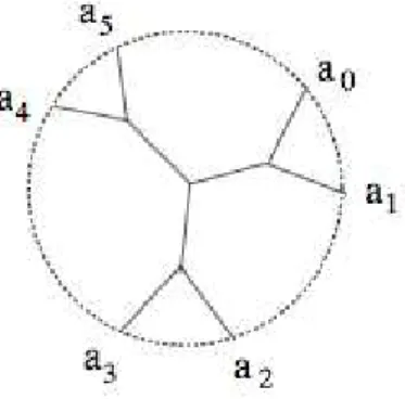
X{internal vertices of T }. Integrating such differential form, we get the integral assigned to T . If we decorate the external vertices by elements a0, . . . ,an(ai∈ S), see Figure4 . By taking the sum over

all trees T , that is decorated by a0, . . . ,an, we obtain the Hodge correlator associated to the cyclic

word W = C ({a0}⊗⋯⊗{an}) .

For the rigorous definition in details, one should refer to the work of Goncharov [10].

(16)

2.3 Examples of Hodge correlators Goncharov’s Theory of Hodge correlators

Figure 4: A plane trivalent tree decorated byC ({a0}⊗⋯⊗{a5}).

Remark 2.1 Compared to Goncharov’s setting, we will work on number field, therefore we should

find an analogue of Green’s function over number field, which is also the starting point of our construction.

2.3 Examples of Hodge correlators

Correlators on P1_C∖S and polylogarithms Let X = P1, S= {∞}. Given the following cyclic word

Wn= C ({1}⊗{z}⊗{0}⊗⋯⊗{0}),

the unique Wn-decorated Feynman diagram with no internal vertices incident to two {0}’s, see

Figure 5

Figure 5: The Feynman diagram for the classical n-logarithms.

We denote by Ln(z) the corresponding correlator [10]. Let Lin(z) be the classical n-polylogrithm

on CP1∖{0,1,∞}. Further there is a single-valued version if n oddLn(z) = Re( n−1 ∑ k=0 βklogk∣z∣⋅Lin−k(z)), if n evenLn(z) = Im( n−1 ∑ k=0 βklogk∣z∣⋅Lin−k(z)), whereβk=2 k_B k

k! , Bk is the Bernoulli number.

Then the Levin formula gives us L∗_n(z) = 4−(n−1) ∑ n∈2Z 1≤k≤n−2 (2n − k − 3 n −1 ) 2k+1 (k+1)!Ln−k(z)logk∣z∣. 14

(17)

2.3 Examples of Hodge correlators Goncharov’s Theory of Hodge correlators If we take L_n(z) = 4n−1(2n−2 n−1 ) −1 L∗_n(z).

Then Goncharov showed that the Hodge correlator can be related to the classical polylogrithms as follows

−Ln(z) = (2πi)−nLn(z).

(18)

Plectic Principle

3 Plectic Principle

3.1 Equivariant plectic Green Currents

As we have explained in the introduction, the plectic principle, we just repeat the main idea here. Let X/B be a family of abelian varities with real multiplication, and s ∶ B Ð→ X a nonzero torsion section fixed by a subgroup of finite index U⊂ O×_F,₊. This subgroup U acts naturally on X and acts trivally on B, then we should consider the following diagram

X×UEU >X

B×UEU

∨ π

>B,∨

where EU is the total space over the classifying space BU of the group U and B×UEU= B×EU/U.

When B= {pt} , then X is a variety, we have the following situation

X×UEU

BU.∨

Nekov´a˘r and Scholl [13] constructed in their work a U -equivariant current ˜θ on ˜X= X ×UR, where

UR= EU. ˜θ is a plectic generalisation of the (slightly modified) log∣θ(τ,z)∣ of the absolute value of

the standard Theta function on the elliptic curve E= C/Zτ +Z, which is the Green function on E. So s∗( ˜θ) is U-equivariant on ˜B = B×UR. Then s∗( ˜θ) can descend to a current on B×UR/U,

and we can compute the trace

π∗(s∗( ˜θ)) = ∫

UR/U

s∗( ˜θ),

which gives very interesting functions, such as generalized Eisenstein-Kronecker-Lerch series. The above integral, as well as its variants involving more complicated functions than ˜θ , can be computed by integrating suitable expressions depending on∥ux∥ over UR. For this purpose, the

Hecke transform is introduced and used in their work. Here is a typical example. In the speculative plectic conjecture[13], they consider a framework :

GL2,F⋉G2a,F < ResL/F(GL1,L)⋉G2a,F

GL2,F

∨

< Res_L_/F(GL1,L)

∨

where L is a totally imgainary quadratic extension of F. The diagram above gives rise to a Shimura stacks:

A < A_τ

Y∨< {τ} ∨

As in the previous remarks, Y is just an open Hilbert modular variety attached to GL2,F, while

A is the universal oject (in the sense of stacks) of Y. Morally A is the quotient[U/A], where A is the non-exsitent universal Hilbert-Blumenthal abelian scheme over Y (the reason is (2) of the

(19)

3.2 Some explanation of the philosophy Plectic Principle

remarks), U⊂ O×_F,₊ is a subgroup of finite index in the group of totally positive units of F. If we consider that the group U acts trivially on Y , then we can get a stack Y = [U/Y], which gives us a bigger diagram: A < A_τ Y∨ < [U/{τ}] ∨ Y∨< {τ}. ∨

3.2 Some explanation of the philosophy

In this subsection, we would like to give some geometric explanations about the reason that the subgroup U⊂ O×_F,₊plays a non-trivial role in plectic principle.

In fact a universal Hilbert-Blumenthal abelian scheme over Y doesn’t exist. First of all, we will try to explain something about the difference between two moduli problems associated to two groups. The picture is as follows:

G∗⊂ _>_G

G∨_m⊂ _>_Res

F/QGm,F

ν

∨

For an typical example, we take G= Res_F_/QGL2,F, and G∗ is defined by Cartien product (fiber

product).

G∗= {g ∈ G∣det(g) ∈ Gm}

Usually, we have the moduli problem MG∗(resp. M_G) associated to G∗(resp. G). The fact is that

the functor MG∗ is representable, which means that there is an universal abelian variety (scheme)

A_G∗over M_G∗. The group of integers of O×_F,₊acts on M_G∗,

O×_F,₊œ M_G∗, Z[F∶Q]−1≅ O×_F,+. The action of O×

F,+on the connected components is trivial. The reason is that:

Hd_{= G(R)/(K}

∞/Z(R)),

where d= [F ∶ Q] and

ZG∗(R)œ Hd/G∗(Z),

where ZG∗is the center of G∗. Therefore the center Z_G∗ acts trivially onHd/G∗(Z).

But the functor MGis just a coarse moduli space(un espace grossier in french). If we write,

Mgross

G = MG∗/O

×

F,+

(i) The neutrial component of M_Ggross= the neutrial component of MG∗.

(ii) But the set{ the connected components } of M_Ggross≠ the set { the connected components } of M_G_.

Remark 3.1 We know that the action of O×

F,+permutates the connected components of M gross G .

(20)

3.2 Some explanation of the philosophy Plectic Principle M_G∗ Mgross G p ∨ where p is a covering map (revetement).

Now we consider the previous moduli problems in the setting of stacks. Mchp

G = [MG∗/O

×

F,+]

Remark 3.2 Attention: M_Gchp is not an algebraic stack, because the group O×_F,₊ is not a finite group.

But over M_Gchp, we still have a stack :

[A /O× F,+] [Mchp G ], f ∨

where f is a representable morphism, involving a tautological abelian variety.

Now we turn to toroial compactifications. We have a diagram of compactifications for MG∗.

A_G∗ ⊂ > A_Gtor∗ O×_F,₊œ M_G∗ ∨ > M_Gtor∗ œ O×_F,₊ ∨ Similarly, there is another diagram for M_Gchp

[AG∗/O×_F,₊] > [Ator/O×_F,₊] [Mchp G ] f ∨ >[M_Gtor∗/O×_F,₊] ∨ In conclusion :

M_G∗= G∗(Q)/G∗(A)/Z_G∗(R)K_∞has a universal abelian variety.

Mgross

G = G(Q)/G(A)/ZG(R)K∞does not have a universal abelian variety.

Mchp

G = [G(Q)/G(A)/ZG(R)K∞].

(21)

Generalization of Multiple Zeta Values (I): General construction and results over Q

4 Generalization of Multiple Zeta Values (I):

General construction and results over Q

4.1 General construction

4.1.1 Plectic Green currents

In our work, we consider a generalisation of log∣1−e2πix∣2on the compact real torus

S1= {e2πix∣x ∈ R/Z} ⊂ C×.

This function is the restriction of the Green function G(1,y) = log∣1−y∣2of the origin of C×to S1. We are going to consider corresponding objects on tori with real multiplication.

Let F be a totally real field of degree r= [F ∶ Q], we have the trace map Tr = TrF/Qand the norm

map N= N_F_/Q. Let D be the different and let I be a fractional ideal of F and

I∗= {a ∈ F ∣ Tr(aI) ∈ Z} = D−1I−1.

Let∣∣ ⋅ ∣∣∶ FR= F ⊗RÐ→ R∼ Hom(F,R)Ð→ R+∪{0} be the standard euclidean norm. As above, let

UR= Ker(N ∶ (FR×)+Ð→ R×+) = {(u1, . . . ,ur) ∈ Rr+∣ u1⋯ur= 1}.

Then we can define the “plectic” Green function associated to the ideal I Definition 4.1 (Plectic Green function)

gI(x,u) = lim

η→0+ ∑ n∈I∗_/{0}

e2πiTr(nx)

∣∣un∣∣r+η , x∈ FR/I, u ∈ UR,

which can also be defined as ∑

n∈I∗_∖{0} e2πiTr(nx)

∣∣un∣∣r , viewed as a distribution on(FR/I)×UR.

We can also add an additional choice of multisignsν∈ {0,1}Hom(F,R). Then the modified ”plectic” Green function becomes

gν_I(x,u) = lim η→0+ ∑ n∈I∗_/{0} sgn(n)νe 2πiTr(nx) ∣∣un∣∣r+η ,x∈ FR/I, u ∈ UR.

There is also a second method to add a multisign

gI,ν(x,u) = lim η→0+ ∑ n∈I∗_/{0} sgn(n)=(−1)ν e2πiTr(nx) ∣∣un∣∣r+η ,x∈ FR/I, u ∈ UR. Remark 4.2 (O×_F,₊−_{equivariance)} ∀_ε∈ O× F,+, we have gI(εx,εu) = gI(x,u).

This is also true for gν_I(⋅,⋅) and gI,ν(⋅,⋅).

Remark 4.3 (Dependence on I)

1. Ifα∈ F₊×and N(α) = 1, then (αI)∗= α−1I∗. Hence gαI(αx,αu) = gI(x,u).

2. ∀α∈ F×

+, gαI(αx,u) = N(α)gI(x,u). Therefore up to rescaling, gI(⋅,⋅) depends only on the class

of I in the class group Cl_F+. This is also true for gν_I(⋅,⋅) and gI,ν(⋅,⋅).

(22)

Generalization of Multiple Zeta Values (I): General construction and results over Q 4.1.2 Higher plectic Green currents

By using just this “plectic” Green function, we will construct a function (or a distribution) GI,Γ,S(⋅,⋅)

on

O×_F,₊/(FR/I)S×UR= (FR/I)S×O×_F,₊EO×F,+,

which depends on a given graph Γ and a subset S of the set of its vertices. Definition 4.4 (Higher plectic Green function)

LetΓ be a finite connected non-oriented graph, V(Γ) the set of vertices and E(Γ) the non-empty

set of edges. Let S⊂ V(Γ) be a subset of the set of vertices. Loops are forbidden here (i.e. the endpoints of each edge are distinct), but multiple edges are allowed. For each vertex v∈ V(Γ), let xv∈ FR/I be a variable which decorates the vertex v; for each edge e ∈ E(Γ), we choose an

orientation Ð→e = (v0(e) Ð→ v1(e)) and we associate an element ne∈ I∗∖{0}.

Then the higher plectic Green function attached to(Γ,S) is

G_I,_Γ,S({x_v}_v_∈S,u) = ∫

(FR/I)V(Γ)∖S_e_∈E(Γ)∏

gI(xv1(e)−xv0(e),u) ∏

v∈V (Γ)∖S

dxv,

where xv∈ FR/I,u ∈ URand dx is a fixed Haar measure en FR, and

gI(xv1(e)−xv0(e),u) = lim η→0+ ∑

ne∈I∗/{0}

e2πiTr(ne(x_v1(e)−x_v0(e)))

∣∣une∣∣r+η

.

There are variants of these functions (and numbers) depending on an additional choice of multisigns ν(e) ∈ {0,1}Hom(F,R)_{(and an orientation) for each edge e, which means that we can replace g}

I(⋅,⋅)

by gI,ν(⋅,⋅) (or gνI(⋅,⋅)).

Remark 4.5 By the very definition, GI,Γ,S(⋅,⋅) inherits a O×F,+-invariant property. ∀ε ∈ O×F,+, we

have

G_I,_Γ,S({εx_v}_v_∈S,εu) = GI,Γ,S({xv}v∈S,u).

Therefore, our higher plectic Green function GI,Γ,S(⋅,⋅) is a function (or distribution) on

O×_F,₊/(FR/I)S×UR= (FR/I)S×O×_F,₊EO×F,+,

which depends on the given graphΓ and the subset S of the set of its vertices. Here EO×F,+is the

total space of the group O×_F,₊.

Lemma 4.6 (Convolution on FR/I) On FR/I we have a formal convolution. Let χn(x) = e2πiTr(xn).

If A(x) = ∑m∈I∗a(m)χ_m(x) and B(y) = ∑_n_∈I∗b(n)χ_n(y), then

∫_F

R/I

A(x−y)B(y)dy = ∫

FR/Im,n∑∈I∗

a(m)b(n)χm(x−y)χn(y)dy = vol(FR/I) ∑

n∈I∗

a(n)b(n)χ(n).

Proof 4.1.1 The Proof of Lemma 4.6 is straightout. ∫_F

R/I

A(x−y)B(y)dy = ∫

FR/I_m,n∑_∈I∗

a(m)b(n)e2πiTr((x−y)m)e2πiTr(yn)dy

= ∫_F

R/Im=n∑

a(m)b(n)e2πiTr(xm)e2πiTr(y(n−m))dy +_∫

FR/Im≠n∑

a(m)b(n)e2πiTr(xm)e2πiTr(y(n−m))dy.

(23)

If m≠ n, then ∫_F R/I b(n)e2πiTr(y(n−m))dy= 0. Therefore we obtain ∫_F R/I A(x−y)B(y)dy = ∫ FR/Im=n∑

a(m)b(n)e2πiTr(xm)e2πiTr(y(n−m))dy

= ∫_F R/In∈I∑∗ a(n)b(n)e2πiTr(xn)⋅∫ FR/I 1 dy= vol(FR/I) ∑ n∈I∗ a(n)b(n)e2πiTr(xn). By the definition of gI(⋅,⋅), we can rewrite the higher plectic Green function as

G_I,_Γ,S({x_v}_v∈S,u) = lim η→0+ ∑ n∶E(Γ)→I∗∖{0} ∏ e∈E(Γ) ∣∣une∣∣−r−η∫ (FR/I)V(Γ)∖S

e2πiTr(∑e∈E(Γ)ne(x_v1(e)−x_v0(e)))_d_µ

V(Γ)∖S,

(1) where we define the following map

n ∶ EÐ→ I∗_∖{0}; n ∶ e z→ n

e∈ I∗∖{0}.

Let us define the chain complex for the graph Γ.

δ ∶ C1(Γ) = Z[E(Γ)] Ð→C0(Γ) = Z[V(Γ)],

whereδ ∶(v0→ v1) z→ [v1]−[v0] is the boundary map of the chain complex and Z[X] denotes the

free abelian group on a set X. We can also define the relative chain complex for(Γ,S), namely,

C1(Γ) Ð→C0(Γ)/C0(S).

We can associate to n the following element c(n) in C1(Γ)⊗ZI∗of the graph Γ.

c(n) = ∑ e∈E(Γ) ne⋅ Ð→e ∈ C1(Γ)⊗ZI∗. If we let πv= ∑ e∈E(Γ),v1(e)=v ne− ∑ e∈E(Γ),v0(e)=v ne, (2) then

e2πiTr(∑e∈E(Γ)ne(x_v1(e)−x_v0(e)))= e2πiTr(∑v∈V (Γ)πvxv)

.

We define the boundary map

∂ n ∶ V(Γ) Ð→ I∗_,

∂ n(v) = δc(n)∣v= πv.

By using the previous convolution formula, we obtain that only the terms with∂ n∣_V_(Γ)∖S= 0 (which means that

∀_v∈ V(Γ)∖S, π_v= 0) contribute to the integral in (1). Note that

{c(n) ∣ ∂n∣V(Γ)∖S= 0} = H1(Γ,S)⊗ZI∗.

Then we get a formal Fourier convolution description of GI,Γ,S(⋅,⋅).

(24)

(25)

Generalization of Multiple Zeta Values (I): General construction and results over Q 4.1.3 Generalized MZV for totally real fields

If we suppose that there exists a subgroup U⊂ O×_F,₊of finite index stabilising{xv} for each v ∈ S, we

can apply the Hecke transform to define a new function as follows. Definition 4.11

F_I,_Γ,S({x_v}_v_∈S) = (O×_F,₊∶ U)−1_∫

UR/U

G_I,_Γ,S({x_v}_v_∈S,u)d×u, where d×u=du1⋯dur−1

u1⋯ur−1 ,∏ r

j=1uj= 1 and UR/U = BU ≅ (S)r−1is the classifying space of U ≅ Zr−1.

Remark: In the same way, we can define F_I,ν_Γ,S({xv}v∈S) and FI,ν,Γ,S({xv}v∈S).

Then the generalized multiple zeta value is defined as Definition 4.12 (Generalized Multiple Zeta Values)

Z_I(Γ,S) = F_I,_Γ,S({0}_v∈S). Remark 4.13 Similarily, we have

Z_Iν(Γ,S) = F_I,ν

Γ,S({0}v∈S),

and

Z_I,_ν(Γ,S) = F_I,_ν,Γ,S({0}_v∈S).

Remark 4.14 In fact, the construction for GI,ν,Γ(k),S({xv}v∈S,u) also works for arbitary number

fields. If a complex place exists, we can just replace the Euclidean norm by Hermitian norm and we can add signs just for the real places. For an imaginary quadratic field, there is no Hecke transform.

4.1.4 Generalized MZV for arbitary number fields

Definition 4.15 (Plectic Green functions for arbitary number fields)

Let K be a number field with r1real places(vi)1≤i≤r1 and r2complex places(wj)1≤ j≤r2and of degree

[K ∶ Q] = r1+2r2. We have the trace mapTr= TrK/Q

KR≅ Rr1×Cr2

and we have a Hermitian product

⟨ ∣ ⟩ ∶ KR×KRÐ→ C ⟨(xv,zw)∣(x′v,z′w)⟩ = ∑ v xvx′v+∑ w zwz′w, where x= (xv,zw). Let ∥⋅∥ = ⟨⋅∣⋅⟩1/2 ,

then the plectic Green function can be defined as gI(x,u) = ∑

n∈I∗_/{0}

e2πiTr(nx)

∣∣un∣∣r1+2r2, x∈ KR/I, u ∈ UR,

which is a distribution on(KR/I)×UR.

(26)

(27)

(28)

(29)

(30)

(31)

4.2 Relation to classical MZVs

= ∑ n1+n2+n3+n4=0,ni∈Z sgn(nj)=(−1)v j,1≤ j≤4 1 ∣n1∣σ1∣n2∣σ2∣n3∣σ3∣n4∣σ4 Z_I,_ν(Γ′₁,∂ Γ′₁) = ∑ n1,n2,n3∈N∖{0} 1 nσ1 1 n σ2 2 n σ3 3 (n1+n2+n3)σ4 .

Firstly, we use Eisenstein’s trick for

1 nσ2 2 n σ3 3 = ∑ r1+s1=_σ₂_+σ₃ ⎛ ⎝ Cσ2−1 r1−1 (n2+n3)r1ns1₃ + Cσ3−1 r1−1 (n2+n3)r1ns1₂ ⎞ ⎠ Then Z_I,_ν(Γ′₁,∂ Γ′₁) = ∑ r1+s1=σ₂_+σ₃ ∑ n1,n2,n3∈N∖{0} ⎛ ⎝ Cσ2−1 r1−1 (n1+n2+n3)σ4(n2+n3)r1ns1₃nσ₁1 + Cσ3−1 r1−1 (n1+n2+n3)σ4(n2+n3)r1ns1₂nσ₁1 ⎞ ⎠

Secondly, we use twice Eisenstein’s trick for the terms involving n1and(n2+n3). Then we obtain

Z_I,_ν(Γ′₁,∂ Γ′₁) = ∑ r1+s1=σ₂_+σ₃ r2+s2=r1+σ1 ∑ n1,n2,n3∈_N∖{0} C_r2r1₋₁−1Cσ2−1 r1−1 (n1+n2+n3)σ4+r2ns1₃ns2₁ + ∑ r1+s1=σ₂+σ₃ r2+s2=r1+σ1 ∑ n1,n2,n3∈N∖{0} Cσ1−1 r2−1C σ2−1 r1−1 (n1+n2+n3)σ4+r2(n2+n3)s2ns1₃ + ∑ r1+s1=σ2+σ3 r′₂+s′ 2=r1+σ1 ∑ n1,n2,n3∈_N∖{0} C_rr1′−1 2−1C σ3−1 r1−1 (n1+n2+n3)σ4+r ′ 2ns1 2n s′₂ 1 + ∑ r1+s1=σ₂_+σ₃ r′₂+s′2=r1+σ1 ∑ n1,n2,n3∈_N∖{0} Cσ1−1 r′ 2−1 Cσ3−1 r1−1 (n1+n2+n3)σ4+r ′ 2(n₂+n₃)s′2ns1 2

Finally, we use Eisenstein’s trick for the terms involving n1and n2(respectively, n1and n3).

Z_I_ν(Γ′₁,∂ Γ′₁) = ∑ r1+s1=σ2+σ3 r2+s2=r1+σ1 r3+s3=_s1_+s₂ ∑ n1,n2,n3∈_N∖{0} C_r3s1₋₁−1C_r2r1₋₁−1Cσ2−1 r1−1 (n1+n2+n3)σ4+r2(n1+n3)r3ns3₁ + ∑ r1+s1=σ₂+σ₃ r2+s2=r1+σ1 r3+s3=s1+s2 ∑ n1,n2,n3∈N∖{0} C_r3s2₋₁−1C_r2r1₋₁−1Cσ2−1 r1−1 (n1+n2+n3)σ4+r2(n1+n3)r3ns3₃ + ∑ r1+s1=σ₂+σ₃ r2+s2=_r1_+σ₁ ∑ n1,n2,n3∈N∖{0} Cσ1−1 r2−1Cσr12−1−1 (n1+n2+n3)σ4+r2(n2+n3)s2ns1₃ 29

(32)

+ ∑ r1+s1=σ2+σ3 r′₂+s′ 2=r1+σ1 r′₃+s′ 3=s1+s′2 ∑ n1,n2,n3∈N∖{0} C_rs1′−1 3−1C r1−1 r′₂−1C σ3−1 r1−1 (n1+n2+n3)σ4+r ′ 2(n₁+n₂)r′3ns ′ 3 1 + ∑ r1+s1=σ₂+σ₃ r′₂+s′ 2=r1+σ1 r′₃+s′ 3=s1+s′2 ∑ n1,n2,n3∈_N∖{0} Cs ′ 2−1 r′₃−1C r1−1 r′₂−1C σ3−1 r1−1 (n1+n2+n3)σ4+r ′ 2(n₁+n₂)r′3ns ′ 3 2 + ∑ r1+s1=σ2+σ3 r′₂+s′₂=_r1_+σ₁ ∑ n1,n2,n3∈_N∖{0} Cσ1−1 r′ 2−1 Cσ3−1 r1−1 (n1+n2+n3)σ4+r ′ 2(n₂+n₃)s′2ns1 2 Then Z_I,_ν(Γ′₁,∂ Γ′₁) = ∑ r1+s1=_σ₂_+σ₃ r2+s2=r1+σ1 r3+s3=s1+s2 (Cs1−1 r3−1C r1−1 r2−1C σ2−1 r1−1+C s2−1 r3−1C r1−1 r2−1C σ2−1 r1−1)ζ(σ4+r2,r3,s3) + ∑ r1+s1=σ2+σ3 r′₂+s′ 2=r1+σ1 r′3+s′3=s1+s′2 (Cs1−1 r′₃−1C r1−1 r₂′−1C σ3−1 r1−1 +C s′₂−1 r′₃−1C r1−1 r′₂−1C σ3−1 r1−1)ζ(σ4+r′2,r3′,s′3) + ∑ r1+s1=σ2+σ3 r2+s2=r1+σ1 Cσ1−1 r2−1C σ2−1 r1−1ζ(σ4+r2,s2,s1)+ ∑ r1+s1=σ2+σ3 r₂′+s′ 2=r1+σ1 Cσ1−1 r′₂−1C σ3−1 r1−1ζ(σ4+r2′,s′2,s1), whereσ4+r2+r3+s3= σ4+r2+s2+s1= σ1+σ2+σ3+σ4.

We can see that ZI,ν(Γ′1,∂ Γ′1) is a Z-linear combination of triple-zeta values of weight σ1+σ2+

σ3+σ4.

Example 4.25 Let Γ2be the diagram as in Figure 14.

The rank is equal to rank(H1(Γ2,∂ Γ2)) = 3. For each external edge ei(1 ≤ i ≤ 3), the given sign

νiequals0, thereforeν4= 1. G_I,_ν,Γ 2,∂ Γ2({xv}v∈S,1) = ∫ (R/Z)2 ∑ ni,mi∈Z∖{0} sgn(ni)=(−1)νi

e2πi((xv3−y)n3+(x_v4−y)n4)

∣n3∣σ3∣n4∣σ4

e2πi((xv1−z)n1+(x_v2−z)n2+(y−z)m1)

∣n1∣σ1∣n2∣σ2∣m1∣µ1

dxdy

By the formal Fourier convolution, we get

G_I,_ν,Γ 2,∂ Γ2({xv}v∈S,1) = ∑ n1+n2+m1=0,n3+n4−m1=0;ni,mi∈_Z∖{0} sgn(ni)=(−1)νi e2πi(n1xv1+n2xv2+n3xv3+n4xv4) ∣n1∣σ1∣n2∣σ2∣n3∣σ3∣n4∣σ4∣m1∣µ1 . 30

(33)

(34)

we can rewrite 1 and 2 as follows.

1 = ∑ s2+t2=σ₃+s₁+µ₁ Cσ1−1 s1−1C σ3−1 s2−1 (n1+n2+n3)s2+σ4(n1+n2)t2nt12 + ∑ s2+t2=σ₃_+s₁_+µ₁ s3+t3=t1+t2 Cσ1−1 s1−1C s1+µ1−1 s2−1 C t2−1 s3−1 (n1+n2+n3)s2+σ4(n3+n2)s3nt3₂ + ∑ s2+t2=σ3+s1+µ1 s3+t3=t1+t2 Cσ1−1 s1−1C s1+µ1−1 s2−1 C t1−1 s3−1 (n1+n2+n3)s2+σ4(n3+n2)s3nt3₃ 2 = ∑ s2+t2=σ₃+s₁+µ₁ Cσ2−1 s1−1C σ3−1 s2−1 (n1+n2+n3)s2+σ4(n1+n2)t2nt1₁ +s2+t2=∑_σ₃_+s₁_+µ₁ s′₃+t′ 3=t1+t2 Cσ2−1 s1−1C s1+µ1−1 s2−1 C t2−1 s′₃−1 (n1+n2+n3)s2+σ4(n3+n1)s ′ 3nt ′ 3 1 + ∑ s2+t2=σ3+s1+µ1 s′₃+t3′=t1+t2 Cσ2−1 s1−1C s1+µ1−1 s2−1 C t1−1 s′₃−1 (n1+n2+n3)s2+σ4(n3+n1)s ′ 3nt ′ 3 3 Finally we get: Formula 4.26 Z_I,_ν(Γ₂,∂ Γ2) = ∑ s1+t1=_σ₁_+σ₂ s2+t2=σ3+s1+µ1 ∑ n1,n2,n3∈N∖{0} Cσ1−1 s1−1C σ3−1 s2−1 (n1+n2+n3)s2+σ4(n1+n2)t2nt1₂ + ∑ s1+t1=σ₁+σ₂ s2+t2=_σ₃_+s₁_+µ₁ s3+t3=_t1_+t₂ ∑ n1,n2,n3∈_N∖{0} ⎛ ⎝ Cσ1−1 s1−1C s1+µ1−1 s2−1 C t2−1 s3−1 (n1+n2+n3)s2+σ4(n3+n2)s3nt3₂ + Cσ1−1 s1−1C s1+µ1−1 s2−1 C t1−1 s3−1 (n1+n2+n3)s2+σ4(n3+n2)s3nt3₃ ⎞ ⎠ + ∑ s1+t1=σ₁_+σ₂ s2+t2=σ3+s1+µ1 ∑ n1,n2,n3∈_N∖{0} Cσ2−1 s1−1C σ3−1 s2−1 (n1+n2+n3)s2+σ4(n1+n2)t2nt11 + ∑ s1+t1=σ₁+σ₂ s2+t2=_σ₃_+s₁_+µ₁ s′₃+t′ 3=t1+t2 ∑ n1,n2,n3∈_N∖{0} ⎛ ⎜ ⎝ Cσ2−1 s1−1C s1+µ1−1 s2−1 C t2−1 s′ 3−1 (n1+n2+n3)s2+σ4(n3+n1)s ′ 3nt ′ 3 1 + C σ2−1 s1−1C s1+µ1−1 s2−1 C t1−1 s′ 3−1 (n1+n2+n3)s2+σ4(n3+n1)s ′ 3nt ′ 3 3 ⎞ ⎟ ⎠. However, ∑ n1,n2,n3∈_N∖{0} 1 (n1+n2+n3)s2+σ4(n1+n2)t2nt1₂ = ∑0<k1<k2<k3 1 ks2+σ4 3 k t2 2k t1 1 = ζ(t1,t2,s2+σ4), where k1= n1,k2= n1+n2,k3= n1+n2+n3. Therefore Z_I,_ν(Γ₂,∂ Γ2) = ∑ s1+t1=σ₁+σ₂ s2+t2=σ3+s1+µ1 (Cσ1−1 s1−1C σ3−1 s2−1 +C σ2−1 s1−1C σ3−1 s2−1)ζ(t1,t2,s2+σ4) 32

(35)

(36)

We can use the result of 3 in the formula 4.26 to get: Z_I,_ν(Γ₃,∂ Γ3) = ∑ n1,n2,n3,n4∈N∖{0} (_∣n 1 4∣σ4∣n1+n2+n3+n4∣σ5)× ⎧⎪⎪ ⎨⎪⎪ ⎩ s1+t1∑=σ₁_+σ₂ s2+t2=σ3+s1+µ1 Cσ1−1 s1−1C σ3−1 s2−1 (n1+n2+n3)s2+µ2(n1+n2)t2nt12 ´¹¹¹¹¹¹¹¹¹¹¹¹¹¹¹¹¹¹¹¹¹¹¹¹¹¹¹¹¹¹¹¹¹¹¹¹¹¹¹¹¹¹¹¹¹¹¹¹¹¹¹¹¹¹¹¹¹¹¹¹¹¹¹¹¹¹¹¹¹¹¹¹¹¹¹¹¹¹¹¹¹¹¹¹¹¹¹¹¹¹¹¹¹¹¸¹¹¹¹¹¹¹¹¹¹¹¹¹¹¹¹¹¹¹¹¹¹¹¹¹¹¹¹¹¹¹¹¹¹¹¹¹¹¹¹¹¹¹¹¹¹¹¹¹¹¹¹¹¹¹¹¹¹¹¹¹¹¹¹¹¹¹¹¹¹¹¹¹¹¹¹¹¹¹¹¹¹¹¹¹¹¹¹¹¹¹¹¹¹¶_a + ∑ s1+t1=σ1+σ2 s2+t2=σ₃+s₁+µ₁ s3+t3=t1+t2 ⎛ ⎜⎜ ⎜⎜ ⎜⎜ ⎜ ⎝ Cσ1−1 s1−1C s1+µ1−1 s2−1 C t2−1 s3−1 (n1+n2+n3)s2+µ2(n3+n2)s3nt3₂ ´¹¹¹¹¹¹¹¹¹¹¹¹¹¹¹¹¹¹¹¹¹¹¹¹¹¹¹¹¹¹¹¹¹¹¹¹¹¹¹¹¹¹¹¹¹¹¹¹¹¹¹¹¹¹¹¹¹¹¹¹¹¹¹¹¹¹¹¹¹¹¹¹¹¹¹¹¹¹¹¹¹¹¹¹¹¹¹¹¹¹¹¹¹¹¹¸¹¹¹¹¹¹¹¹¹¹¹¹¹¹¹¹¹¹¹¹¹¹¹¹¹¹¹¹¹¹¹¹¹¹¹¹¹¹¹¹¹¹¹¹¹¹¹¹¹¹¹¹¹¹¹¹¹¹¹¹¹¹¹¹¹¹¹¹¹¹¹¹¹¹¹¹¹¹¹¹¹¹¹¹¹¹¹¹¹¹¹¹¹¹¹¶ b + C σ1−1 s1−1C s1+µ1−1 s2−1 C t1−1 s3−1 (n1+n2+n3)s2+µ2(n3+n2)s3nt3₃ ´¹¹¹¹¹¹¹¹¹¹¹¹¹¹¹¹¹¹¹¹¹¹¹¹¹¹¹¹¹¹¹¹¹¹¹¹¹¹¹¹¹¹¹¹¹¹¹¹¹¹¹¹¹¹¹¹¹¹¹¹¹¹¹¹¹¹¹¹¹¹¹¹¹¹¹¹¹¹¹¹¹¹¹¹¹¹¹¹¹¹¹¹¹¹¹¸¹¹¹¹¹¹¹¹¹¹¹¹¹¹¹¹¹¹¹¹¹¹¹¹¹¹¹¹¹¹¹¹¹¹¹¹¹¹¹¹¹¹¹¹¹¹¹¹¹¹¹¹¹¹¹¹¹¹¹¹¹¹¹¹¹¹¹¹¹¹¹¹¹¹¹¹¹¹¹¹¹¹¹¹¹¹¹¹¹¹¹¹¹¹¹¶_c ⎞ ⎟⎟ ⎟⎟ ⎟⎟ ⎟ ⎠ + ∑ s1+t1=σ1+σ2 s2+t2=σ₃+s₁+µ₁ Cσ2−1 s1−1C σ3−1 s2−1 (n1+n2+n3)s2+µ2(n1+n2)t2nt1₁ ´¹¹¹¹¹¹¹¹¹¹¹¹¹¹¹¹¹¹¹¹¹¹¹¹¹¹¹¹¹¹¹¹¹¹¹¹¹¹¹¹¹¹¹¹¹¹¹¹¹¹¹¹¹¹¹¹¹¹¹¹¹¹¹¹¹¹¹¹¹¹¹¹¹¹¹¹¹¹¹¹¹¹¹¹¹¹¹¹¹¹¹¹¹¹¸¹¹¹¹¹¹¹¹¹¹¹¹¹¹¹¹¹¹¹¹¹¹¹¹¹¹¹¹¹¹¹¹¹¹¹¹¹¹¹¹¹¹¹¹¹¹¹¹¹¹¹¹¹¹¹¹¹¹¹¹¹¹¹¹¹¹¹¹¹¹¹¹¹¹¹¹¹¹¹¹¹¹¹¹¹¹¹¹¹¹¹¹¹¹¶ d + ∑ s1+t1=σ1+σ2 s2+t2=σ₃+s₁+µ₁ s′₃+t′ 3=t1+t2 ⎛ ⎜⎜ ⎜⎜ ⎜⎜ ⎜⎜ ⎝ Cσ2−1 s1−1C s1+µ1−1 s2−1 C t2−1 s′₃−1 (n1+n2+n3)s2+µ2(n3+n1)s ′ 3nt ′ 3 1 ´¹¹¹¹¹¹¹¹¹¹¹¹¹¹¹¹¹¹¹¹¹¹¹¹¹¹¹¹¹¹¹¹¹¹¹¹¹¹¹¹¹¹¹¹¹¹¹¹¹¹¹¹¹¹¹¹¹¹¹¹¹¹¹¹¹¹¹¹¹¹¹¹¹¹¹¹¹¹¹¹¹¹¹¹¹¹¹¹¹¹¹¹¹¹¹¸¹¹¹¹¹¹¹¹¹¹¹¹¹¹¹¹¹¹¹¹¹¹¹¹¹¹¹¹¹¹¹¹¹¹¹¹¹¹¹¹¹¹¹¹¹¹¹¹¹¹¹¹¹¹¹¹¹¹¹¹¹¹¹¹¹¹¹¹¹¹¹¹¹¹¹¹¹¹¹¹¹¹¹¹¹¹¹¹¹¹¹¹¹¹¹¶_e + C σ2−1 s1−1C s1+µ1−1 s2−1 C t1−1 s′₃−1 (n1+n2+n3)s2+µ2(n3+n1)s ′ 3nt ′ 3 3 ´¹¹¹¹¹¹¹¹¹¹¹¹¹¹¹¹¹¹¹¹¹¹¹¹¹¹¹¹¹¹¹¹¹¹¹¹¹¹¹¹¹¹¹¹¹¹¹¹¹¹¹¹¹¹¹¹¹¹¹¹¹¹¹¹¹¹¹¹¹¹¹¹¹¹¹¹¹¹¹¹¹¹¹¹¹¹¹¹¹¹¹¹¹¹¹¸¹¹¹¹¹¹¹¹¹¹¹¹¹¹¹¹¹¹¹¹¹¹¹¹¹¹¹¹¹¹¹¹¹¹¹¹¹¹¹¹¹¹¹¹¹¹¹¹¹¹¹¹¹¹¹¹¹¹¹¹¹¹¹¹¹¹¹¹¹¹¹¹¹¹¹¹¹¹¹¹¹¹¹¹¹¹¹¹¹¹¹¹¹¹¹¶ f ⎞ ⎟⎟ ⎟⎟ ⎟⎟ ⎟⎟ ⎠ ⎫⎪⎪ ⎬⎪⎪ ⎭

Remark: By careful observation, we can see that on the factorisation factors (without the ex-ponent) of the denominators of these six terms a . . . f , there is an action of the symmetric group

S3. For example, to pass from the factors of the denominator of a (without considering the power)

to that of c , we letσ = σ(123) acting on (n1+ n2+ n3)(n1+ n2)n2 by (nσ⋅1+ nσ⋅2+ nσ⋅3)(nσ⋅1+

nσ⋅2)nσ⋅2, which also explains why there are6= ∣S3∣ terms.

Thanks to the remark, in order to reexpress ZI(Γ3,∂ Γ3), we only need to understand:

Sum1= ∑ n1,n2,n3,n4∈N∖{0} ( 1 nσ4 4 (n1+n2+n3+n4)σ5 )× ∑ s1+t1=σ1+σ2 s2+t2=σ₃+s₁+µ₁ Cσ1−1 s1−1C σ3−1 s2−1 (n1+n2+n3)s2+µ2(n1+n2)t2nt1₂ ´¹¹¹¹¹¹¹¹¹¹¹¹¹¹¹¹¹¹¹¹¹¹¹¹¹¹¹¹¹¹¹¹¹¹¹¹¹¹¹¹¹¹¹¹¹¹¹¹¹¹¹¹¹¹¹¹¹¹¹¹¹¹¹¹¹¹¹¹¹¹¹¹¹¹¹¹¹¹¹¹¹¹¹¹¹¹¹¹¹¹¹¹¹¹¸¹¹¹¹¹¹¹¹¹¹¹¹¹¹¹¹¹¹¹¹¹¹¹¹¹¹¹¹¹¹¹¹¹¹¹¹¹¹¹¹¹¹¹¹¹¹¹¹¹¹¹¹¹¹¹¹¹¹¹¹¹¹¹¹¹¹¹¹¹¹¹¹¹¹¹¹¹¹¹¹¹¹¹¹¹¹¹¹¹¹¹¹¹¹¶_a . (3)

Apply formula 4.23 again:

1 nσ4 4 (n1+n2+n3)s2+µ2 = ∑ s4+t4=σ₄+s₂+µ₂ ⎛ ⎝ Cσ4−1 s4−1 (n1+n2+n3+n4)s4(n1+n2+n3)t4 + Cs2+µ2−1 s4−1 (n1+n2+n3+n4)s4nt44 ⎞ ⎠. Then Sum1= ∑ n1,n2,n3,n4∈_N∖{0} ∑ s1+t1=σ₁+σ₂ s2+t2=σ3+s1+µ1 s4+t4=σ4+s2+µ2 Cσ1−1 s1−1C σ3−1 s2−1C σ4−1 s4−1 (n1+n2+n3+n4)s4+σ5(n1+n2+n3)t4(n1+n2)t2nt12 34

(37)

+ ∑ n1,n2,n3,n4∈N∖{0} ∑ s1+t1=σ1+σ2 s2+t2=σ3+s1+µ1 s4+t4=σ4+s2+µ2 Cσ1−1 s1−1C σ3−1 s2−1C s2+µ2−1 s4−1 (n1+n2+n3+n4)s4+σ5(n4)t4(n1+n2)t2nt1₂ . Again, 1 (n4)t4(n1+n2)t2 = ∑s5+t5=t4+t2 ⎛ ⎝ C_s5t4−1₋₁ (n1+n2+n4)s5(n1+n2)t5 + C_s5t2−1₋₁ (n1+n2+n4)s5nt5₄ ⎞ ⎠. Then Cσ1−1 s1−1C σ3−1 s2−1C s2+µ2−1 s4−1 (n1+n2+n3+n4)s4+σ5(n4)t4(n1+n2)t2nt1₂ = ∑s5+t5=t4+t2 Cσ1−1 s1−1C σ3−1 s2−1C s2+µ2−1 s4−1 C t4−1 s5−1 (n1+n2+n3+n4)s4+σ5(n1+n2+n4)s5(n1+n2)t5nt1₂ + C σ1−1 s1−1C σ3−1 s2−1C s2+µ2−1 s4−1 C t2−1 s5−1 (n1+n2+n3+n4)s4+σ5(n1+n2+n4)s5nt5₄nt1₂ . Once again 1 nt5₄nt1₂ = ∑s6+t6=t5+t1 ⎛ ⎝ Ct5_s6−1₋₁ (n4+n2)s6nt6₂ + C_s6t1−1₋₁ (n4+n2)s6nt6₄ ⎞ ⎠ Finally, we get Sum1= ∑ n1,n2,n3,n4∈N∖{0} ∑ s1+t1=_σ₁+σ₂ s2+t2=σ3+s1+µ1 s4+t4=σ4+s2+µ2 Cσ1−1 s1−1C σ3−1 s2−1C σ4−1 s4−1 (n1+n2+n3+n4)s4+σ5(n1+n2+n3)t4(n1+n2)t2nt1₂ + ∑ n1,n2,n3,n4∈N∖{0} ∑ s1+t1=σ₁+σ₂ s2+t2=σ3+s1+µ1 s4+t4=σ4+s2+µ2 s5+t5=t4+t2 Cσ1−1 s1−1C σ3−1 s2−1C s2+µ2−1 s4−1 C t4−1 s5−1 (n1+n2+n3+n4)s4+σ5(n1+n2+n4)s5(n1+n2)t5nt1₂ + ∑ n1,n2,n3,n4∈N∖{0} s1+t1∑=σ₁+σ₂ s2+t2=σ₃+s₁+µ₁ s4+t4=σ₄+s₂+µ₂ s5+t5=t4+t2 s6+t6=t5+t1 Cσ1−1 s1−1C σ3−1 s2−1C s2+µ2−1 s4−1 C t2−1 s5−1C t5−1 s6 (n1+n2+n3+n4)s4+σ5(n1+n2+n4)s5(n4+n2)s6nt62 + ∑ n1,n2,n3,n4∈_N∖{0} ∑ s1+t1=σ₁+σ₂ s2+t2=σ3+s1+µ1 s4+t4=σ4+s2+µ2 s5+t5=t4+t2 s6+t6=t5+t1 Cσ1−1 s1−1C σ3−1 s2−1C s2+µ2−1 s4−1 C t2−1 s5−1C t1−1 s6 (n1+n2+n3+n4)s4+σ5(n1+n2+n4)s5(n4+n2)s6nt6₄

By exchanging the sum symbols, we get

Formula 4.28 Sum1= ∑ s1+t1=σ₁+σ₂ s2+t2=σ3+s1+µ1 s4+t4=σ4+s2+µ2 Cσ1−1 s1−1C σ3−1 s2−1C σ4−1 s4−1ζ(t1,t2,t4,s4+σ5) 35