Aircraft assessment of trace compound fluxes in the atmosphere with relaxed eddy Accumulation: Sensitivity to the conditions of selection

HAL Id: hal-02354435

https://hal.archives-ouvertes.fr/hal-02354435

Submitted on 11 Jan 2021

HAL is a multi-disciplinary open access

archive for the deposit and dissemination of

sci-entific research documents, whether they are

pub-lished or not. The documents may come from

teaching and research institutions in France or

abroad, or from public or private research centers.

L’archive ouverte pluridisciplinaire HAL, est

destinée au dépôt et à la diffusion de documents

scientifiques de niveau recherche, publiés ou non,

émanant des établissements d’enseignement et de

recherche français ou étrangers, des laboratoires

publics ou privés.

Aircraft assessment of trace compound fluxes in the

atmosphere with relaxed eddy Accumulation: Sensitivity

to the conditions of selection

C. Delon, A. Druilhet, Robert Delmas, J. Greenberg

To cite this version:

C. Delon, A. Druilhet, Robert Delmas, J. Greenberg. Aircraft assessment of trace compound fluxes in

the atmosphere with relaxed eddy Accumulation: Sensitivity to the conditions of selection. Journal of

Geophysical Research: Atmospheres, American Geophysical Union, 2000, 105 (D16), pp.20461-20472.

�10.1029/2000JD900186�. �hal-02354435�

JOURNAL OF GEOPHYSICAL RESEARCH, VOL. 105, NO. D16, PAGES 20,461-20,472, AUGUST 27, 2000

Aircraft assessment

of trace compound fluxes in the

atmosphere with Relaxed Eddy Accumulation:

Sensitivity to the conditions of selection

C. Delon, A. Druilhet, and R. Delmas

Centre National de la Recherche Scientifique, UMR 5560, Laboratoire d'A•rologie, Toulouse, France

J. Greenberg

Atmospheric Chemistry Division, NCAR, Boulder, Colorado

Abstract. The Relaxed Eddy Accumulation (REA) technique, implemented aboard aircraft,

may be used to measure a wide variety of trace gas fluxes at a regional scale. Its principle is

rather simple: air is sampled at a constant rate and the flux is calculated by multiplying a

constant

[• (0.58 in field experiment

and 0.62 in simulations)

by the standard

deviation

of the

vertical velocity and by the difference between the average concentrations of the scalar (trace

gas) for updrafts and downdrafts. The storage of the chemical compound in reservoirs allows

for trace gas analysis in laboratory, when in situ measurement with fast response and high

sensitivity sensors are not available. The REA method was implemented on the Avion de

Recherche Atmosphdrique et de Tdldddtection aircraft during the Experiment for Regional

Sources and Sinks of Oxidants (EXPRESSO) campaign. The main requirement for accurate

flux determination is the measurement of the vertical component of wind velocity in real

time. A simulation technique was developed to evaluate the performance of an aircraft REA.

The influence of the time lag between the vertical velocity (W) measurement and REA

control was tested, as well as the offset of W, the threshold, and the filtering imposed on W.

Correction factors, used in a deployment of aircraft REA, were deduced from this study. An

additional simulation was performed to evaluate the influence of spatial or temporal drifts on

the scalar. The simulation showed that the REA Inethod is not more disturbed than the Eddy

Correlation method by low frequencies of physical origin, such as topography. The REA

method was used during EXPRESSO for the measurement of isoprene fluxes over the wet

savanna and the evergreen rain forest.

1. Introduction

Trace gas and energy balance between the surface and

atmosphere can be assessed by the determination of sources

and sinks at the surface and by the transfer of compounds

from the surface to atmosphere (and vice versa). Identical

constraints, concerning stationarity and homogeneity, are

applied for trace gas fluxes and energy fluxes. These fluxes

may be measured with Relaxed Eddy Accumulation (REA) and Eddy Correlation (EC) techniques, both based on atmospheric turbulence.

Constraints differ if they are applied at local (fixed point) or regional scale. For fixed points (e.g., towers) the situation is rather simple: flux measurements (like the gradient method,

the Bowen ratio method, or the Eddy Correlation (EC) method) may be made above homogeneous surfaces. In the case of aircraft flux measurements, however, since these have much larger horizontal fetch, homogeneous surfaces must be

defined statistically.

Aircraft flux techniques, including REA, are especially suited for the determination of fluxes at a regional scale and

Copyright 2000 by the American Geophysical Union. Paper number 2000JD900186.

0148-0227/00/2000JD900186509.00

from diverse ecosystems. This is particularly important •n

inaccessible regions, such as tropical forests and savannas, which usually have a strong energetic activity, high and uncharacterized species diversity, and significant importance in biogeochemical cycles.

Surface fluxes were measured from aircraft during the Experiment for Regional Sources and Sinks of Oxidants (EXPRESSO) campaign over two important ecosystems: the woodland/savanna mosaic and the evergreen rain forest. Two flux methods were employed on the Avion de Recherche

Atmosphdrique et de Tdldddtection (ARAT) aircraft: the EC

method and REA method. The EC method had already been

used to measure ozone fluxes [Lenschow et al., 1980] and has

been validated aboard the ARAT [Affre et al., 1999], with a complete methodology and a validation made using the water

vapor flux as a reference. Methods and results obtained with

the EC method during EXPRESSO are presented by Delon et al. [2000], concerning the surface energy budget and the turbulent kinetic energy budget, and were developed by B. Cros et al., (personal communication, 2000), concerning the

ozone turbulent flux measurements.

The REA method depends on the standard deviation of the vertical wind velocity Ow, the difference of the mean concentrations between updrafts and downdrafts, and an empirical constant [3. The REA method is often used to

2O,462 DELON ET AL.: RELAXED EDDY ACCUMULATION IN AIRCRAFT

measure fluxes of diverse components whose measurement with the EC method is problematic [e.g. Zhu et al., 1998] and several technical and theoretical problems have been discussed [Kramm et al., 1999]. This paper examines the calculation of the vertical velocity W in real time, an essential condition for the measurement. Alter presenting the implementation of the REA in the ARAT, we will assess several constraints which are imposed on the REA system in

the estimation of real time vertical winds. Simulations allow the evaluation of conditions of selection and of their influence

on the 13 constant and, consequently, on the evaluation of the

flux.

CO2 fluxes have been calculated with the EC method and the REA fluxes have been deduced from these calculations, in

order to evaluate the accuracy of the latter [Oncley et al., 1993]. During the EXPRESSO campaign in Central African Republic (CAR) and in the Republic of the Congo (Congo) a REA technique for isoprene fluxes [Greenberg et al., 1999] was deployed. This EC/REA comparison assesses the suitability of REA for aircraft chemical flux measurements and illustrates the influence of spatial drifts upon the scalar.

2. Presentation of the REA System Used

the Experiment

for

2.1. Theory

The Eddy Accumulation method, proposed by DesjaMins

[1972], relies on the conditional sampling of air in proportion to the vertical wind velocity (positive or negative). This method was modified by Businger and Oncley [1990] by collecting air at a constant rate for updrafts and downdrafts and was called REA. The major inconvenience of turbulent flux measurements of chemical compounds is that they require high-frequency sensors. Conditional sampling methods, like the REA, require, as with the EC method, the measurement of the turbulent component of the vertical velocity but require only average measurements of the

concentration, for which slower and selective detection

techniques exist. If the analysis cannot be performed "in situ", samples can be transported to the laboratory for analysis, which allows the measurement of vertical fluxes of a great

number of constituents [Nie et al., 1995].

The air is then collected at a constant rate, depending on the vertical velocity sign, and the vertical flux • is calculated

according to (1):

where o,•. is the standard deviation of the vertical velocity.

c+ (c-) is the mean concentration of the measured chemical

compound calculated for the sampling period in the reservoir

corresponding to the positive (negative) vertical velocity selection. Variable [3 is a constant, approximately 0.58 in field experiments [Pattey et al., 1993] and 0.62 in simulations [Businger and Oncley, 1990; Wyngaard and Moeng, 1992]. Simulations show that 13 is weakly dependent on the stability [Businger and Oncley, 1990; Andreas et al., 1998].

2.2. Implementation in the ARAT Aircraft for the

EXPRESSO Campaign

The REA method has been widely used on ground [e.g.,

Baker et al., 1992; Guenther et al., 1996b; Bowling et al., 1998]. It requires, among other conditions, a homogeneous

emission source and high-frequency measurement of vertical velocity, usually with sonic anemometers. REA ground measurements have been performed for several chemical compound fluxes, for example, isoprene (nonmethane hydrocarbons) (Guenther et al., 1999; Zhu et al., 1999] or

ozone [Katul et al., 1996].

An REA was installed in the French ARAT research

aircraft for the EXPRESSO campaign, which took place in

CAR from November 15 to December 2, 1996 (an overview

of the experiment is given by Delmas et al., [1999]).

EXPRESSO was an interdisciplinary experiment, whose

purpose was to study exchange processes between biosphere and atmosphere in tropical regions, and to quantify the impact of emissions on atmospheric chemical composition at a regional scale. Three different experimental platforms were

used in EXPRESSO: a 60-m-high walk-up tower situated in

the undisturbed primary forest of the northern Congo,

dedicated to local-scale measurements (N'Doki, 2ø12N, 16ø23E); the ARAT instrumented aircraft, for regional-scale measurements, and two stations receiving signals at a continental scale from the National Oceanic and Atmospheric Administration - Advanced Very High Resolution Radiometer (NOAA-AVHRR) satellite. There were 11 research flights, 4 above wet savanna vegetation and 5 above evergreen rain

forest vegetation. Two additional flights were made over the

forest/savanna interface. The flights were carried out daily

between 0930 and 1230 local time. The installation of the

REA in the ARAT is detailed in Figure 1.

2.3. Cycle of the REA Measurement

A cycle of measurement was composed of the following

sequence: (1) 4 min for sampling of eddies into up- and down-draft reservoirs along a constant attitude and altitude

leg; (2) 1 min for transfer of aliquot of air from the reservoirs onto adsorbent cartridges, for later analysis of isoprene; (3) 30

s (+30 s) for analyzing the positive selection (+ negative

selection) for CO2; and (4) 2 min, 30 s for evacuating the

reservoirs and reinitializing the cycle.

For iw

I greater

than the threshold

the sampled

air was

forwarded (through two Teflon tubes) to two Teflon reservoirs, situated at the back of the plane (corresponding to point 1 in the detail of the cycle above). Air from each reservoir was sampled onto solid adsorbent cartridges for later

analysis of isoprene (point 2). Reservoir air was analyzed for CO2 using a Licor LI-6262 CO2/H20 Analyzer (point 3).

When the Licor analyzer was not taking air from the reservoirs, it took air from outside (point 4). This allowed the measurement of the mean CO2 concentration during the whole

flight, except during the minute of analysis when the analyzer took air from the reservoirs. The cycle and the position of the

system in the ARAT are schematized in Figure 1.

3. Real Time Vertical Velocity Measurement

One of the most important technical problems of the REA

method in the aircraft is the real-time determination of

vertical velocity W. The first attempts made by MacPherson and Desjardins [1991] were not conclusive. Thus in the ARAT aircraft the first objective was to calculate an instantaneous W, since W, computed by the standard aircraft data system, contributed an unacceptable delay of

approximately 0.25 s, due to the transfer rate of the numerical message (Figure 2).

DELON ET AL.' RELAXED EDDY ACCUMULATION IN AIRCRAFT 20,463

REA

computer

depending on the W sign. from analog and numerical data.

W<threshold (expulsion) W>0 REA SYSTEM IN THE ARAT W <0

Control

computer

of

the REA cycle (automat) selection/analyze/emptying

Storage of

ii'.:• :•::::•:.,: ii.:':•i '::.,..•:.:..: and neg afiv e sel ecfi o ns switching control R+

CO2/H20

Reference

gas

J

II

•[ Chamber2

[•

Exterior

air )

I

( •ii

il

!ii

iii!i•

[

•[

Chamber

Bags emptying I I

'1

Figure 1. Scheme

of the REA system

aboard

the ARAT. Open

circles

correspond

to the three-way

switching

valves,

and gray

ellipses

correspond

to inlet (-•) or outlet

(•-) pumps.

The two reservoirs

are represented

by

open

rectangles.

R+ (R-), reservoir

corresponding

to the selection

of positive

(negative)

vertical

velocity.

3.1. Calculation of the Simplified WRF•^

The Inertial Navigation System (INS) aboard the ARAT provides position, velocity, and acceleration data. These data are transmitted in a numerical form to a computer called Systbme de Fabrication d'Instruments de Mesure, SFIM,

Figure 2). SFIM receives analog signals coming from the

different sensors (detailed by Delmas et al. [1999]), transforms them into numerical signals, and classfries and transmits to the data acquisition system of the aircraft. This

acquisition system calculates a vertical velocity of air with

high resolution, but the data are stored and transmitted every

quarter second, too long a delay for the REA control in real time. A separate computer was thus inserted to calculate a

simplified vertical velocity, WREA. This "REA computer" takes information concerning the pitching (0) and the vertical velocity of the aircraft (Wa) from the INS and transfers air speed and incidence from the SFIM to compute WREA,

according to the expression

W, .... = (i - O)u + Wa +113 (2)

where l 0 is the vertical velocity induced by rotation, l (16 m) is the distance between the boom extremity and the gravity center;

Wa is the aircraft vertical velocity related to the ground; Wa=(dz./dt) where z is the coupled baroinertial height (Wa is

given by the INS); (i - O)u is the air velocity related to the

aircraft. During stable flight, i = 0 (attack angle = pitch angle). If the aircraft is influenced by gales, i differs from 0. Almost all information concerning the turbulence is contained in this term.

• ,

Variable •,=v•,+v•, , where • is the average air speed of the

aircraft (ranging from 80 to 100 m/s) and v,, is the horizontal velocity fluctuation (around 1 m/s).

The calculated WREA has to be converted from numerical to analog data needed by the REA control computer. This analog signal is then transmitted to the WR•A computer through a band-

pass filter (between 0.02 and 10 Hz). A 10-Hz (0.1 s) low-pass

filter is necessary to remove the noise induced by the calculation and the conversion from analog to numerical data (and vice versa), and to limit the electrovans (solenoid valve) switching tYequency. A 0.02 Hz (50 s) high-pass filter is essential to reject low-frequency components (whose scale is greater than 5 km) and to eliminate the offsets induced by the calculation (see below).

The REA control computer is programmed to execute and control the cycle of measurement and operation of the electrovans for the wind selection. The air selection, depending

20,464 DELON ET AL.' RELAXED EDDY ACCUMULATION IN AIRCRAFT

INS

Analogical

data Information every 1/64 s

REA computer

V•ea = ( i--• ) U+Wa +l •

transfer rate 1/4 s

SFIM

computer

Bata.

d-pass

Acquisition on board Central computer Control computer of thc REA (automat)

Figure 2. Scheme of the calculation of the simplified REA velocity (WRE^) from the reference velocity (WREF) calculated by the central computer on board.

on the vertical velocity direction, is made above a threshold equivalent to 0.10w (where cs• is the standard deviation of W). If the threshold is greater than 0.1o}•., the deadband effect is too large to ensure an accurate flux measurement (deadband is a range of vertical wind velocity when no sample is collected). In

the interval of +0. lOw, the sign of the vertical velocity is

ambiguous, and the selection of air is not representative of the

flux direction. Variable Ow can be either specified •br each leg,

depending on the preceding measurement, or fixed between 0.6 and 1 rn/s (values usually encountered in the convective boundary layer [Caughey and Palmer, 1979]). This simplified and filtered velocity W}•^ is re-injected into the SFIM in order to be compared to the reference velocity WRE F. The comparison

gives a good correlation on low-level legs (Figure 3) and

allowing W}•EA tO be used without systematic error for the air

selection.

3.2. Simulated Functions

The REA method is called a "blind" method because of the

impossibility of controlling the conditions of selection (i.e., vertical wind velocity over 0.1 c•). Several technical problems may occur, depending on these conditions of selection (switching frequency, delays, etc.). Computational time may also interfere and influence the delay in the calculation of the vertical velocity, the band-pass filtering, or the threshold used for the selection of the vertical velocity. The calculation of

y = 0.9495x + 0.2463

R

2 = 0.944

2

Figure 3. WRE A (REA vertical velocity) and WRE F (reference vertical velocity) in m/s during a 5-min low-

level leg (310 m) of flight 45 (savanna flight performed during the EXPRESSO campaign on November 24,

1996). The equation

corresponds

to the regression

between

W•E^

and W•EF,

and R 2 is the correlation

DELON ET AL.' RELAXED EDDY ACCUMULATION IN AIRCRAFT 20,465 Arbitrary Units (a) 10 -3 Arbitrary (b) Units W X Spectrum peak '- [ , ' ", ... i ... i'-""/"-'•-'i'"-i--

I Frequency

ban• 1

[ • •.•::ii:

i:;

•

ii:.i

•

•:

•/ arøund

spectrum

the

peak

i I I i i I J J J J J I J J J J ] I I J I J

10 2 I(Y • 1 10 •

Frequency (Hertz)

0 2 3 4

Time (min.)

Figure 4. (a) Simulation of functions from an energy spectrum: x axis, frequency in Hz; y axis, arbitrary units. The gray rectangle gives the position of the frequency band around the spectrum peak. (b) W (vertical velocity) and X (scalar) are shown as examples of functions: x axis, time; y axis, arbitrary units.

fluxes of chemical compounds with the REA method assumes

that w =0. But in real conditions of selection, tiffs is not

always the case. Computations, made from simulated

variables, were used to assess the influence of different problems encountered in real conditions, such as the difference from zero of the average vertical velocity (offset), the threshold imposed on the vertical velocity sampling, the time lag between reference vertical velocity calculated by the

aircraft (WREF) and simplified vertical velocity calculated for- the REA command (WRE^), and the filtering of REA vertical

velocity.

The quality of the REA measurement is modeled from a

collection of simulated variables, where homogeneity and

stability are controlled statistically. In each simulation, the

product Ow(C+-C-) is compared to the covariance directly

calculated with the EC method, which allows the determination of the •3 constant and an evaluation of its

dependence on each parameter (offset, threshold, or time lag).

Four variables

are represented

for each

simulation:

(1) the •3

constant, (2) the concentration in the reservoir corresponding

to updrafts (C+) minus the mean concentration, and (3) the

concentration in the reservoir corresponding to downdrafts

(C-) minus the mean concentration, both normalized by the

standard deviation of the concentration, and (4) the flux

(J3ow(C+-C-)) normalized by a reference flux (I)0. This

reference flux is constant and does not vary when [•, C+ and

C- change. All these variables are nondimensional

(normalized) and therefore represented on the same y axis

(see Figures 5, 6, and 7).

The simulation method used here relies on random time series with known statistical properties. The turbulent functions correspond to the ones found in the boundary layer. W and X (vertical velocity and scalar, respectively) are built from a theoretical spectrum shape (Figure 4a). The turbulence

scale corresponds to the nS(n) maximum (where n is the

aircraft frequency). S(n) has a-5/3 slope in the inertial

subrange,

and nS(n) has a +l slope in the low-frequency

range. The correlation between W and X is defined by the

frequency band around the spectrum peak (Figure 4a). The

bandwidth allows the determination of the value of the correlation coefficient between W and X. An example of times series of W and X is shown in Figure 4b.

A sensitivity study for two different conditions of turbulence was conducted to describe the influence of

constraints imposed on flux measurement. The first case corresponds to a flight performed for the evaluation of surface

fluxes (Z = 50 m, aircraft speed = 90 m/s), and the second

case corresponds to the evaluation of entrainment fluxes, near

the top of the boundary

layer (Z = 1200 m, aircraft

speed

=

100 m/s).

Zi = 1500

m is the thickness

of the boundary

layer.

The REA characteristics

depend

on the wavelength

of the

spectrum peak of the vertical velocity. Near the surface (50

m) this wavelength 3, is about 5 times the altitude where the

aircraft flies (3, = 5xZ = 5x50 m = 250 m) and then tends

toward

1.5Zi when

the aircraft

flies at the top of the boundary

layer (X, = 1.5x1500 m = 2250 m) [Caughey

and Palmer,

1979; Druilhet et at., 1983]. The contribution of coherent

20,466 DELON ET AL.' RELAXED EDDY ACCUMULATION IN AIRCRAFT 'o o I.•.2 _. o G+ 0.4- 0 [ ] [ [ -1 -0.8 -0.6 -0.4 -0.2 0 0.2 0.4 0.6 0.8 1 Offset ((7 •) 'o o 1.4- _. •/•o

oc+

Figure 5. Sensitivity of the REA variables to the vertical velocity offset for two flight levels: (a) 50 m (0.03Zi) and (b) 1200 m (0.8Zi). The offset is given proportionally to {5,• (standard deviation of the vertical velocity). The REA variables are the [3 constant, C+/oc, C-/oc, and •/•o. Variable Oc is the standard

deviation of the concentration.

about 3 to 6 times the thickness of the boundary layer [Lohou et al., 1998], far above the actual aircraft sampling altitudes.

3.2.1. Sensitivity to the vertical velocity offset. Approximations of aircraft vertical velocity and attack angle

are needed in the calculation of W in real time. The aircraft

vertical velocity is calculated from INS data, which depends on the baroinertial coupling and may produce an offset of the order of 10 cm/s. W is difficult to control in practice, since the attack angle is difficult to define accurately. However, if the calibration is made off-line, the average components can be removed by a filtering or by stating the condition that w =o.

Figure 5 illustrates the influence of the offset on the REA variables 13, C+/oc, C-/oo and •/•0 near the surface (0.03Zi)

on Figure 5a and near the top of the boundary layer (0.8Zi) on Figure 5b. The offset of W is given proportionally to Ow. The

result depends strongly on the statistical characteristics and the nonstationarity of the variables. For surface fluxes the variables are stationary and close to Gaussian variables. When

the offset is negative (positive), the positive (negative)

fraction increases. Consequently, the slightest skewness on

the vertical velocity will produce a discontinuity on the result, through the effect on C+ and C-, related to the dependence of 13 on Ow.(Figure 5a).

The nonstationarity of 13 (and •/•0) increases with the

spectral scale. In Figure 5b, as the offset decreases, 13 and •/•0 increase, while C+ and C- decrease. In figure 5b (where

DELON ET AL.: RELAXED EDDY ACCUMULATION IN AIRCRAFT 20,467 a 1.2 1 =0.8 ,-- =0.6 O.2 0 0.05 0.1 0.15 0.2 0.25 0.3 0.35 0.4 0.45 Threshold ((•w) 0.5 1.2 1 0 0.05 m 0.8 E o ,-- 0.6 m 0.4 > et- 0.2 o o o _. o c+ -A-C- 0.1 0.15 0.2 0.25 0.3 0.35 0.4 0.45 0.5 Threshold ((•w)

Figure 6. Sensitivity

of the REA variables

(same

as in Figure

5) to the threshold

(a) at 50 m (0.03Zi) and (b)

at 1200 xn (0.8Zi). The threshold is given proportionally to o•,.

Z=1200 m) the spectral scale is greater than that near the surface (Figure 5a), and [3 and (I)/(I) 0 increase rapidly when the

offset is negative. To avoid these effects, the average vertical velocity must be kept equal to zero. On the ARAT, a band- pass filtering was imposed on the W}•E^ in order to meet this

condition.

3.2.2. Sensitivity to the vertical velocity threshold. In

order to limit the electrovan switching frequency and avoid sampling around weak vertical velocities (so as to increase the concentration difference subsequently measured in the

reservoirs), a threshold is fixed on the vertical velocity

selection and air is not sampled into up or down reservoirs

when the vertical winds are less than the threshold

(deadband). Figure 6 illustrates the influence of the threshold

on the REA variables (the threshold is proportional to o,•,, and ranges from 0 to 0.5o,•,), near the ground (Figure 6a), and at

0.8Zi, (Figure 6b). A similar result was reported by Pattey et al. [1993] and Katul et al. [1996] for ground fluxes

measurements: [3 decreases as the threshold increases. When

the threshold increases the REA variables are influenced the

same way near the ground and near the top of the boundary layer. In both cases the flux decrease is about 10% for a threshold equivalent to 0.1 o,•.. The difference in

concentrations measured in the reservoirs increases

significantly with the threshold. Consequently, the sensitivity of the measurement will be improved in the limit of 0.1o,,. Beyond this limit the diminution of the REA variables does

not involve a realistic value of the flux anymore.

3.2.3. Sensitivity to the vertical velocity selection delay (time lag). The dependence of the REA variables with the time lag is illustrated on Figure 7 (0.03Zi on Figure 7a and 0.8Zi on Figure 7b). Near the surface the REA variables,

20,468 DELON ET AL.' RELAXED EDDY ACCUMULATION IN AIRCRAFT a 5 4

'• 2

Time lag (seconds)

o

0 0.2 0.4 0.6 0.8 1 1.2

Time lag (seconds)

Figure 7. Sensitivity of the REA variables (same as in Figure 5) to the vertical velocity delay (time lag, in

seconds) (a) at 50 m (0.03Zi) and (b) at 1200 m (0.8Zi).

especially ]3 and •/•o, are strongly dependent on the increase

of the time lag. Indeed, when Z = 50 m, the time needed to run the spectral scale (X, = 250 m) is T = 250/90 = 2.8 s, which

is not negligible against the time lag (e.g. 0.2 s). As the delay increases, a point of discontinuity is involved (Figure 7a). On the contrary, at the top of the boundary layer, the increase of

the delay has practically no influence. When Z=1200 m

(X, = 2250 m), T = 2250/100 = 22.5 s is far greater than the

time lag: the point of discontinuity is not reached. The

influence of this point of discontinuity on the flux is very bad and leads to an unrealistic result. The importance of obtaining

the smallest delay between WRE^ and WREF is emphasized.

Consequently,

the delay did not exceed

0.1 s during

the

EXPRESSO campaign.

3.2.4. Sensitivity

to the low-pass

filtering. Low-pass

filtering

is essential

to the calculation

of vertical

velocity

in

real time: it smoothes

the digital noise,

applied

by the REA

computer, and it limits the switching frequency. A high-pass

filtering

ensures

that the mean

vertical

velocity

W is equal

to

zero. Near the surface the REA variables are very sensitive to

the low-pass filtering, whose effect is the same as the one of

the increasing time lag. At the top of the boundary layer the

influence

of the low-pass

filtering

is rather

weak

(the filtering

has also the same influence as the time lag). Precise real time vertical velocity measurements are, consequently, required to restrict the effect of the low-pass filtering on REA control.

4. Influence of Space-Dependent

Drifts

The REA may be affected

by several

technical

problems

referenced

above

but may also

be influenced

by the physical

characteristics of the scalar. In order to illustrate the influence

of a nonstationary scalar, we used CO2 fluxes data measured

by EC and

REA techniques

during

the EXPRESSO

campaign.

The calculation of CO2 fluxes with the REA method and with

DELON ET AL.: RELAXED EDDY ACCUMULATION IN AIRCRAFT 20,469 (a) C02 concentration (ppm) 367/ 360 346 0 10 20 Distance (km) (b) Altitude (m) 4OO 2OO 0 ) 0 10 20 Distance (km)

Figure 8. Spatial drift of the CO2 concentration on three low-level legs of flight 47 (forest flight performed

during the EXPRESSO campaign on November 26 1996). (a) CO: concentration (in ppm) is plotted

according to the distance covered by the aircraft. (b) The three CO: plots correspond to the three legs of the aircraft, whose altitude is represented. The fourth plot corresponds to the averaged ground level during the legs.

Altitude

of

the

legs

/'

of the CO 2 concentration recorded during the flights. This simulation allows the evaluation of the influence of spatial drifts (which may be associated with physical low frequencies), encountered on the scalar. This evaluation is made by comparison between the directly measured CO2 concentration and this same signal after a high-pass filtering.

Most of the spatial drifts are the result of the aircraft motion. Figure 8 illustrates the evolution of CO2 concentration (Figure 8a) on three low-level legs performed during flight 47 (forest flight, top part of Figure 8b). The fourth line in the bottom part of Figure 8b shows the ground level topography. The legs are performed at three different altitudes, above the same ground path and using contrary directions. The 10 ppm decrease (or increase, depending on the direction of the leg) in the CO2 concentration recurs from one leg to the other (on a 20-km horizontal path). REA CO2 simulated fluxes are compared to CO2 fluxes computed with

the EC method in order to evaluate the influence of spatial

drifts. A delayed filtering is applied on REA fluxes to remove the low-frequency CO2 fluctuations. The calculation of a turbulent flux (with the EC method) is made in two different ways: the raw calculation uses all the spectral characteristics

of the scalar and the filtered calculation eliminates all the

wavelengths greater than 3Zi.

These functions were also used for the comparison of CO2 fluxes with the REA method. Raw and filtered fluxes of both

methods are compared on Figures 9a and 9b for 15 aircraft

legs performed in the boundary layer at different altitudes. The REA constant 13 is 0.58 in the calculation (this value is

usually used with physical functions).

Regressions values are good: 0.96 and 0.72 for filtered and raw fluxes, respectively. Although the regression value is

weaker for raw fluxes, the correlation between the two fluxes

remains favorable. This highlights an important and new

result: it is well known that the EC method is weakly affected

by low frequencies

on the scalar;

this comparison

shows

that

the REA method is not more affected by spatial drifts than the EC method. Fluxes calculated with the experimental REA

(and not simulated) are raw, and, consequently, low

frequencies do not increase the uncertainty of the fluxes. The raw flux/filtered flux ratio evaluated with the EC

method for another scalar presenting the same kind of low

frequencies as /'or the CO2 can be easily calculated. An

estimation of filtered REA fluxes can then be calculated, by

applying it to raw REA fluxes. This ratio, calculated during

the EXPRESSO campaign for water vapor, is close to 1 near

the surface and reaches 1.5 at the top of the boundary layer,

where the role of low frequencies induced by entrainment

processes is enhanced.

5. Isoprene Flux Measurements During

EXPRESSO Campaign

the

The isoprene measurement was performed by a team from the National Center for Atmospheric Research, Atmospheric Chemistry Division [Greenberg et aI., 1999]. Isoprene was trapped onto solid adsorbent cartridges and then analyzed in the laboratory after the experiment. The cartridges were a three-stage combination (from weakest to strongest adsorbent) of glass beads, Carbotrap©, and Carbosieve S-III© [Greenberg et aI., 1999]. Cartridges were stored at approximately-30øC before and after flights, except during transport to and from the CAR. During transport, the cartridges were kept in an ice chest (0øC-5øC); transport time was approximately 30 hours. Samples were analyzed by gas chromatography with flame ionization and atomic emission detectors for quantitation and mass spectrometry for peak identifications. Details of analytical procedures and techniques are given by Greenberg et aI. [1994].

Isoprene fluxes are plotted on Figure 10 for each type of ecosystem. This ecosystem classification was made from the analysis of AVHRR satellite data. The areas where REA

20,470 DELON ET AL.: RELAXED EDDY ACCUMULATION IN AIRCRAFT 1600 1400 - 1200 -

lOOO

-

FOREST

I

I Bø*;i

Figure 9. (a) REA raw fluxes

compared

to EC raw fluxes.

(b) REA filtered

fluxes

compared

to EC filtered

fluxes.

All the

fluxes

are

in ppb.m.s

-•. The

equations

correspond

to the

regression

line

(solid

black

line).

R 2 is

the correlation coefficient.

(a) 600 '• 500

• 400

R

2

=

0.7246 •

Eddy Correlation CO2fluxes(ppb.m.ff •)

6OO

(b) 300

R

2

= 0.9683

& •

Eddy Correlation CO2 fluxes (ppb.m.s '•)

Figure

10. Isoprene

flux measurements

made

above

the

forest

and

the savanna,

according

to the latitude.

As

the

vegetation

varies

with

latitude,

the

x axis

could

have

also

been

related

to the

vegetation.

Two

points

only

are available

for each

ecosystem,

but each

point

is an average

of several

measurements.

Consequently,

vertical

bars correspond

to error bars,

and horizontal

bars

correspond

to the extension

in latitude

of the

DELON ET AL.: RELAXED EDDY ACCUMULATION IN AIRCRAFT 20,471

isoprene fluxes were made were of two types. The savanna near Boali (coordinates: 4øN, 18øE) was very similar to the surrounding savanna over which REA measurements were made, so these measurements were included as one average

value for savanna isoprene flux. The same was true for the

tropical forest: the landscape surrounding Enyfilfi

(coordinates: 2øN, 17øE) was indistinguishable from other

forest landscapes where we made REA measurements. So an average forest isoprene flux was also calculated. The savanna is actually classified as degraded woodland, which means that it was formerly tropical forest but has been subjected to

repeated burns. The satellite vegetation database shows that

the area where REA measurements were made corresponded to one land use classification (degraded woodland). The forest REA area was a mosaic of two land use categories: seasonal tropical forest and primary rainforest. The forest and degraded woodland landscapes can also be reclassified into approximately 20 sublandscapes each, but these mostly contain varying amounts of the same species. This may explain some of the variability of emissions measured over the landscapes, especially the forest area.

Isoprene fluxes over the Enydl6 forest are about 980

gg/m:/h

(0.27 gg/m:/s),

while they are about

900 gg/m2/h

(0.25 gg/m:/s)

over

all forests

flown

over

during

EXPRESSO.

(These quantities are similar because of the similarity of the

studied ecosystems.) Isoprene fluxes over the savanna are

about

550 gg/m:/h

(0.15 gg/m2/s).

Isoprene fluxes were also measured on the N'Doki tower a few meters above the canopy. Mean midday fluxes (1000 LT

and 1400

LT) were about

1400 [tg/m:/h

in March

and 460

gg/m:/h in November (D. Serga et al., personal

communication, 2000). These above-canopy and aircraft

measurements were compared to the results of model

evaluations [Guenther et al., 1999]. The results of the model

prediction were in good agreement (within a factor of 2) with experimental data, but field measurements are needed to

parameterize the model for tropical landscapes.

6. Conclusion

The REA system deployed on the ARAT aircraft for the EXPRESSO campaign allowed the measurement of isoprene

fluxes over the savanna and the forest. The REA method

allows the direct measurement of vertical eddy fluxes, where

fast-response physicochemical analyzers for EC measurements are unavailable. The accuracy of REA depends most critically on the accurate determination of vertical velocity of air in real time. A parallel and independent calculation vertical velocity algorithm (WREA) was developed for the EXPRESSO campaign, and offline comparisons

between the two vertical velocities, WREA and WREF show a

very good agreement. Constraints, linked to the introduction of filtering imposed to obtain w =0 were evaluated in order

to define their influence on the measurement accuracy. Two conditions of turbulence, at the surface (0.03Zi) and in the entrainment zone (0.8Zi), were simulated. Four points were developed:

1.The offset on WREA, the vertical velocity which controls

the REA, may introduce an error in the resulting flux, which is corrected, in part, by a band-pass filter. This error may

reach 15% at 0.8 Zi for an offset of 0.2 •. (Table 1 and Figure 5).

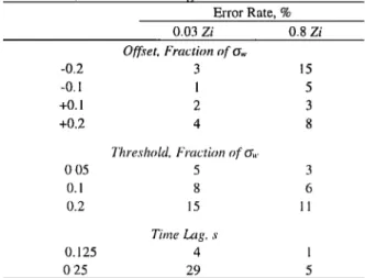
Table 1. Error Rate of tl•e Flux When the Offset, the

Threshold, and the Time Lag Increase

Error Rate, % 0.03 Zi 0.8 Zi Offset, Fraction qf cr• -0.2 3 15 -0.1 1 5 +0.1 2 3 +0.2 4 8

Threshold, Fraction qf cy,

0.05 5 3 0.1 8 6 0.2 15 11 Time Lag, s 0.125 4 1 0.25 29 5

Variable o,• is the standard deviation of the vertical velocity.

2.The introduction of a threshold on the REA vertical

velocity helps to enhance the method sensitivity (Table 1 and

Figure 6).

3.For the entrainment flux the time lag (between vetical

velocity measurement and REA selection) does not have a big

influence up to 1 s, but this delay must not exceed 0.1 s for the surface flux (the error rate increases up to 29% when the delay exceeds 0.125 s (Table 1 and Figure 7)).

4.The low-pass filtering effect is similar to the time lag: the

filtering does not have a big influence at 0.8Zi, but the influence is very important near the surface.

The only way to avoid these effects is to ensure a WR•A the

closest to WR•F. These simulations, made a posteriori, may

eventually improve the calculation of WREA, made in real time. The correction factors can be deduced directly from the error

rates reported in Table 1. Additional simulations made with CO: concentrations show that the REA method is not more

affected by low frequencies (spatial or temporal drifts of the

scalar) than the EC method. The determination of a filtered flux/raw flux ratio of water vapor by EC, for instance, allows the evaluation of REA off-line filtered fluxes. The solving of technical problems encountered when the vertical velocity is

measured is an additional step to ensure the accuracy and the

reliability of REA flux measurements. Results obtained by

REA isoprene fluxes are similar to isoprene REA tower fluxes made during the same period and area of the EXPRESSO

campaign.

References

Affre, C., A. Carrata, F. Lefebre, A. Druilhet, J. Fontan, and A. Lopez, Aircraft measurement of ozone turbulent flux in the atmospheric boundary layer, Atmos. Environ., 33, 1561-1574,

1999.

Andreas, E.L., R.J. Hill, J.R. Gosz, D.I. Moore, W.D. Otto, and A.D. Sarma, Stability dependence of the eddy accumulation coefficients for momentum and scalars, Boundary Layer

Meteorol., 86, 409-420, 1998.

Baker, J.M., J.M. Norman, and W.L. Bland, Field scale application of flux measurement by conditional sampling, Agric. For. Meteorol.,

62:31-52, 1992.

Bowling, D.R., A.A. Turnipseed, A.C. Delany, D.D. Baldocchi, J.P. Greenberg, and R.K. Monson, The use of Relaxed Eddy Accumulation to measure biosphere-atmosphere exchange of

20,472 DELON ET AL.: RELAXED EDDY ACCUMULATION IN AIRCRAFT

isoprene and other biological trace gases, Oecologia, 116: 306-

315, 1998.

Businger, J.A., and S.P. Oncley, Flux measurement with conditional sampling, J. Atmos. Oceanic Technol. 7, 349-352, 1990.

Caughey, S.J., and S.G. Palmer, Some aspects of turbulence structure through the depth of the convective boundary layer, Q. J. R.

Meteorol. Soc., 105, 811-827, 1979.

Delmas, R., et al., Experiment for Regional Sources and Sinks of

Oxidants (EXPRESSO): An overview, J. Geophys. Res.,

104(D23), 30,609-30,624, 1999.

Delon, C., A. Druilhet, R. Delmas, and P. Durand, Dynamic and thermodynamic structure of the lower troposphere above rain forest and wet savanna during the EXPRESSO campaign, J. Geophys. Res., 105, 14,823-14840, 2000.

Desjardins, R.L., A study of carbon dioxide and sensible heat fluxes using the eddy correlation technique. Ph.D. dissertation, 189 pp.,

Cornell Univ., Ithaca, N.Y., 1972.

Druilhet, A., J.P. Frangi, D. Guedalia, and J. Fontan, Experimental studies of the turbulence structure parameters of the convective boundary layer, J. Clim. Appl. Meteorol., 22 (4), 594-608, 1983. Greenberg, J.P., B. Lee, D. Hehning, and P.R. Zimmerman, Fully

automated gas chromatograph-flame ionization detector system for the in situ determination of atmospheric non-methane hydrocarbons a• low parts per trillion concentration, J. Chromatogr. A, 676, 389-398, 1994.

Greenberg, J.P., A. Guenther, S. Mandronich, W. Baugh, P. Ginoux, A. Druilhet, R. Delmas, and C. Delon, Biogenic VOC emissions

in central Africa during the EXPRESSO biomass burning season,

J. Geophys. Res., 104, 30,659-30,671, 1999.

Guenther, A.P., P. Zimmerman, L. Klinger, J. Greenberg, C. Ennis, K. Davis, W. Pollock, H. Westberg, G. Allwine, and C. Geron, Estimates of regional natural volatile organic compound fluxes from enclosure and ambient measurements, J. Geophys. Res., 101,

1345-1359, 1996a.

Guenther, A., et al., Isoprene fluxes measured by enclosure, relaxed eddy accumulation, surface layer gradient, mixed layer gradient, and mixed layel' mass balance techniques, J. Geophys. Res., 101,

18,555-18,567, 1996b.

Guenther, A., W. Baugh, G. Brasseur, J. Greenberg, P. Harley, L. Klinger, D. Ser9a, and L. Viefling, Isoprene emission estimates and uncertainties for the Central African EXPRESSO study domain, J. Geophys. Res., 104, 30,625-30,639, 1999.

Katul, G.G., P.L. Finkelstein, J.F. Clarke, and T.G. Ellestad, An investigation of the conditional sampling method used to estimate fluxes of active, reactive and passive scalers, J. Appl. Meteorol.,

35, 1835-1845, 1996.

Kramm, G., N. Beier, R. Dlugi, and H. Mtiller, Evaluation of conditional sampling methods, Contrib. Atmos. Phys., 72, 161-

172, 1999.

Lenshow, D.H., A.C. Delany, B.B. Stankov, and D.H. Stedman,

Airborne measurements of the vertical flux of ozone in the

boundary layer, Boundary Layer Meteorol., 19, 249-265, 1980. Lohou, F., B. Campistron, A. Druilhet, P. Foster, and J.P. Pages,

Turbulence and coherent organizations in the Atmospheric Boundary Layer: A RADAR-Aircraft experimental approach, Boundary Layer Meteorol. 96, 147-179, 1998.

MacPherson, J.I., and R. Desjardins, Airborne tests of flux measurement by relaxed eddy accumulation technique, paper presented at 7 "• Symposium on Meteorological Observations and Instrumentations, Am. Meteorol. Soc., Boston, Mass., 14-18 January, 1991.

Nie, D., J.E. Kleindienst, R.R. Arnst, and J.E. Sickles, The design and testing of a Relaxed Eddy Accumulation system, J. Geophys.

Res., 100, 11,415-11,423, 1995.

Oncley, S.P., A.C. Delany, T.W. Horst, and P.P. Tans, Verification of flux measurement using Relaxed Eddy Accumulation, Atmos.

Environ., 27A, 2417-2426, 1993.

Pattey, E., R.L., Desjardins, and P. Rochetie, Accuracy of the Relaxed Eddy Accumulation technique, evaluated using CO2 flux measurements, Boundary Layer Meteorol., 66, 341-355, 1993. Wyngaard, J.C., and C.H. Moeng, Parameterizing turbulent diffusion

through the joint probability density, Boundary Layer Meteorol,

60, 1-13, 1992.

Zhu, T., R.L. Desjardins, J.I MacPherson, E. Pattey, and G. St.

Amour, Aircraft measurements of the concentration and flux of

agrochemicals, Environ. Sci. Technol., 32, 1032-1038, 1998. Zhu, T., D. Wang, R.L. Desjardins, and J.I. MacPherson, Aircraft-

based volatile organic compounds flux measurements with relaxed eddy accumulation, Atmos. Environ., 33, 1969-1979, 1999.

R. Delmas, C. Delon, and A. Druilhet, UMR Centre National de la Recherche Scientifique/Universitd Paul Sabatier 5560, Laboratoire d'Adrologie, 14 avenue Edouard Belin, 31400 Toulouse, France. (delc @ aero.obs-mip.fr)

J.P. Greenberg, National Center for Atmospheric Research, Atmospheric Chemistry Division, P.O. Box 3000, Boulder, Colorado

80307-3000.

(Received November 23, 1999; revised March 6, 2000; accepted March 10, 2000.)