Physical controls on orographic cirrus inhomogeneity

HAL Id: hal-00296292

https://hal.archives-ouvertes.fr/hal-00296292

Submitted on 23 Jul 2007

HAL is a multi-disciplinary open access

archive for the deposit and dissemination of

sci-entific research documents, whether they are

pub-lished or not. The documents may come from

teaching and research institutions in France or

abroad, or from public or private research centers.

L’archive ouverte pluridisciplinaire HAL, est

destinée au dépôt et à la diffusion de documents

scientifiques de niveau recherche, publiés ou non,

émanant des établissements d’enseignement et de

recherche français ou étrangers, des laboratoires

publics ou privés.

J. E. Kay, Mark D. Baker, D. Hegg

To cite this version:

J. E. Kay, Mark D. Baker, D. Hegg. Physical controls on orographic cirrus inhomogeneity.

At-mospheric Chemistry and Physics, European Geosciences Union, 2007, 7 (14), pp.3771-3781.

�hal-00296292�

www.atmos-chem-phys.net/7/3771/2007/ © Author(s) 2007. This work is licensed under a Creative Commons License.

Chemistry

and Physics

Physical controls on orographic cirrus inhomogeneity

J. E. Kay1, M. Baker2, and D. Hegg2

1_{National Center for Atmospheric Research, Boulder, CO, USA}

2_{Department of Atmospheric Sciences, University of Washington, Seattle, WA, USA}

Received: 5 March 2007 – Published in Atmos. Chem. Phys. Discuss.: 10 April 2007 Revised: 17 July 2007 – Accepted: 17 July 2007 – Published: 23 July 2007

Abstract. Optical depth distributions (P(σ )) are a useful

measure of radiatively important cirrus (Ci) inhomogene-ity. Yet, the relationship between P(σ ) and underlying cloud physical processes remains unclear. In this study, we investi-gate the influence of homogeneous and heterogeneous freez-ing processes, ice particle growth and fallout, and mesoscale vertical velocity fluctuations on P(σ ) shape during an oro-graphic Ci event. We evaluate Lagrangian Ci evolution along kinematic trajectories from a mesoscale weather model (MM5) using an adiabatic parcel model with binned ice mi-crophysics. Although the presence of ice nuclei increased model cloud cover, our results highlight the importance of homogeneous freezing and mesoscale vertical velocity vari-ability in controlling Ci P(σ ) shape along realistic upper tro-pospheric trajectories.

1 Introduction

1.1 Background

Cirrus clouds (Ci), layer clouds that are entirely glaciated, are often optically inhomogeneous. Neglecting Ci optical depth (σ ) inhomogeneity can lead to large biases in computed ra-diative fluxes (Fu et al., 2000; Carlin et al., 2002). One useful measure of Ci inhomogeneity is an optical depth distribution P(σ ), i.e., the fraction of σ occurring at a given σ . Under-standing physical controls on Ci P(σ ) should improve repre-sentation of radiative fluxes in weather and climate models.

In general, Ci σ can be approximated as:

σ = 2π Reff2Nice1Z (1)

where Reffis the ice crystal effective radius [m], Niceis num-ber concentration of ice crystals [m−3_{], and 1Z is the Ci} cloud layer thickness [m].

Correspondence to: J. E. Kay ([email protected])

From Eq. (1), we find that for a fixed ice Reffand 1Z, Ci

σ are determined primarily by Nice. At a fixed ice water

con-tent (temperature), Reffis largely determined by Nice. There-fore, understanding physical controls on Ci Niceis a first-step towards understanding physical controls on Ci P(σ ).

K¨archer and Str¨om (2003) and Hoyle et al. (2005) con-cluded that homogeneous freezing and small scale variability (frequencies (ν [h−1_{]) up to 10 h}−1_{or spatial scales <11 km)} in vertical velocity (w [m s−1_{])) controlled Nicedistributions} measured during the INCA and SUCCESS field campaigns. Haag and K¨archer (2004) found that background number concentrations of ice nuclei (NI N) reduced modeled Nice, but that IN presence did not significantly alter overall Ci prop-erties and formation locations. Kay (2006) noted that ob-served NI N (NI N<0.1 cm−3 (DeMott et al., 2003; Rogers et al., 1998)) and homogeneous freezing at weak synoptic-scale w (w≪5 cm s−1 _{(Mace et al., 2001)) could not} ex-plain the mean observed Niceat Lamont, Oklahoma (USA)

(Nice=0.1 cm−3, Mace et al., 2001). Taken together, these

studies suggest that observed Ci Nicecan be largely explained by homogeneous freezing occurring at a range of w. These studies also imply that heterogeneous freezing alone cannot explain observed Ci Nice.

Kay et al. (2006) (hereafter K06) assessed physical con-trols on Lagrangian P(σ ) along constant lifting trajectories. For a typical range of w, temperatures (T [K]), and NI N, σ and P(σ ) shape depended primarily on w. The sensitiv-ity of σ to w resulted for two reasons: 1) As w increased, Ci Niceincreased, Reffdecreased, and the initial σ increased (see Eq. 1). 2) As Reffdecreased, fallout timescales (τfallout [s]) and cloud lifetimes increased. In other words, the w dur-ing freezdur-ing controlled both the initial σ and the σ evolution. In contrast, the addition of IN to lifting parcels had a limited influence on modeled σ . The addition of observed NI Nonly reduced σ and modified P(σ ) with large w. With small w, IN had little influence on the calculated σ and P(σ ) because IN quickly fell out of the parcel, and because the Nicegenerated

Time (UTC) 0 24 20 16 12 8 4 H ei gh t (k m ) 6 15 12 9 D ep ol ar iza tio n (% ) 0 50 30 20 40 10 A. 190 220 210 230 200 240 255 250 260 245 10 .7 µ m B rig htn es s Te m pe ra tu re (K ) ^ ^ ^ ^ ^ ^ ^ ^ ^ ^ ^ ^ ^ ^ ^ ^ ^ ^

*

*

*

*

*

*

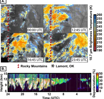
Fig. 1. Infrared satellite and lidar depolarization observations on

19 April 2001: (A) GOES infrared satellite image time series. Low brightness temperatures indicate high cloud tops. (B) Vertically pointing lidar depolarization ratio observations from Lamont. High depolarization ratios (>10%) indicate ice.

by homogeneous freezing at low w were comparable to ob-served NI N.

Given the importance of w to Ci Niceand P(σ ), the influ-ence of realistic w sequinflu-ences on Ci formation and evolution should be evaluated. Unfortunately, it is difficult to predict air flow and measure w along Ci evolution pathways. With the exception of wave cloud studies (e.g., INTACC (Field et al., 2001), FIRE II (Heymsfield and Miloshevich, 1995)), there is a dearth of Lagrangian w observations. As a sub-stitute for measuring Lagrangian w in the atmosphere, pre-vious studies (e.g., Hoyle et al., 2005; Haag and K¨archer, 2004) have statistically constructed Lagrangian w trajecto-ries. In these studies, observed distributions of small-scale w were superimposed on Lagrangian displacement trajectories derived from large-scale atmospheric models (horizontal res-olution >40 km). Because Lagrangian w measurements are difficult to obtain, and because statistically constructed w tra-jectories are not necessarily realistic, kinematic tratra-jectories extracted from mesoscale weather models (4 km < horizon-tal resolution < 40 km) could serve as a useful proxy for La-grangian w observations. Mesoscale weather model trajecto-ries capture mesoscale w variability (2 h−1_{<ν<10 h}−1_{) and} provide a realistic and self-consistent measure of Lagrangian w evolution.

1.2 Study goals and organization

In this study, we investigate physical controls on oro-graphic Ci P(σ ) using the K06 parcel model and w tra-jectories derived from the PSU/NCAR mesoscale model (MM5) (Grell et al., 1994). We selected an orographic Ci case study because mountainous terrain provides a natu-ral laboratory for investigating the influence of mesoscale

(2 h−1_{<ν<10 h}−1_{) w variability (w=1–300 cm s}−1_{, cooling}

rates =1–100 K h−1_{) on Ci P(σ ), and because orographic Ci} are often missed by climate models (Dean et al., 2005). We note that orographic Ci typically form in environments with larger w than non-orographic Ci.

In Sect. 2, we introduce the orographic Ci case study using observations. In Sect. 3, we present and evaluate the mete-orology and w forecasted by MM5. In Sect. 4, we describe both our methods for estimating σ evolution with the K06 parcel model and our trajectory parcel model experiments. Section 5 contains our results: we evaluate the influence of w and IN on Ci P(σ ) calculated along realistic upper tro-pospheric trajectories. We compare parcel model Ci to the Ci generated by a standard MM5 bulk microphysics scheme, the Reisner II scheme (Reisner et al., 1998). Their inter-comparison is interesting because the Reisner II scheme ne-glects the influence of w on Ci Nice. In fact, the Nice pre-dicted by the Reisner II scheme at Ci formation temperatures (T <−30◦_{C) is a constant Nice=0.1 cm}−3_{. Finally, we assess} which physical factors could explain the observed Ci forma-tion and broad P(σ ). Secforma-tion 6 contains a summary and dis-cussion of our results.

2 19 April 2001 Ci observations

On 19 April 2001, orographic Ci formation and evolution was observed by the GOES infrared satellite and a vertically pointing Raman lidar located at Lamont, Oklahoma (OK), hereafter Lamont (Fig. 1). From 06:00 to 16:00 UTC, oro-graphic Ci formed in the lee of the Southern Rocky Moun-tains. The Ci were then advected East with the upper level winds. Approximately 5 to 6 h after formation, the Ci were observed by the lidar above Lamont.

The lidar-observed Ci had a constant cloud top height of approximately 12.7 km, but a cloud base that varied from 6.5 to 11 km (Fig. 1). Two independent σ retrievals, one based on emissivity shape in the atmospheric window retrieved from Atmospheric Emitted Radiance Interferometer (AERI) ob-servations (Turner, 2005), and the other based on Beer’s law and the lidar backscatter below and above cloud, were gener-ally consistent when σ <3. Retrieved Ci σ increased mono-tonically from 06:00 to 12:00 UTC and then varied from σ <0.1 to σ ∼3 (Fig. 2). From 12:00 to 24:00 UTC, σ vari-ability resulted in a broad P(σ ) (Fig. 2). The lidar observa-tions reveal that 1Z variaobserva-tions contributed to the observed broad P(σ ) (Fig. 2). Although the lidar observations do not

0.0 0.1 0.2 0.3 Optical Depth (σ) Li da r P(σ ) 0 1 2 3 12-24 UTC 0-12 UTC B. Time (UTC) 0 4 8 12 16 20 24 AERI Lidar O pti ca l D ep th (σ ) 0 3 5 4 2 1 A. O pti ca l D ep th (σ ) 0 3 2 1 Cloud Thickness (∆Z, km) 0 1 2 3 4 5 6 C.

Fig. 2. 19 April 2001 σ observations: (A) σ time series. Time

series of Ci σ based on two independent retrieval methods (AERI, lidar). (B) 12-h lidar-derived P(σ ). (C) lidar-derived σ vs. physical cloud thickness from 08:00 to 24:00 UTC.

reveal the influence of Niceand Reff on the observed σ , the large amount of scatter in the observed relationship between σ and 1Z shows that the observed 1Z variability explains only a small fraction of the observed σ variability (Fig. 2).

3 19 April 2001 MM5 forecast

3.1 MM5 methods

We ran the MM5 with three nested domains for the 19 April 2001 orographic Ci event both to forecast the meteo-rology, and to enable calculation of Lagrangian w trajecto-ries (Fig. 3, Table 1). All MM5 domains included the Front Range of the Rocky Mountains, where the Ci formed, and Lamont, where the Ci passed overhead (Fig. 1).

3.2 MM5 meteorology

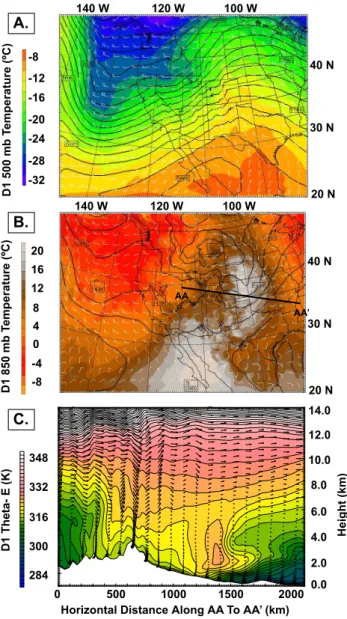
At 12:00 UTC on 19 April 2001, the MM5 forecasted a broad upper-level ridge over the central United States, a low pres-sure system developing in Montana, and a trough in the lee of the Rocky Mountains (Fig. 4). Both the developing Montana low and the lee trough contributed to a weak North-South trending warm front. A cross section of equivalent potential temperatures shows the lee trough, a cold front aloft above

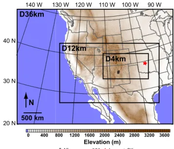
140 W 130 W 120 W 110 W 100 W 90 W 20 N 30 N 40 N N ฀15 115 0 400 800 1200 1600 2000 2400 2800 3200 3600 Elevation (m) D36km D12km D4km 500 km # #Albuquerque,฀NM Lamont,฀OK

Fig. 3. MM5 domain configuration used for the 19 April 2001

forecast.

Table 1. MM5 V3.7.3 configuration.

MM5 model specification Value Forecast duration 36 h

Forecast start 12:00 UTC 18 April 2001 Domain spatial resolution 36 km, 12 km, 4 km Domain temporal resolution 240 s, 80 s, 27 s Vertical extent 50 levels, 0 to 100 km Vertical resolution 500 m from 6 to 13 km Initialization NCEP/NCAR Reanalysis Microphysics parameterization Reisner II Cumulus parameterization Kain Fritsch Shallow convection option None Radiation parameterization CCM2

Nudging None

the Rockies, and a warm front approaching Northern OK (Fig. 4). Circulation vectors with the mean motion of the cold front removed demonstrate that air above 8 km had net westerly air flow.

Although the MM5 forecast (Fig. 4) was broadly consis-tent with the National Weather Service (NWS) reanalysis at 850 mb and 500 mb, the MM5 had a stronger and tighter Montana low, and a reduced gradient in, and lower overall, 500 mb geopotential heights over the Rockies. In the South Central USA, these model geopotential height biases indi-cate that the MM5 forecast had lower wind speeds over the Rockies, and weaker frontal lifting than what was observed.

20 N 30 N 40 N 100 W 120 W 140 W D 1 50 0 m b Te m pe ra tu re (º C ) -8 -12 -16 -20 -24 -32 -28 D 1 85 0 m b Te m pe ra tu re (º C ) 20 16 12 8 4 0 -8 -4 14.0 2.0 4.0 6.0 8.0 10.0 12.0 0.0 20 N 30 N 40 N 100 W 120 W 140 W H ei gh t (k m ) 0 500 1000 1500 2000

Horizontal Distance Along AA To AA’ (km)

AA AA’ A. B. C. D 1 Th eta - E (K ) 348 332 316 300 284

Fig. 4. MM5 meteorology at 12:00 UTC on 19 April 2001 (A)

500 mb temperatures and geopotential heights (B) 850 mb tempera-tures and geopotential heights. (C) Cross section through AA-AA′_.

Circulation vectors have the mean speed of the cold front removed (12.7 m s−1_).

3.3 MM5 vertical velocities

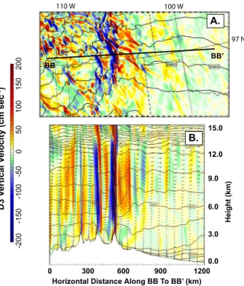
Above the Southern Rockies in central New Mexico and Col-orado, MM5 forecasted vertically propagating orographic gravity waves with large (w>100 cm s−1_{) and variable w} (Fig. 5). The strongest vertical motions resulted from 12:00 to 15:00 UTC when the upper level winds were perpendic-ular to the Rockies and the cold front aloft approached the Western edge of the lee trough. Downwind of the Rockies,

w were generally small (w<30 cm s−1_).

Using the MM5 wind fields, we calculated Lagrangian w trajectories associated with the observed Ci formation and evolution (Table 2). Our calculations indicate that air from

Table 2. Lagrangian MM5 trajectories.

Trajectory parameter Value MM5 domain D36km, D4km

Duration 8 h

Temporal resolution 3.6 min End time above Lamont 08:00 to 24:00 UTC End height above Lamont 12 km Total number 266

Eastern New Mexico and Colorado traveled over the South-ern Rockies, and arrived above Lamont in approximately 8 h. The MM5 domain resolution influenced the amplitude and spatial scale of w variability along the trajectories (Fig. 6). Trajectories derived from the MM5 domain with 4-km spa-tial resolution (D4km) had a larger range of w than trajecto-ries derived from the MM5 domain with 36-km spatial res-olution (D36km). The D4km trajectories also had greater spectral power at mesoscale frequencies (spatial equivalent 20–60 km) than the D36km trajectories. Neither set of tra-jectories had small-scale variability in w because neither do-main resolved dynamics occurring at small scales (ν>6 h−1_, spatial equivalent <18 km).

The sensitivity of the modeled w to MM5 domain resolu-tion and the lack of w observaresolu-tions made it difficult to quan-titatively validate the MM5-forecasted w. As a result, we qualitatively assessed the MM5 w forecasts within the con-text of the two main drivers of orographic wave development: the mountain range topography and the upwind atmospheric stability and wind profile (Durran, 2003).

Mountain wave theory suggests that given the large width of the Front Range, vertically propagating hydrostatic waves should result for most atmospheric stability and wind pro-files (Durran, 2003). The D4km w are consistent with this theory (Fig. 5). With the relatively steep leeward slope of the Front Range, idealized calculations suggest hydrostatic grav-ity waves could generate positive displacement at Ci heights (see Fig. 20.11 in Durran, 2003). At upper levels, MM5 fore-casted persistent positive w at heights of 6–12 km in the lee of the Rockies (Fig. 5).

To evaluate the representation of the upstream wind and stability profiles, we compared the modeled and observed soundings at Albuquerque, New Mexico (ABQ) (Figs. 7, 3). The MM5 ABQ sounding was qualitatively similar to the observed ABQ sounding. Both soundings had a stable at-mospheric potential temperature profile and increasing wind speed with height. Differences between the MM5 and the ob-served ABQ sounding included: 1) the MM5 sounding was more stable and 2) the MM5 ABQ sounding had less vertical wind speed shear above 8 km. Despite these differences, the MM5 representation of wind and stability profiles provided confidence in the forecasted gravity wave development.

20 0 15 0 10 0 50 0 -2 00 -5 0 -1 50 -1 00 D 3 Ve rti ca l V el oc ity (c m s ec -1) 110฀W 100฀W BB BB’ A. 97฀N 15.0 3.0 6.0 9.0 12.0 0.0 H ei gh t (k m ) 0 300 600 900 1200

Horizontal Distance Along BB To BB’ (km)

B.

Fig. 5. MM5 vertical velocities at 12:00 UTC on 19 April 2001. (A) D4km 300 mb w (B) D4km w cross section. Location of cross

section BB-BB′_{is indicated on (A).}

4 Parcel model methods

4.1 Conceptual framework

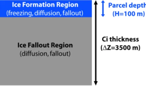
In this study, we evaluate Ci processes occurring along La-grangian w trajectories using the K06 parcel model and a simple conceptual framework (Fig. 8).

The K06 model includes heterogeneous and homogeneous freezing, vapor diffusion, and fallout. Fallout is calculated by assuming that a fraction of the ice particles fall out of the parcel in each time step. This fallout fraction is determined individually for each bin using the particle fall speed, the timestep, and the assumed parcel depth (H [m]).

The key assumption in our conceptual framework is that processes occurring in an ice formation region near cloud top control P(σ ) shape. We model freezing, vapor diffusion, and fallout occurring in this ice formation region with the K06 parcel model. We then calculate Ci σ evolution using Eq. (1) by linearly scaling the ice formation region Reffand Niceover the entire cloud depth and by assuming 1z=3500 m (the mean observed 1Z from 08:00 to 24:00 UTC, see Fig. 2). Finally, we calculate Ci P(σ ) and other distributions such as P(Nice) over the duration of the modeled Lagrangian evolu-tion.

Within our conceptual framework, it is easy to understand and to quantify interactions between complex dynamics and Ci microphysical processes. In an adiabatic parcel model

fol-0.00 0.05 0.10 0.15 0.20 0.25

Vertical velocity (w) (cm sec-1₎

P(w ) A. 0 2 4 6 8 10 12 14 16 18 20 D36km Frequency (hr-1₎ Spatial equivalent (km) B. D 3 6 k m Sp e c tr a l Po w e r (x 1 0 fo r D 4 k m ) D4km 99% limits red noise 0 Inf 1.8 60 3.6 30 5.4 20 7.2 15 9.0 12 10.8 10 -300 -200 -100 0 100 200 300 D36km D4km

Fig. 6. The effect of MM5 domain resolution on vertical velocity

amplitude and frequency structure along Ci Lagrangian evolution pathways. A horizontal wind speed of 30 m s−1_{was assumed in all}

spatial equivalence calculations.

0 2 4 6 8 10 12 14 16 270 290 310 330 350 370 390 MM5 D4km observed H ei gh t (k m ) Potential Temperature (K) 0 10 20 30 40 50 MM5 D4km observed Wind Speed (m/s) A. B.

Fig. 7. ABQ 04/19/2001 12 UTC sounding comparison: (A) MM5

D4km vs. observed stability profile (B) MM5 D4km vs. observed wind speed profile.

lowing a Lagrangian displacement trajectory, the time and location of a new freezing event (i.e., when dNice

dt increases

above a specified threshold) is controlled both by the ini-tial conditions, which set the total displacement required to start freezing, and by the displacement trajectory. If homo-geneous freezing begins, the maximum supersaturation with respect to ice largely controls the maximum homogeneous nucleation rate (Jhom−max[m−3s−1]) and the resulting Nice. If heterogeneous freezing begins, NI N and the IN freezing threshold determine the resulting Nice. Once Ci form, their σ evolution and P (σ ) shape are determined by the shortest

Table 3. Description of parcel model (PM) exper-iments: All PM experiments are named as follows: PM MM5Domain INparameterization(if applicable). All parcels were initialized with sulfuric acid aerosols (dry mass =10−16_kg,

Naer=100 cm−3). Parcel initial conditions (T, RHice, P) and w

tra-jectories were derived from the indicated MM5 domain. All parcels were assumed to be adiabatic, which implies that no mixing or nudging to the MM5 fields was included. All background IN froze at a shifted water activity equivalent to freezing at RH_ice=130% (see K¨archer and Lohmann, 2003).

Experiment name MM5 domain IN PM D4km D4km none PM D4km IN D4km Background IN PM D4km Meyers D4km Meyers et al. (1992) PM D36km D36km none

microphysical and dynamical timescales (see K06). Because the parcel model is a zero-dimensional model, the computa-tional requirements for estimating interactions between real-istic dynamics derived from a three-dimensional numerical weather model and binned microphysics are minimal.

Despite the described advantages, there are limitations as-sociated with our methodology for estimating Ci σ evolu-tion (see also K06 and Kay, 2006). For simplicity, we use a constant depth of the ice formation region (the parcel depth H ) and a constant 1z. Neither of these assumptions is com-pletely realistic. First, 100 m is a reasonable, but ad hoc, esti-mate for H . Cloud evolution in the K06 model is sensitive to H and vertically resolved cloud processes would be more re-alistic. Fortunately, K06 found that σ trends and P(σ ) shapes are largely independent of reasonable H values. Second, us-ing a constant scalus-ing of the formation region properties to obtain an integrated Ci σ cannot always be justified. For ex-ample, observations show that 1Z variability contributes to σ variability (Fig. 2). Because we assume a constant 1Z, we can only incorporate σ variability associated with variability in w and initial conditions such as NI N. A more complex model could be used to predict 1Z and to assess the contri-bution of 1Z variability to σ variability. The fidelity of 1Z predictions derived from a more complex model will largely depend on the assumed vertical moisture profile.

4.2 Parcel model runs

Guided by the observed Ci cloud top and timing (Fig. 1), we focused our Ci modeling efforts on trajectories ending 12 km above Lamont (Table 2). We calculated Ci evolution using the K06 adiabatic parcel model with variable initial condi-tions and w trajectories (Table 3). By comparing P(σ ) calcu-lated along w trajectories derived from the D36km and D4km MM5 domains, we evaluated the influence of mesoscale w variability and w amplitude on Ci formation and evolution.

Ice฀Formation฀Region (freezing,฀diffusion,฀fallout) Ice฀Fallout฀Region (diffusion,฀fallout) Parcel฀depth ฀(H=100฀m) Ci฀thickness (∆Z=3500฀m)

Fig. 8. Ci conceptual framework.

We also evaluated the effect of IN on Ci P(σ ) by initializing parcels with either a fixed background concentration based on observations (NI N=0.03 cm−3) or the NI Npredicted by Meyers et al. (1992), a commonly-used model IN parame-terization in which the NI Nincreases exponentially with the vapor supersaturation with respect to ice.

5 Results

5.1 Overview of results

The Lagrangian dynamical forcing along the MM5 w trajec-tories revealed large-scale cooling and mesoscale variability in w in the lee of the Rockies. Both the kinematic forcing and the initial conditions affected Ci processes modeled along the Lagrangian trajectories. Our parcel model results demon-strate that mesoscale w variability associated with orographic gravity waves broadened Ci P(σ ) shape. In contrast, the addi-tion of typical background NI N(NI N=0.03 cm−3) to parcels had a limited influence on modeled Ci σ variability, but did increase overall modeled Ci cloud cover. Finally, the inho-mogeneity, but not the timing, of the observed Ci was repro-duced by our Ci parcel modeling along MM5 trajectories.

5.2 Lagrangian forcing

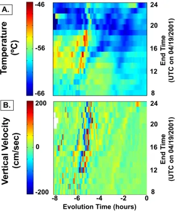
Lagrangian T and w time-time plots from the D4km MM5 domain show the forcing important for Ci formation and evo-lution on 19 April 2001 (Fig. 9). All air parcels traveled over the high topography of the Southern Rocky Mountains be-tween evolution times –7 and –5 h, i.e., 5 to 7 h before arrival at Lamont. In the lee of the Rocky Mountains, air parcels experienced cooling, and variable w associated with the ver-tically propagating orographic gravity waves (Fig. 5). For the last 4 h prior to arrival at Lamont, air parcels had small vertical motions (w<30 cm s−1_{). Widespread cooling} oc-curred between evolution times –3 and –2 h, while warming occurred along trajectories in the two hours prior to arrival above Lamont.

Te

m

pe

ra

tu

re

(º

C

)

Ve

rti

ca

l V

el

oc

ity

(c

m

/s

ec

)

8 24 En d Ti m e (U TC o n 04 /1 9/ 20 01 ) 12 16 20 8 24 En d Ti m e (U TC o n 04 /1 9/ 20 01 ) 12 16 20 -46 -66 -56 A. B.

Fig. 9. Temperature and vertical velocity along Lagrangian

trajec-tories derived from the D4km MM5 domain: These time-time plots show the Lagrangian evolution of the MM5 kinematic forcing on air parcels arriving 12 km above Lamont. The y-axis indicates the parcel arrival time at Lamont. The x-axis indicates the evolution time, i.e., the time before parcel arrival at Lamont.

5.3 Parcel model Ci

Consistent with observations (Fig. 1), cooling in the lee of the Rockies resulted in parcel model Ci formation from 06:00 to 16:00 UTC, i.e., between evolution times –6 and –4 h for trajectories arriving above Lamont from 12:00 to 20:00 UTC (Fig. 10). Variability in the large-scale cooling, the mesoscale w amplitude and timing, and the initial con-ditions resulted in a range of parcel modeled Ci formation times, Nice, σ , and cloud lifetimes along the Lagrangian tra-jectories. From the parcel model Ci results, three general Ci formation and evolution sequences could be categorized by arrival time at Lamont:

1. Along trajectories arriving from 12:00 to 14:00 UTC, Ci formed by homogeneous freezing at evolution time –5 h, but Ci then sublimated in descending motions. Af-ter a cloud-free period, a second homogeneous freezing event occurred at evolution time –3 h and these Ci per-sisted to Lamont.

2. Along trajectories arriving from 15:00 to 20:00 UTC, Ci formed from evolution time –5 to –3 h. Variability in w led to a range of Niceand cloud lifetimes. Only the

tra-Nice (# c m -3) σ 9 0 3 -8 -6 -4 -2 0 Evolution Time (hours)

8 24 En d Ti m e (U TC o n 04 /1 9/ 20 01 ) 12 16 20 8 24 En d Ti m e (U TC o n 04 /1 9/ 20 01 ) 12 16 20 5 0 2.5 A. B. PM_D4km Nice -8 -6 -4 -2 0 Evolution Time (hours)

PM_D4km_IN Nice

PM_D4km σ

C.

D. PM_D4km_IN σ

-8 -6 -4 -2 0

Evolution Time (hours) -8Evolution Time (hours)-6 -4 -2 0

6

Fig. 10. Parcel model Ci along hourly trajectories: Nice and σ

from the parcel model are plotted along Lagrangian trajectories end-ing every hour 12 km above Lamont. White indicates no cloud was present (IWC <0.01 mg m−3_{). See Table 3 for parcel model}

config-uration details and naming conventions. See Fig. 9 for a description of time-time plots.

jectories with large Niceand limited descending motion persisted over many hours and arrived at Lamont.

3. Along trajectories arriving from 21:00 to 24:00 UTC, Ci formed from evolution time –8 to –7 h, but few Ci formed in the lee of the Rockies, and no Ci arrived at Lamont.

The addition of background IN to air parcels resulted in changes to the timing and magnitude of homogeneous freez-ing along individual trajectories; however, the overall loca-tion of cloud formaloca-tion in the lee of the Rockies, the variabil-ity in Niceand cloud lifetimes, and the quantity of Ci arriving at Lamont were not altered by the addition of background IN (Fig. 10).

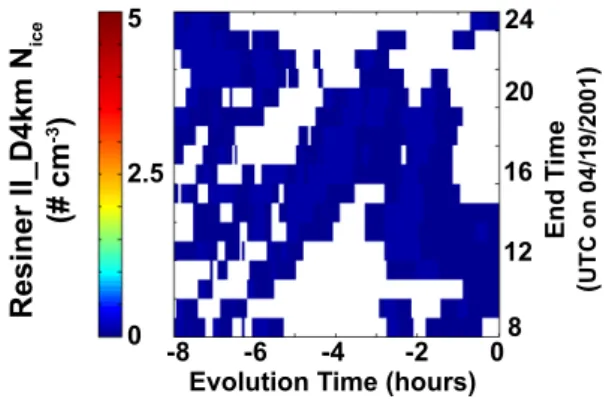
Both Nice variability and cloud lifetime variability were robust features of the parcel model Ci. In contrast, the Reis-ner II Ci had limited variability in Niceand Ci cloud evolu-tion (Fig. 11). These differences suggest that while the large-scale forcing controlled the location of Ci formation, homo-geneous freezing at locally variable w produced the modeled Niceand Ci evolution variability.

Because changes along individual or even hourly trajecto-ries are not necessarily representative of overall changes, we statistically assessed the influence of mesoscale w variability and NI Nspecification on parcel model Ci by comparing P(σ ) and P(Nice) calculated along all 266 Lagrangian trajectories.

-8 -6 -4 -2 0 Evolution Time (hours)

R es in er II _D 4k m Nic e (# c m -3) 8 24 En d Ti m e ( U TC o n 04 /1 9/ 20 01 ) 12 16 20 5 0 2.5

Fig. 11. Reisner II Ci along hourly trajectories: N_ice generated

by the Reisner II microphysical scheme in MM5 D4km are plotted along trajectories ending 12 km above Lamont. White indicates no cloud was present (IWC <0.01 mg m−3). See Fig. 9 for a descrip-tion of time-time plots.

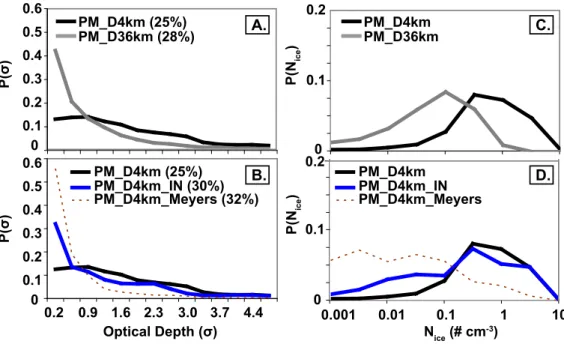
Comparison between P(σ ) and P(Nice) derived along all of the D36km and D4km trajectories illustrates the influence of mesoscale w variability and w amplitude on Ci proper-ties (Fig. 12). Along D4km trajectories, large w associated with mesoscale w variability broadened P(σ ) and shifted P(Nice) towards large values. Given that large Nice lead to long τfalloutand long cloud lifetimes, we expected more cloud cover along the D4km trajectories than along the D36km tra-jectories. We found the opposite: D4km trajectories had 3% less cloud cover than D36km trajectories. Owing to their dif-fering spatial resolutions, the D36km and D4km domains had different representations of the large-scale cooling and grav-ity wave evolution in the lee of the Rockies. Indeed, both the amplitude and the frequency structure of Lagrangian w var-ied with the spatial resolution of the MM5 domain (Fig. 6). In the end, our analysis could not isolate the influence of mesoscale w variability on cloud lifetimes and cloud cover from these systematic differences related to the spatial reso-lution of the resolved dynamics.

Adding NI N to parcels increased Ci cloud cover along the Lagrangian trajectories from 25% (NI N=0) to 30% for background NI N and to 32% for Meyers et al. (1992) NI N (Fig. 12). This cloud cover increase occurred only for op-tically thin Ci and resulted because heterogeneous freezing occurred at a lower RHice than homogeneous freezing (see Table 3).

The impact of IN on optically thick Ci depended on NI N. Due to scavenging and their relatively low concentrations, background IN had little impact on the large σ and large Nice Ci that formed by homogeneous freezing. In contrast, the use of the Meyers et al. (1992) parameterization resulted in a large addition of NI N to parcels and a decrease in the occurrence of large Nice and large σ Ci. The Meyers et al. (1992) parameterization produced more IN than are typically observed in the upper troposphere (Meyers NI N>0.3 cm−3). Therefore, we suggest that our background NI N modeling

results are more likely to represent the typical influence of IN on Ci.

5.4 Comparison of modeled and observed Ci

Both the parcel model and Reisner II scheme reproduced the observed orographic Ci formation in the lee of the Rockies; however, both models failed to reproduce the observed Ci presence above Lamont. The lidar depolarization showed Ci occurring continuously from 08:00 to 24:00 UTC (Fig. 1), yet both the parcel model (Fig. 10) and Reisner II (Fig. 11) produced no Ci above Lamont after 16:00 UTC.

Differences between modeled and observed horizontal ad-vection may have contributed to a lack of modeled Ci pres-ence above Lamont. At a height of 12 km, the MM5 horizon-tal wind speeds were up to 10 m s−1 _{smaller than observed} horizontal wind speeds (Fig. 7). For a fixed Ci cloud life-time, increasing the horizontal wind speed could alter oro-graphic Ci presence above Lamont. For example, an increase in model advection speeds may have allowed parcel model Ci to persist farther from the Rockies and to arrive above La-mont from 16:00 to 20:00 UTC (Fig. 10). Yet, horizontal advection speed cannot entirely explain differences between observed and modeled Ci presence. The GOES observations indicate that Ci persisted after passing above Lamont (Fig. 1). A moisture deficit could explain the differences between the modeled and observed Ci presence. Modeled RHice above Lamont were <100% after 15:00 UTC, which pro-moted sublimation of the orographic Ci and inhibited new freezing events (Fig. 13). Low RHiceresulted from net subsi-dence (warming) in the two hours before trajectories arrived at Lamont (Fig. 9). The model moisture deficit could have re-sulted because the MM5 forecast did not adequately capture warm frontal lifting throughout the South Central USA. The reduced southern extent of Montana low in the MM5 forecast as compared to the NWS reanalysis supports this hypothesis. Given modeled RHice<100%, it is not surprising that few model Ci arrived at Lamont. With modeled RHice>100%, more orographic Ci may have survived and arrived at Lam-ont. In addition, only modest lifting is required for parcels near ice saturation to reach a homogeneous freezing thresh-old. If model parcels were lifted an additional 300 to 400 m, new homogeneous freezing events could have occurred and

w variability could have resulted in variable Nice.

Despite obvious differences between the observed and modeled Ci presence, model Ci did form in the lee of the Rockies and were advected to Lamont (Figs. 10, 11). By comparing the observed and modeled Ci properties (Table 4), we found that the parcel model helped explain the Ci obser-vations in the following ways:

1. Observed 1Z variability clearly contributed to the ob-served broad P(σ ) (Fig. 2); however, the obob-served broad P(σ ) at Lamont (Fig. 2) could also be partially explained by variable Nice resulting from homogeneous freezing

0 0.1 0.2 0.3 0.4 0.5 0.6 P( σ) P( Nice ) 0 0.1 0.2 A. C. Optical Depth (σ) P( Nice ) 0 0.1 0.2 B. 0.2 0.9 1.6 2.3 3.0 3.7 4.4 N_ice (# cm-3₎ 0.001 0.01 0.1 1 10 D. PM_D4km (25%) PM_D4km_IN (30%) PM_D4km_Meyers (32%) PM_D4km PM_D4km_IN PM_D4km_Meyers 0 0.1 0.2 0.3 0.4 0.5 0.6 P( σ) PM_D4km (25%) PM_D36km (28%) PM_D4kmPM_D36km

Fig. 12. Influence of MM5 domain resolution and IN parameterization on parcel model P(σ ) and P(Nice). P(σ ) and P(Nice) were calculated

along trajectories ending 12 km above Lamont from 12:00 to 24:00 UTC. The cloud fraction (cf) is listed after the parcel model experiment name. Cloudy air must have an IWC>0.01 mg m−3_{. P(N}

ice) were calculated for Nice>0.001 cm−3. P(σ ) were calculated for σ >0.1. The

Meyers P(σ ) and P(Nice) are dashed because the Meyers et al. (1992) parameterization resulted in NI Nthat are not atmospherically relevant.

See Table 3 for parcel model experiment details and naming conventions.

210 211 212 213 214 215 216 217 218 219 220 8 12 16 20 Hour (UTC) on 04/19/2001 Te m pe ra tu re (K ) 0 20 40 60 80 100 120 140 24 R H ic e (% )

Fig. 13. Model humidity and temperature 12 km above Lamont:

Both the parcel model (PM D4km, solid lines) and the Reisner II scheme (ReisnerII D4km, dotted lines) air at Ci levels above Lam-ont was sub-saturated with respect to ice.

at variable w. Although the modeled P(σ ) (Fig. 12) are not coincident in time and space with the P(σ ) observa-tions at Lamont, broad modeled P(σ ) along trajectories resulted from homogeneous freezing occurring at vari-able w.

2. Large Niceresulted in long parcel modeled Ci lifetimes. Thus, the parcel model could help explain the observed persistence of Ci over many hours in the GOES imagery.

Table 4. Model vs. observed variability in Ci properties above

Lamont from 08:00 to 24:00 UTC on 19 April 2001. Model values are only included for model IWC>0.01 m m−3_.

Source Nice Reff σ

cm−3 µm dimensionless PM D4km 0.01–3.05 1–25 0.01–2.3 PM D4km IN 0.01–2.71 6-30 0.01–2.3 PM D4km Meyers 0.001–1.04 5–25 0.01–1.1 ReisnerII D4km 0.02–0.08 25–36 NA Observed NA NA 0–3 6 Conclusions

Using self-consistent Lagrangian trajectories derived from a mesoscale weather model and an adiabatic parcel model with binned ice microphysics, this study evaluated the influence of mesoscale w and IN presence on Ci Nice, and inhomogeneity during an orographic Ci case study. The primary findings were:

– When mesoscale variability (along-path fluctuations

with timescales of 2 h−1_{<ν<10 h}−1_{) in w affected} ho-mogeneous freezing, P(σ ) derived along Lagrangian trajectories were broad. Broad P(σ ) resulted because homogeneous freezing driven by variable w led to variable Nice, variable σ , and variable Ci lifetimes.

– The addition of IN to air parcels increased cloud cover

along Lagrangian trajectories by 5 to 7%, depending on the NI N and IN freezing threshold. Whereas back-ground NI N (NI N=0.03 cm−3) presence had little in-fluence on the occurrence of large σ , the presence of large NI N(NI N>0.3 cm−3), resulting from use of Mey-ers et al. (1992) parameterization, decreased the occur-rence of large σ by suppressing homogeneous freezing. Because the Meyers et al. (1992) parameterization pro-duced more IN than are typically observed in the up-per troposphere (NI N<0.1 cm−3(DeMott et al., 2003; Rogers et al., 1998)), the background NI N modeling results are representative of what occurs in the atmo-sphere.

– All models predicted fewer Ci than were observed. Low

humidities along modeled trajectories, which were at-tributed to a lack of MM5 frontal lifting, could explain differences in modeled and observed Ci. Nevertheless, the parcel model Ci helped explain observed Ci inho-mogeneity in the following sense: 1) Broad observed P(σ ) could be partially explained by variable Nice ar-riving along parcel model Ci trajectories, 2) Large Nice predicted by the parcel model resulted in long Ci life-times and could explain the persistence of Ci over many hours.

Although there are limitations associated with using an adia-batic parcel model and trajectories to represent Ci processes and properties, the results from this study demonstrate clear connections between mesoscale w, Ci Nice, and Ci P(σ ). Our results support and extend the results of K¨archer and Str¨om (2003); Hoyle et al. (2005); Haag and K¨archer (2004), who suggested that w variability and homogeneous freezing gen-erate Nicevariability in the atmosphere.

The primary goal of this study was to illustrate the influ-ence of mesoscale w and NI N variability on Ci P(σ ) along numerous realistic Lagrangian trajectories. Therefore, we were not alarmed to find deviations between modeled and observed Ci presence. A mesoscale model forecast is an ini-tial value problem with a single realization. We could have generated MM5 forecasts until we reproduced the observed Ci presence, but a detailed reproduction of the observations was not our goal. The observations were invaluable because they helped us identify 19 April 2001 as a good case study, not because they provided a benchmark for evaluating the ability of models to exactly reproduce observations.

Given the limitations of this study, and that this is only a single case study, the influence of w and IN on Ci cloud prop-erties should be explored further. In particular, modeling Ci evolution along trajectories derived from models that resolve

w variability at small spatial scales (ν>6 h−1_{) would be}

use-ful. In addition, including the effects of variable 1z on Ci P(σ ) and comparing the influence of 1z with the influence of w highlighted by this study would be interesting. It is im-portant to note that using a more complex model to assess the

influence of 1Z variability on σ variability requires an accu-rate vertical moisture profile. Finally, we recommend inves-tigation of the parallels between the w-Nice-cloud lifetime-cloud cover connections described in this study and the in-direct effects of aerosols on stratus albedos, lifetimes, and cloud cover (e.g. Twomey, 1974; Albrecht, 1989).

Acknowledgements. We acknowledge NSF-ATM-02-1147 for

research funding and the NCAR Scientific Computing Division for providing computing resources. J. E. Kay was supported in part by the Office of Biological and Environmental Research of the U.S. Department of Energy under contract DE-AC06-76RL01830 to the Pacific Northwest National Laboratory as part of the Atmospheric Radiation Measurement Program. The Pacific Northwest National Laboratory is operated by Battelle for the U.S. Department of Energy. We thank T. Ackerman, Q. Fu, and J. Locatelli for productive scientific discussions, D. Turner for providing and helping to interpret the Raman lidar observations, and M. Stoelinga and D. Durran for help with the MM5 simulations. Edited by: B. K¨archer

References

Albrecht, B.: Aerosols, cloud microphysics and fractional cloudi-ness, Science, 245, 1227–1330, 1989.

Carlin, B., Fu, Q. Lohmann, U., Mace, G., Sassen, K., and Com-stock, J.: High-cloud horizontal inhomogeneity and solar albedo bias, J. Clim., 15(17), 2321–2339, 2002.

Dean, S. M., Lawrence, B. N., Grainger, R. G. and Heuff, D. N.: Orographic cloud in GCM: the missing cirrus, Clim. Dyn., 24, 771–780, 2005.

DeMott, P. J., Cziczo, D. J., Prenni, A. J., Murphy, D. M., Krei-denweis, S. M., Thomson, D. S., Borys, R., and Rogers, D. C.: Measurements of the concentration and composition of nuclei for cirrus formation, Proc. Natl. Acad. Sci., 100(25), 14 655–14 660, 2003.

Durran, D. R.: Lee Waves and Mountain Waves, in: Encyclope-dia of Atmospheric Science, edited by: Holton, J., Pyle, J., and Curry, J., Academic Press, 2003.

Field, P. R., Cotton, R. J., Noone, K., Glantz, P., Kaye, P. H., Hirst, E., Greenaway, R. S., Jost, C., Gabriel, R., Reiner, T., Andreae, M., Saunders, C. P. R., Archer, A., Choularton, T., Smith, M., Brooks, B., Hoell, C., Bandy, B., Johnson, D., and Heymsfield, A.: Ice nucleation in orographic wave clouds: Measurements made during INTACC, Q. J. Roy. Meteor. Soc., 127(575), 1493– 1512, 2001.

Fu, Q., Carlin, B., and Mace, G.: Cirrus horizontal inhomogeneity and OLR bias, Geophys. Res. Lett., 27(20), 3341–3344, 2000. Grell, G. A., Dudhia, H., and Stauffer, D. R.: A description of

the fifth generation Penn State NCAR Mesoscale Model (MM5), NCAR Tech Note NCAR/TN-398+STR, National Center for At-mospheric Research (NCAR), Boulder, CO, 121 pp., 1994. Haag, W. and K¨archer, B.: The impact of aerosols and gravity waves

on cirrus clouds at mid-latitudes, J. Geophys. Res., 109, D12202, doi:10.1029/2004JD004579, 2004.

Heymsfield, A. J. and Miloshevich, L.: Relative Humidity and Tem-perature Influences on Cirrus Formation and Evolution:

Obser-vations from Wave Clouds and FIRE II, J. Atmos. Sci., 52, 4302– 4326, 1995.

Hoyle, C. R., Luo, B. P., and Peter, T.: The origin of high ice crystal number densities in cirrus clouds, J. Atmos. Sci., 62, 2568–2579, 2005.

K¨archer, B. and Lohmann, U.: A parameterization of cirrus cloud formation: heterogeneous freezing, J. Geophys. Res., 108, D14, doi:10.1029/2002JD003220, 2003.

K¨archer, B. and Str¨om, J.: The roles of dynamical variability and aerosols in cirrus cloud formation, Atmos. Chem. Phys., 3, 823– 838, 2003,

http://www.atmos-chem-phys.net/3/823/2003/.

Kay, J. E.: Physical controls on cirrus cloud inhomogeneity, Ph.D. Thesis, University of Washington, 2006.

Kay, J. E., Baker, M., and Hegg, D.: Microphysical and dynamical controls on cirrus cloud optical depth distributions, J. Geophys. Res., 111, D24205, doi:10.1029/2005JD006916, 2006.

Koop, T., Luo, B., Tslas, A., and Peter, T.: Water activity as the de-terminant for homogeneous ice nucleation in aqueous solutions, Nature, 406, 611–614, 2000.

Mace, G. G., Clothiaux, E. E., and Ackerman, T. P.: The composite characteristics of cirrus clouds: bulk properties revealed by one year of continuous cloud radar data, J. Climate, 14, 2185–2203, 2001.

Meyers, M. P., DeMott, P. J., and Cotton, W. R.: New primary ice-nucleation parameterization in an explicit cloud model, J. Appl. Meteorol., 55, 2039–2052, 1992.

Reisner, J., Rasmussne, R. M., and Bruintjes, R. T.: Explicit fore-casting of supercooled liquid water in winter storms using the MM5 mesoscale model, Q. J. Roy. Meteor. Soc., 124,1071–1107, 1998.

Rogers, D. C., DeMott, P. J., Kredenweis, S. M., and Chen, Y.: Measurements of ice nucleating aerosols during SUCCESS, Geophys. Res. Lett., 25(9), 1383–1386, 1998.

Turner, D. D.: Arctic mixed-phase cloud properties from AERI li-dar observations: Algorithm and results from SHEBA, J. Appl. Meteorol., 44(4), 427–444, 2005.

Twomey, S. A.: Pollution and the planetary albedo, Atmos. Envi-ron., 8, 1251–1256, 1974.