Low thrust minimum-fuel orbital transfer: a homotopic approach

HAL Id: inria-00271161

https://hal.inria.fr/inria-00271161

Submitted on 8 Apr 2008

HAL is a multi-disciplinary open access

archive for the deposit and dissemination of sci-entific research documents, whether they are pub-lished or not. The documents may come from teaching and research institutions in France or abroad, or from public or private research centers.

L’archive ouverte pluridisciplinaire HAL, est destinée au dépôt et à la diffusion de documents scientifiques de niveau recherche, publiés ou non, émanant des établissements d’enseignement et de recherche français ou étrangers, des laboratoires publics ou privés.

Low thrust minimum-fuel orbital transfer: a homotopic

approach

Thomas Haberkorn, Pierre Martinon, Joseph Gergaud

To cite this version:

Thomas Haberkorn, Pierre Martinon, Joseph Gergaud. Low thrust minimum-fuel orbital transfer: a homotopic approach. Journal of Guidance, Control, and Dynamics, American Institute of Aeronautics and Astronautics, 2004, 27 (6), pp.1046-1060. �inria-00271161�

Low thrust minimum-fuel orbital transfer: a

homotopic approach

T. Haberkorn

∗

, P. Martinon

†

, and J. Gergaud

‡

Abstract: We describe in this paper the study of an earth or-bital transfer with a low thrust (typically electro-ionic) propulsion system. The objective is the maximization of the final mass, which leads to a discontinuous control with a huge number of thrust arcs. The resolution method is based on single shooting, combined to a homotopic approach in order to cope with the problem of the ini-tial guess, which is actually critical for non-trivial problems. An important aspect of this choice is that we make no assumptions on the control structure, and in particular do not set the number of thrust arcs. This strategy allowed us to solve our problem (a trans-fer from Low Earth Orbit to Geosynchronous Equatorial Orbit, for a spacecraft with mass of 1500 kgs, either with or without a rendez-vous) for thrusts as low as 0.1N, which corresponds to a one-year transfer involving several hundreds of revolutions and thrust arcs. The numerical results obtained also revealed strong regularity in the optimal control structure, as well as some practically interesting em-piric laws concerning the dependency of the final mass with respect to the transfer time and maximal thrust.

∗ _{PhD student, email: thomas.haberkorn@enseeiht.fr} † _{PhD student, email: pierre.martinon@enseeiht.fr} ‡ _{Senior lecturer, email: joseph.gergaud@enseeiht.fr}

Introduction

The minimum-fuel orbital transfers, in which one aims at minimizing fuel con-sumption in order to optimize the payload, are difficult to solve, as they lead to discontinuous “switching” controls. Direct resolution methods, which typ-ically involve partial or total discretization of the problem, were predictably unsuitable for our problem, due to the huge number of resulting variables for long transfers at low thrusts. Indirect methods thus seemed more appropriate, but are known to be critically sensitive to the initial guess, which severely impairs their application to difficult problems. As a matter of fact, the single shooting method, for instance, is based on a Quasi-Newton solver, and can therefore have a very poor convergence radius, making it pretty inefficient for the chosen kind of problems if one tries to apply it directly. Indeed, the resolu-tion of such problems often requires making some a priori assumpresolu-tions about the structure of the control, and more specifically to set the number of thrust arcs (see for instance [1, 2, 3]). Yet given the results of the minimum time problem resolution, see [4, 5, 6, 7], we expected a large number of revolutions and therefore, of thrust arcs, at low thrusts, so these kinds of assumptions were not acceptable. We thus needed a method that would determine by itself the control structure, and this is why we chose to use primarily the single shooting method, despite th e critical problem of the initial guess. This paper describes the homotopic approach we used to solve this difficulty, and the numerical results we were able to obtain.

The minimum fuel orbital transfer

The problem we address here is a case of Earth orbital transfer, in which we want to move a satellite from a low, elliptic, and inclined initial orbit to an equatorial geostationary destination orbit. We originally considered a free final longitude transfer, with an unknown number of revolutions and no rendez-vous on the final orbit. To solve a rendez-vous problem, we first consider the same problem with free final longitude, which gives an accurate approximation of the number of revolutions. Then we set the final longitude according to the number of revolutions and the rendez-vous constraint to solve the problem.

One of the main difficulties is that we consider low thrust transfers (typi-cally involving electro-ionic propulsors), which implies long transfer times and a great number of revolutions (up to several hundreds for a one-year transfer with a thrust of 0.1N). The initial and arrival orbits are shown in Figure 1.

Figure 1: Orbital transfer

Note: The third graph showing inclination has been rescaled for better vis-ibility. The initial orbit is actually slightly inclined (about 7 degree) above the equatorial plane. A simplified version of the full 3-dimensional transfer is the coplanar transfer, where both control and trajectories remain in the equatorial plane. We actually began experimentations with this 2D transfer.

The satellite is subject only to Earth gravitational forces (1/r2 _{first term}

only approximation) and the thrust of its own propulsion system, the lat-ter being the control of our problem. Solving the optimal control problem thus consists in determining the best thrust command law with respect to the objective. The minimun time transfer problem has already been extensively studied, see [4, 5, 6, 7], and we seek here to minimize fuel consumption dur-ing the transfer. The choice of this criterion, which we will refer to as the “minimum fuel” or “maximal mass” problem, leads to a discontinuous control, with a huge number of switches and thrust arcs for low thrusts, as we shall see.

Problem statement

Our state vector consists of the position, speed and mass of the satellite at a given time t. It is of course possible to express the position and speed in a geocentric cartesian system, yet according to the expected high number of revolutions, this would lead to strong oscillations, which is detrimental to nu-merical stability. This is why we prefer to use a modified set of classical orbital elements, which describes the movement of the satellite in a more orbit-related point of view. There we use the first five components of the state vector to char-acterize the osculating orbit (the orbit the satellite would follow if no thrust was applied), while the sixth component indicates the current position of the satellite on this orbit. As the orbit deformation is quite smooth, especially for low thrust transfers, this guarantees a very good numerical stability for our state vector, which would not be the case with the cartesian expression. This

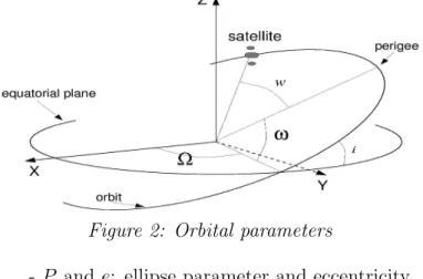
particular choice of coordinates is illustrated on Figure 2:

Figure 2: Orbital parameters with

- P and e: ellipse parameter and eccentricity - θ: true anomaly

- Ω: ascending node longitude - ω: argument of perigee - i: inclination

Let us now define our state variables in R7

: • Orbit parameter P

• Eccentricity vector (ex, ey), in the orbit plane, oriented towards perigee

• Rotation vector (hx, hy), in the equatorial plane, colinear to the

intersec-tion of orbit and equatorial planes • True longitude L

According to the previous notations, these parameters are defined as:

ex = e cos (Ω + ω) , ey = e sin (Ω + ω)

hx = tan(i/2)cosΩ , hy = tan(i/2)sinΩ

L = Ω + ω + θ

As for the three-dimensional control, we choose to express it in the moving reference frame attached to the satellite, as shown on Figure 3.

Figure 3: Control expression

The normalized control u (such as the thrust −−→T (t) = u(t) Tmax) is thus

expressed in R3

as: radial thrust q, transverse thrust s and normal thrust w.

Remark: in the case of the simplified coplanar transfer, one just has to sup-press components (hx, hy) in the state and component w in the control, which

deal with the inclination of the orbits.

Here are the initial and terminal conditions of our problem:

At t0 = 0 At tf

• P = 11625 Km • P = 42125 Km • (ex; ey) = (0.75; 0) • (ex; ey) = (0; 0)

• (hx; hy) = (0.0612; 0) • (hx; hy) = (0; 0)

• L = π • f ree f inal longitude • m = 1500 Kgs • f ree f inal mass

Note: it should be mentioned that the free final longitude problem, of a rather theoretical interest, is actually more difficult to solve than the fixed final longitude transfer, mainly due to the presence of local solutions. As a matter of fact, the resolution of this problem is attained via the resolution of fixed longitude problems, which are practically easier to solve, as we shall see.

If we note TM ax the maximal thrust and Isp the specific impulse of the

pro-peller, the chosen approximation of gravitational forces leads to the following dynamics of the problem:

                                                                               ˙ P (t) = 2TM ax m(t) q P3 (t) µ0 s(t) Z(t) ˙ex(t) = T_m(t)M ax q P(t) µ0 1 Z(t)[Z(t)sin(L(t))q(t) + A1(t)s(t)

−ey(t)(hx(t)sin(L(t)) − hy(t)cos(L(t)))w(t)]

˙ey(t) = T_m(t)M ax q P(t) µ0 1 Z(t)[−Z(t)cos(L(t))q(t) + A2(t)s(t) +ex(t)(hx(t)sin(L(t)) − h)y(t)cos(L(t)))w(t)] ˙hx(t) = T_2m(t)M ax q P(t) µ0(t) X(t) Z(t)cos(L(t)).w(t) ˙hy(t) = T_2m(t)M ax q P(t) µ0(t) X(t) Z(t)sin(L(t)).w(t) ˙L(t) =q _µ 0 P3 (t)Z 2_{(t) +} 1 m(t) q P(t) µ0 × _Z(t)1 (hx(t)sin(L(t)) − hy(t)cos(L(t)))w(t) ˙ m(t) = −TM ax Ispg0 k(q(t), s(t)), w(t)k W ith        Z(t) = 1 + ex(t) cos(L(t)) + ey(t) sin(L(t)) A1(t) = ex(t) + (1 + Z(t)) cos(L(t)) A2(t) = ey(t) + (1 + Z(t)) sin(L(t)) X(t) = 1 + h2 x(t) + h2y(t)

If we note x = (P, ex, ey, hx, hy, L) and u = (q, s, w) we obtain the following

formulation of our maximal mass orbital transfer problem:

(Pmf)                          M ax m(tf) ˙x(t) = a(x(t)) + TM ax m(t)B(x(t))u(t) , ∀t ∈ [t0, tf] ˙ m(t) = −TM ax Ispg0 ku(t)k ku(t)k ≤ 1, ∀t ∈ [t0, tf] IC : x(t0) = (11625; 0.75; 0; 0.0612; 0; π; 1500) T C : x(tf) = (42165; 0; 0; 0; 0; f ree; f ree) t0 = 0 tf = tfM in. ctf

Contrary to minimum-time problems, in which the transfer time is the ob-jective to be minimized, and thus the final time tf is free, we consider here a

fixed time transfer. The reason for this choice is that it is not obvious that the minimum fuel problem with free final time has a solution. To set the value of the transfer time tf, we first solve the minimum-time transfer problem, with

which the transfer is not feasible. Then we set tf to a certain multiple of tfM in,

ie:

tf = tfM in.ctf , with ctf > 1

Besides, the actual criterion used for the maximization of the payload is not

M ax m(tf) but M in

Z tf

t0

ku(t)kdt which is equivalent per the mass dynamic:

˙

m(t) = −TM ax

Ispg0 ku(t)k

Single shooting difficulties

We primarily use to solve this problem the single shooting method (based on Pontryagin’s Maximum Principle), which transforms an optimal control problem to solving an equation of the form S(z) = 0, where S is the shooting function associated with the original problem. This method is part of the class of indirect methods, by opposition to direct methods, where the problem is solved for instance via discretization and sequential quadratic programming (SQP). One of the main advantages of this approach is that we do not have to make any assumptions regarding the structure of the control: the number of switches in thrust level and direction, in particular, is not set a priori.

Yet a major drawback of this class of methods is that they require a good initial guess: as they typically consist in applying a Quasi-Newton solver to the shooting function, the convergence radius may be quite small, depending on the problem. And unless the dimension of the search space is extremely low, it is not realistic to explore it randomly to find a suitable initial point. This is why we will use a homotopic approach, but let us begin with the presentation of the single shooting method.

We introduce the costate (p, pm) with p = (pP; pex; pey; phx; phy; pL), and

then define the Hamiltonian H(t, x, m, p, pm, u):

H(t, x, m, p, pm, u) = ku(t)k + (p(t)| ˙x(t)) + (pm(t)| ˙m(t))

which for our problem gives:

H(t, x, m, p, pm, u) = (1 − T_IspM ax_g0pm(t)) ku(t)k

+ TM ax

m(t)(B(x(t))u(t)|p(t)) + (a(x(t))|p(t))

Then the application of Pontryagin’s Maximum Principle and optimality necessary conditions gives the expression of the optimal control, or H-minimal command, which minimizes the Hamiltonian H:

ψ(t, x, m, p, pm) = 1 − T_IspM ax_g0 pm(t) − T_m(t)M axkBt(x(t))p(t)k

Then we have the following expression of the control

     u(t) = −_kBBtt(x(t))p(t)_(x(t))p(t)k if ψ(t, x, m, p, pm) < 0 u(t) = −α_kBBtt(x(t))p(t)_(x(t))p(t)k α ∈ [0, 1] if ψ(t, x, m, p, pm) = 0 u(t) = 0 if ψ(t, x, m, p, pm) > 0 Else if Bt_{(x(t))p(t) = 0 we have}      u(t) ∈ S(0, 1) if 1 −TM ax Ispg0 pm(t) < 0 u(t) ∈ B(0, 1) if 1 −TM ax Ispg0 pm(t) = 0 u(t) = 0 if 1 −TM ax Ispg0 pm(t) > 0

We can see that this control can be discontinuous, as its norm switches between 0 and 1 at zeros of the switching function ψ.

We now make two assumptions, which will be numerically verified:

(H1) We assume that Bt_{(x(t))p(t) is non-zero for all t ∈ [t} 0, tf]

(H2) There is no singular arc, that is to say that we do not have ψ(t, x, m, p, pm) = 0 on any finite interval.

Even under these assumptions, the application of the single shooting can be quite tricky, which is in particular due to the fact that the control structure is not known a priori. We will now detail the resolution of a simple example, both to point out some of the difficulties that can be expected to arise with our orbital transfer, and to illustrate the different steps of our method.

Illustration on a simple example

Let us consider the following optimal control problem:

(P2)                        M in R2 0 |u(t)|dt ˙x1(t) = x2(t) ˙x2(t) = u(t) |u(t)| ≤ 1 x1(0) = 0 x2(0) = 0 x1(2) = 0.5 x2(2) = 0

The corresponding Boundary Value Problem is: (BV P2)                ˙x1(t) = x2(t) ˙x2(t) = u(t) ˙p1(t) = 0 ˙p2(t) = −p1(t) x(0) = x0 x(2) = xf

And the optimal control, which minimizes the Hamiltonian H : (t, x, p, u) 7→ ku(t)k + p1(t)x2(t) + p2(t)u(t), is given by:

  

u(t) = −sgn(p2(t)) if |p2(t)| > 1

u(t) = 0 if |p2(t)| < 1

u(t) = α p2(t) with α ∈ [0, 1] otherwise

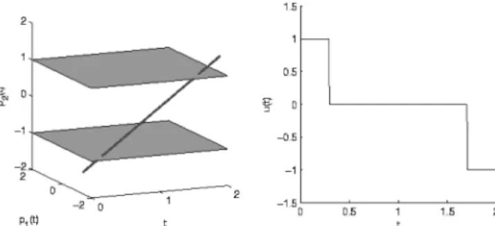
So we have a discontinuous control, whose norm switches between 0 and 1 when |p2(t)| = 1, as shown below on Figure 4:

Figure 4: Costate and Optimal control at the solution for (P2)

If we examine the possible values of the initial costate (p1(0), p2(0)) in R2,

we can see that the costate dynamics and optimal control expression lead to 9 different possible optimal control structures, which are here represented on Figure 5:

Figure 5: Control structures for (p1(0), p2(0)) in R2

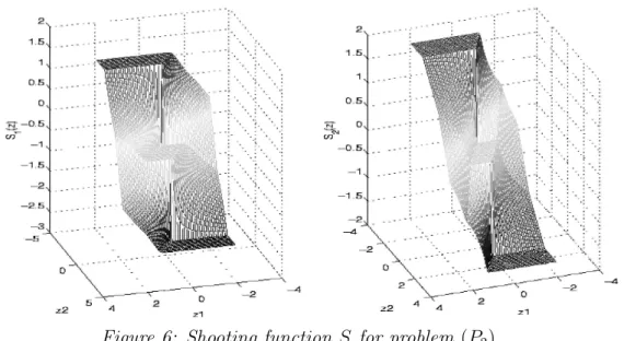
We define the shooting function:

S(z) = x(2; x0, z) − xf

where x(2; x0_{, z) is the solution of the following Initial Value Problem:}

(IV P2)                ˙x1(t) = x2(t) ˙x2(t) = u(t) ˙p1(t) = 0 ˙p2(t) = −p1(t) x(0) = x0 p(0) = z

Solving the original problem (P2) by the shooting method thus consists of

solving the equation S(z) = 0. Figure 6 represents S, and permits recognition of the 9 previously mentioned regions :

Figure 6: Shooting function S for problem (P2)

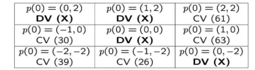
It must be pointed out that S is not differentiable on the boundaries of these domains, and is not even defined in (0, −1) and (0, 1). Thus difficulties are to be expected when trying to solve S(z) = 0 with a Newton-like algorithm, especially if the initial guess does not lie in the correct domain. And actually, even in this very simple case, trying to solve directly S(z) = 0 from a random initial point is non trivial, as we can see on Table 1 (indicated in parenthesis is the number of iterations performed by the solver):

Table 1: (P2) Single Shooting results for various initial points

(CV(iterations) indicates convergence and DV(X) divergence)

Of course, here there are only a few regions to explore, and convergence may even be attained from an initial point in the “wrong” region (at an increased iteration cost), but this is due to the simplicity of problem (P2).

The shooting functions related to the orbital transfer problems, on the other hand, tend to be numerically unstable and require careful handling to avoid troubles. In particular, the value of S is computed through the integration of a problem with a discontinuous right hand side, which becomes increasingly difficult as the number of switches grows (typically for low-thrust transfers). This integration can actually lead to numerical aberrations for certain values of the initial costate p(0), such as negative orbit parameter or eccentricity, and the shooting function is thus not defined on the whole search space. More-over it is critical to keep an eye on the precision of this evaluation, especially as we will have to approximate the Jacobian of S (see the description of the PC continuation method below). We use for this a standard centered finite differences method, whose steplength must be set according to the precision with respect to S. For instance, taking a too small steplength leads to an erroneous approximation of the Jacobian, which severely impairs convergence, or can even cause divergence.

These difficulties make it actually nearly impossible to find a solu-tion of S(z) = 0 without a very close initial guess. A possible workaround for this is to solve first the problem for a high thrust (say 60N), which is much easier, and use this solution as an initial guess to try to solve the problem with a lower thrust. This sequential approach, that we call “discrete continuation” was actually used with success for the minimum time transfers (cf [5]), but failed for our maximum mass problems, which is why we used a homotopic method.

Homotopic method

Basically, the principle of a homotopic approach is to solve a difficult problem by starting from the known solution of a somewhat related, but easier problem. By related we mean that there must exist an application H, called a homotopy, with the right properties connecting the two problems.

Let r and f be two applications from Rn _{into R}n_{. We shall call an}

H : Ω × [0, 1] → Rn

(z, λ) 7→ H(z, λ)

with Ω a bounded open set in Rn _{and H continuous, so that}

H(., 0) = r H(., 1) = f

The first task is thus to find such a proper application H for our orbital transfer problem. In our case, while maximizing the final mass leads to a diffi-cult problem, due to the discontinuous nature of the optimal control, changing the objective into the minimization of the energy (M in Rtf

t0 ku(t)k

2 _{dt) gives}

a much more regular problem, with a continuous control.

A convenient way to build a suitable homotopy H connecting these two problems is to consider a homotopic criterion linking the mass criterion (when λ = 1) and the energy criterion (when λ = 0). Thus the shooting function associated with this modified problem can be taken as the homotopy H. So we define a homotopy connecting these two problems, mass maximization and energy minimization, by using one of these two homotopic criteria (others were of course possible):

Z tf

t0

λku(t)k + (1 − λ)ku(t)k2 dt (convex criterion) or

Z tf

t0

ku(t)k2−λ dt (power criterion)

It is clear that we have in λ = 0 the energy problem and in λ = 1 the mass problem. The point is that this energy problem is indeed much easier to solve than the mass problem, with a much better convergence radius for the shooting method. Now, provided we have a solution of the energy problem, i.e., a zero of H(., 0), all we have to do is to follow the zero path of H until we reach a zero of H(., 1), i.e., a solution of our mass problem.

Let us apply this to our simple example (P2). For the minimization of the

energy, we have the optimal control:

½ u(t) = −sgn(p2(t)) if |p2(t)| ≥ 2

u(t) = −p2(t)/2 otherwise

Contrary to the mass problem, the single shooting converges here for an initial guess in any of the previously seen nine domains. The following graph (Figure 7) shows the zero path of the homotopy H, and the evolution of the op-timal control from the previous smooth expression to a discontinuous structure (for the mass criterion).

Zero Path Following

There are different ways to achieve this zero path following, among which we tried three different classes: the discrete continuation methods, the Piecewise Linear (PL) continuation methods, and the Predictor Corrector (PC) contin-uation methods. We shall now briefly describe the principles of these methods to present their respective advantages and drawbacks. Readers interested in these methods should refer in particular to [9, 10], where these algorithms are thoroughly detailed.

Discrete continuation

The simplest way to follow the zero path of the homotopy is basically to try to solve a sequence of equations of the form H(z, λ) = 0, with λ growing from 0 to 1, by taking the previously obtained solution as an initial guess for the next try. This method actually involves no real path following (the question of the step in λ, in particular, is left to the experimenter), and is a rather marginal approach, which can hope to converge to a solution of f (z) = 0 in easy cases only.

Piecewise Linear (PL) methods (simplicial methods)

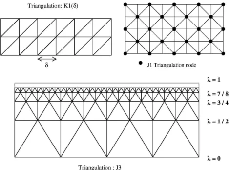
PL continuation methods actually follow the zero path of the homotopy H by building a piecewise linear approximation of H, hence their name. Towards this end, the search space is subdivided into cells, most often in a particular way called a triangulation in simplices. This is why PL continuation methods are often referred to as simplicial methods. The main advantage of this ap-proach is that it puts extremely low requirements on the homotopy H: as no derivatives are used, continuity is in particular sufficient, and should not even be necessary in all cases. The main drawback of this low-level exploitation of the homotopy properties is that PL algorithms are slower than PC algorithms (see below), when the latter converge. This is strongly due to the lack of path direction prediction and the difficulty to adapt the triangulation meshsize to the followed path.

Here is a brief summary of how a simplicial algorithm follows the zero path of the homotopy. Let us begin with some useful definitions:

Simplex and Face: we call simplex the convex hull of n + 1 affinely inde-pendent points (called the vertices) in Rn_{, while a k-face of a simplex is the}

convex hull of k vertices of the simplex, as shown on Figure 8.

Triangulation: a countable family T of simplices of Rn _verifying:

• The intersection of two simplices of T is either a face or empty

• T is locally finite (a compact subset of Rn _{meets finitely many simplices).}

The Figure 9 shows some classical triangulations.

Figure 9: Illustration of triangulations K1,J1 and J3 in R2

Labeling: we shall call labeling a map l that associates a value to the ver-tices vi of a simplex. Here the simplices will be labeled by the homotopy H:

l(vi_{) = h(z}i_{, λ}i_{), where v}i _{= (z}i_{, λ}i_{). Affine interpolation on the vertices thus}

gives a PL approximation HT of H.

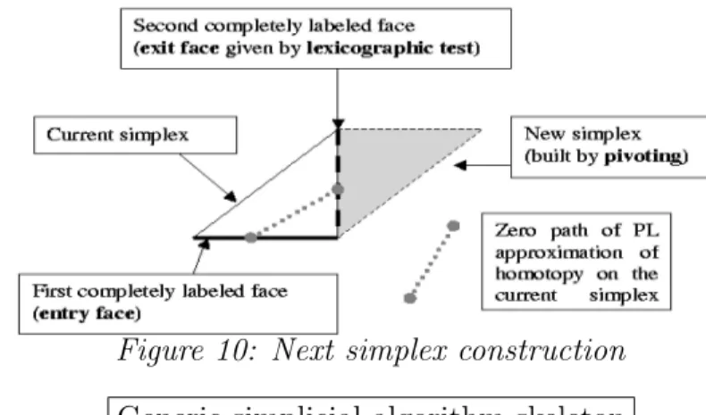
Completely labeled face: a face of a simplex is completely labeled if it con-tains a zero of the PL approximation of the homotopy H, this property being stable under certain small perturbations.

Fundamental property: each simplex possesses either zero or exactly two completely labeled faces (being called a transverse simplex in the latter case). There is a constructive proof of this property, which gives the other completely labeled face of a simplex that already has a known one. This step will be called the lexicographic test. Then there exists a unique transverse simplex that shares this second completely labeled face, that can be determined via pivot-ing rules. These two steps are shown on Figure 10:

Figure 10: Next simplex construction Generic simplicial algorithm skeleton • Start: λ = 0

First simplex with its completely labeled entry face given • Follow zero path:

While λ 6= 1 Do Lexicographic test:

Find the other completely labeled face (”exit face”) of the current simplex. Pivoting step:

Build the other simplex sharing this face with the current simplex, which be-comes the new current simplex.

Updates:

Current simplex number, inverse of labeling matrix and solution. End While

• End: retrieve the coordinates of the zero of HT when λ = 1.

A simplicial algorithm thus basically follows from λ = 0 to λ = 1 a sequence of transverse simplices, which under the right assumptions on H is finite and does not cycle. Figure 11 illustrates this generic PL algorithm:

Figure 11: Zero Path following

Predictor-Corrector (PC) method

For a more detailed explanation of the PC method, see ref. [9].

Zero path existence

Theorem :

Set Ω an open bounded subset of Rn_{. Set H : ¯Ω × [0, 1] → R}n_continuously

differentiable ( ¯Ω is the adherence of Ω) and such that :

(a) ∀(z, λ) ∈ {(z, λ) ∈ Ω × [0, 1] such that H(z, λ) = 0} the Jacobian matrix H′ _{= [}∂H ∂z1... ∂H ∂zn ∂H ∂λ] is of full rank n.

(b) ∀z ∈ {z ∈ Ω such that H(z, 0) = 0} ∪ {z ∈ Ω such that H(z, 1) = 0} the matrix [∂H

∂z1..

∂H

∂zn] is of full rank n.

Then {(z, λ) ∈ Ω × [0, 1] such that H(z, λ) = 0} is made of : (i) a finite number of closed curves (of finite length) in ¯Ω × [0, 1].

(ii) a finite number of arcs (of finite length) having their terminal points in ∂Ω × [0, 1].

Curves (i) and (ii) are separated and continuously differentiable.

Proof : see [12]

Figure 12 shows some possible and impossible paths.

possible paths impossible paths Figure 12: Possible and impossible paths

Zero path following

Let us assume that the considered homotopy (H(z, λ)) is sufficiently regular (C2_{) and that the zero path that comes from (z}

0, 0) is a differentiable curve C.

We can parametrize this curve by the curvilinear abscissa s and suppose we have the relation :

     (i) k(∂z ∂s, ∂λ ∂s)k = 1 (ii) H(z(s), λ(s)) = 0

(iii) H′_{(z(s), λ(s)) if of full rank n}

Differentiation of (ii) with respect to s gives us :

(iv)[∂H ∂z (z(s), λ(s)), ∂H ∂λ(z(s), λ(s))] " _∂z ∂s(s) ∂λ (s) # = 0.

(i) and (iv) determine (except for the direction) the unit tangent vector to C.

To determine the direction, we introduce the augmented Jacobian matrix:

A(s) = · ∂z ∂s ∂λ ∂s ∂H ∂z(z(s), λ(s)) ∂H ∂λ(z(s), λ(s)) ¸

(iii) implies that A(s) is non-singular and that :

(v)sgn(det(A(s))) = sgn(det(A(0)))

By setting the first direction of the tangent vector (by taking ∂λ

∂s > 0 for

example) we are able to compute the unique unit tangent vector to C with (i), (iv) and (v). We denote t(H′_{(z, λ)) the tangent vector to H in (z, λ).}

Hence, following the zero path of H is equivalent to the integration of the initial value problem ((IV P )):

(IV P )½ ( ˙z(s), ˙λ(s)) = t(H′(z(s), λ(s))) (z(0), λ(0)) = (z0, 0)

Integration of the (IV P )

Here, we describe the method used in L.T Watson’s HOMPACK90 software ([13]).

In order to numerically integrate our (IV P ), we have one more condition regarding (z(s), λ(s)). This says that H(z(s), λ(s)) = 0, allowing us to per-form our integration as follows (figure 13):

Prediction Correction

H(z, λ) = 0

Figure 13: Predictor-Corrector scheme

If we note v = (z, λ), we can decompose an integration step in two main phases : prediction and correction.

The prediction step consists in a simple scheme (for instance Euler):

un+1 = vn+ ht(H′(v))(h is the steplength)

The correction phase consists of getting back on the zero path which is (hopefully) not too far :

vn+1 = argmin

H(ω)=0

1

2kω − u

This correction is performed with Newton steps, which are supposed not to be too expensive as we are not far from the solution.

The main advantage of this method is that the steplength of the prediction can take into account the previous predictions so that if the zero path is regular, the following can be very fast.

But there is also a drawback which takes place in the fact that for each prediction and correction step, we have to evaluate the Jacobian of the homo-topy, which can sometimes be ill-conditioned, introducing numerical difficul-ties. Indeed, since for our problem the homotopy will be a shooting function parametrized with λ, it will be computed by the integration of an initial value problem. That is why we must have a good relation between the integration step error and the step of finite differences that will be used for computing the approximation of the Jacobian of the homotopy.

Numerical results

As said briefly in the methods presentation, there is little use in applying simplicial methods to a problem for which the PC method succeed, as they are generally slower, which was confirmed in our numerical experiments. As a matter of fact, simplicial methods are more adequate for less regular problems (eg with singular thrust arcs), for which the required conditions of PC methods are not verified. We are currently investigating the resolution of this kind of problems with simplicial methods.

The numerical results presented from now on have been computed with the PC method implemented in the software MfMax ([14]) based on HOM-PACK90 ([13], also see [15], [16], [17]).

For all this section, we set the final time tf as a multiple of the minimum

transfer time:

tf = ctf.tfmin

This minimum time tfmin is given by the solution of the minimum time

transfer with the TfMin code (see [8]). It is quite interesting to note that there is a proportional relation between Tmax (the maximum thrust) and tmin,

as observed for the first time in [7]:

Tmax.tfmin ≈ C

C is a constant depending on the initial and final orbits, on the initial mass and on the specific impulse of the thruster.

Energy-to-Mass Homotopy

In order to connect the two problems of minimizing energy and maximizing final mass, we use the convex and power criterion we introduce earlier:

Z tf

t0

λku(t)k + (1 − λ)ku(t)k2 dt (convex criterion) or

Z tf

t0

ku(t)k2−λ dt (power criterion)

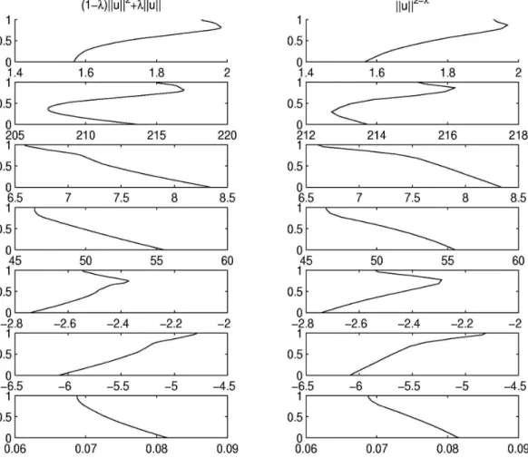
Figure 14 shows the zero path of the homotopy H for those criteria (Tmax =

10N ):

Figure 14: Zero path for the two criteria : λ vs. shooting unknown

As shown in figure 14, there is not much difference between the two criteria in terms of zero path. In fact the zero paths are always quite regular except for one (exceptionally two) ’turn’. However after several numerical experiments, it finally appears that the power criterion is more efficient.

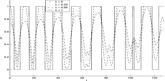
It is quite interesting to visualize the evolution of the norm of the thrust with respect to the homotopic parameter λ along the zero path (figure 15), as it illustrates the evolution from a continuous control (energy problem) to a discontinuous control (mass problem). We can see that this evolution is quite regular, as the energy control already shows some peaks which correspond to the mass control thrust arcs.

Figure 15: Norm of thrust vs. time for several λ and power criterion and Tmax= 10N

Note: for the convex criterion, the evolution of the norm of thrust is similar.

An important point is that this method allows us to discover the control structure without any a priori assumption.

We previously made two hypotheses on the switching function and the adjoint state.

(H1) • first, we assume that Bt_{(x(t))p(t) is non-zero for all t ∈ [t} 0, tf]

(H2) • then, we assume there is no singular arc, that is to say that ψ is never zero on a whole interval.

Figure 16 shows that these assumptions are actually numerically verified:

Figure 16: Norm of thrust, switching function and primer vector vs. time for Tmax= 10N

We can see that Bt_{p is never zero and that the switching function (ψ) has}

only pinpoint zero, on which the control norm switches between 0 and 1. Then we can conclude that our two assumptions (H1) and (H2) are justified.

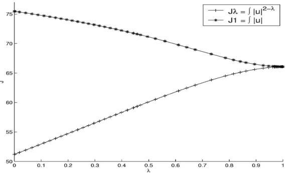
An interesting question is the evaluation of the objective along the zero path. We consider the homotopic objective Rtf

0 ku(t)k

2−λ_{dt. Since kuk ≤ 1,}

this is a lower bound of the mass objectiveRtf

0 ku(t)kdt. Let us see the evolution

of these two objectives (figure 17): Figure 17 shows the evolution of these objectives.

Figure 17: Cost function and L1-norm of optimal control vs. λ

Figure 17 shows us that for λ sufficiently close to 1, the homotopic cost function and the payload cost are really close, which gives a precise minimiza-tion of our mass objective. This property could be used as a numerical stop criterion for convergence of the algorithm. Instead of trying to reach λ = 1, one could stop when the two costs are close enough, which would indicate that we are not far from the best true cost anyway.

Initialization problem : another homotopy

Addressing lower thrust transfers, while decreasing the maximum norm of thrust, we encountered some difficulties with the initialization. In fact, ini-tialization consists of solving the energy problem (λ = 0). With the single shooting method we use, this energy problem itself becomes hard to solve di-rectly when the thrust is below 5 Newtons (we consider a vehicle of initial mass 1500 kg.).

In order to solve this initialization problem, we introduce another homo-topy, which is based on the fact that when the initial and final conditions are the same, the identically null control is a trivial and unique solution. To apply this idea, we introduce the homotopic parameter λ in the initial conditions of our energy problem as follows:

(PICλ )                        minRtf t0 ku(t)k 2_dt

dynamics of state and costate unchanged Pλ(t0) = (1 − λ)P (tf) + λP (t0)

exλ(t0) = (1 − λ)ex(tf) + λex(t0)

eyλ(t0) = (1 − λ)ey(tf) + λey(t0)

hxλ(t0) = (1 − λ)hx(tf) + λhx(t0)

hyλ(t0) = (1 − λ)hy(tf) + λhy(t0)

Other conditions unchanged

It can easily be demonstrated that the shooting function S0

IC(z) associated

with problem (P0

IC) accepts z = (0, 0, 0, 0, 0, 0, 0) as the unique zero. With a

discrete continuation it is possible to find a zero of S1

IC(z), which allows us

to initialize our main homotopy. With this method we were able to find an initialization for a thrust of 0.1 Newton. An interesting aspect of this method is that it requires no preliminary knowledge concerning the solution, such as a solution for a greater thrust for instance.

Global solution search

By using the homotopy on initial conditions and then the main homotopy with the power criterion, we managed to solve our mass problem for thrust down to 0.1 Newton. But looking at the evolution of the final mass with respect to the final time (figure 18) , we can see an annoying phenomenon:

Figure 18: Final mass (kg) vs. final time multiplier for Tmax = 10N

In this figure we can see that the final mass we find is not monotonic with respect to the final time. However it should be because any solution for a given tf also holds for a greater transfer time, by completing it with null thrust after

tf (intuitively the more time we have to do the transfer, the more fuel we can

save). We can then conclude that our solving led us to local solutions. The most annoying is that some of those local solutions are really bad in terms of final mass : we can lose more than 30 kg on a total consumption of less than

150 kg.

Those local solutions are probably due to the fact that Lf is free. Then

our aim will be to search the optimal Lf (Loptf ) which will give us the optimal

number of revolutions and the optimal rendez-vous on the final orbit. We will achieve that purpose by solving the problem for a various number of fixed Lf.

Note: Once we have Lopt_f we will be able to solve rendez-vous problem by setting Lf according to the rendez-vous and to Lopt_f .

But first, this implies a little change on our boundary conditions and more precisely we have this transformation :

pL(tf) = 0 becomes L(tf) = Lf

To set this final longitude (Lf) we use the same approach as for the final

time tf. We first solve the minimum longitude problem, this resolution gives

us a Lfmin on which a multiplier cLf is applied:

Lf = L0+ cLf(Lfmin− L0)

Of course, cLf must be strictly greater than 1 if we want the transfer to be

feasible.

The minimum time and the minimum longitude problems are very close, and just as we had the empiric relation (R0), we found that the following relation numerically holds:

(Lfmin − L0)T max ≈ C (R1)

With our problem constants we have:

Lfref = L0+

Lfmin− L0

TM ax

≈ 267.54 rad

Note that here, Lfref_2π−L0 is the minimum number of revolutions for a thrust of 1 Newton.

From now on, the problem we want to solve is defined by two multipliers ctf and cLf and by the maximum thrust Tmax. This problem is not too far from

the previous one, the main difference is that the homotopy on initial conditions does not accept 0 as a solution for λ = 0. Yet it is still easy to compute a solution of (Pλ

IC) with our single shooting method. Now let us examine the

impact of the choice of the final longitude multiplier cLf. For a given ctf, if we

solve the problem for a range of cLf and then plot the final mass with respect

Figure 19: mf (kg) vs. cLf for Tmax = 10N and various ctf

In this figure, we can see that there is a cLf that maximizes the final mass

for a given ctf and Tmax, we call it cLfopt(ctf, Tmax). It is important to note

that in the neighbourhood of this cLfopt(ctf, Tmax) all cLf remain quite good

in terms of final mass, and that this neighbourhood is larger when ctf grows

(and also when Tmax decreases). This implies that the loss of weight due to a

rendez-vous will not be significant. Of course it would be interesting to have an idea of the value of cLfopt, in order to choose a cLf that gives an optimal

final mass. But is there a way to properly approximate this cLfopt(ctf, Tmax)

without having to explore many values of cLf? The answer is yes, as shown by

figure 20:

Figure 20: cLfopt vs. ctf for various Tmax

In this figure we can see that the numerical relation between cLfopt and

ctf is nearly linear. By using the fact that in the neighbourhood of cLfopt the

final mass remains quite good, we can use a linear relation to approximate the cLfopt, which still depends on Tmax. The linear approximation for various is

Tmax (table 2).

Table 2: Linear approximation of cLfopt Tmax (N.) a b 5 1.129 0.083 2.5 1.122 0.092 1 1.123 0.090 0.5 1.117 0.099

We can see that the values of a and b are quite close for the different Tmax, and the variations could be of numerical nature. Therefore, we can

reasonably suspect that the linear dependency linking cLfopt and ctf is actually

independent from the maximum thrust Tmax. Yet, the mathematical origin of

this possible relation is still an open question.

Interpretations

First, figure 21 shows the evolution of state, costate and control with respect to time:

Figure 21: State, costate, control vs, time for Tmax = 10N , tf = 1.5tmin

first column: state (P, ex, ey, hx, hy, L, m), second column: costate

(pp, pex, pey, phx, phy, pL, pm), third column: control (q, s, w, ||u||)

• The parameter P (first row and column) is before the last correction a little bit superior to the target value, and this is the only exception to its monotony.

• The eccentricity vector (ex, ey) (second and third row, first column)

de-creases in its first component ex and oscillates (negative on perigee and

positive on apogee) in its second component ey which is nearly negligible

with respect to ex. Note that at the end of the transfer the eccentricity

is nearly zero and then the orbit is nearly circular.

• The inclination vector (hx, hy) (fourth and fifth row, first column)

de-creases in norm regularly to zero. And the component hy also shows

some oscillations.

• The longitude L (sixth row and first column) is expressed on [−1; 1] (L = L modulo 2π

π − 1). Due to the fact that ey is nearly negligible with

respect to ex, when L goes smoothly through zero it is approximatively

the apogee and when L goes abruptly through zero it is approximatively the perigee.

• The costate of the mass m (last row, second column) decreases regularly to zero, thus satisfying the final constraints.

• Most of the thrust is transverse.

Figure 22 shows the trajectory associated with figure 21:

Figure 22: Optimal trajectory for Tmax = 10N and ctf = 1.5

Note : figure of steepness (last one) is scaled for better visibility

In the figure 22, one can see that most of burn maneuvers are performed around the apogees. This can easily be explained by the fact that apogee is

the best place for an orbit-raising maneuver and a plane change as the speed of the satellite is smaller that everywhere. The final perigee maneuvers seem to be here for correcting small errors in the apogee.

It is quite obvious that in this thrust strategy, there are no thrust arcs at perigee, except for the last perigees which are not really perigee as the eccentricity is nearly zero. It is important to note that this is the visible difference between ’global’ and local solutions (in a local solution, there are some thrust arcs around first perigees).

If we increase ctf (and then tf) we always have this type of thrust strategy

with more revolutions: there are more thrust arcs that are shorter.

Another interesting remark is that the increase of the final mass with re-spect to tf is less and less important but always strictly positive as far as we

pursued our experiments. This can give some hints regarding the existence of a solution to our problem with free final time, the question being: is there a reach limit or an asymptote.

Figure 23 shows the final mass with respect to ctf for various Tmax:

Figure 23: mf vs. ctf for various Tmax

This figure is very interesting because we can see that, for a given ctf, the

final mass is nearly independent of Tmax. This could eventually give a criterion

for the validity of a solution. We note that this independence is also true in the limiting case of an impulsive transfer where the consumption only depends on the change in the semimajor axis and inclination of the transfer. However in our case the consumption also depends on the fixed final time.

Another interesting application of this empiric law is that if we want a specific payload, we can deduce the corresponding transfer time coefficient, and thus the transfer time at the given thrust.

Low thrust results

Figure 24 shows a trajectory for a thrust of 0.1N :

Figure 24: Trajectory for Tmax = 0.1N. and tf = 1.5tmin

With the optimal strategy we have approximatively 2 switchings per revo-lution (if we do not count the thrusts arcs on the last perigees). The number of revolutions for a given tf is nearly inversely proportional to Tmax. That

is why we have (for ctf = 1.5) 7.5 revolutions at 10 N and approximatively

750 revolutions at 0.1 N. That implies more than 1500 switchings and leads to some difficulties in computing the shooting function with precision.

With the PC method we were able to find the solution of the problem with a thrust of 0.1 N in reasonable time. Table 3 shows some results:

Table 3: Execution time for various Tmax, on a SUN-Blade 1000

Tmax ctf Nb. of Nb. of Execution Execution

revolutions switch time (IC)a _{(s.) time (PC)}b _(s.)

10 1.5 7.5 18 3.6 90 5 1.5 15 36 7.1 115 2.5 1.5 30 73 15.9 281 1 1.5 74.5 179 37.9 2121 0.5 1.5 149 360 48.5 698 0.2 1.5 377 915 126.4 13759 0.1 1.5 754 1786 1425 28185

a: execution time for initial condition homotopy b: execution time for energy to minimum fuel homotopy

Note: problem resolution at 0.1N is quite difficult, yet even lower thrusts would lead to prohibitive transfer time (several years)

Conclusion

Thus, it appears that the homotopic approach combined with the single shoot-ing method is a good choice for an orbital transfer with maximization of the final mass at low thrusts. A particularly important point is that we did not have to make any assumptions about the number of switches of the control, which is often the case (typically with the multiple shooting method). Be-sides, we managed to solve this problem with a reasonable execution time for really low thrusts (0.1 Newton), which involve several hundred thrust arcs for a transfer time of several months. Moreover, the resolution at these low thrusts revealed a strong structural regularity of the optimal control, with thrust arcs located at the apogees and last perigees. This seems to be coherent with the physics of the orbital transfer, and once again was obtained without any a pri-ori informations concerning the physical problem. We also found interesting results regarding the evolution of the final mass with respect to the final time, with several empiric laws of practical interest, probably linked to this regular-ity, as well as the apparent independence of the final mass with respect to the maximal thrust. This might shed some light on the possible non-existence of a solution with free final time, which is still an open question. Some future de-velopments we are currently working on include the study of a non autonomous formulation of the problem, with longitude instead of time as the integration variable, and some additional constraints, such as cone constraint on thrust direction, or state constraints (eclipses). One important question for these problems is whether the prerequisites of predictor-corrector (PC) methods are met or not. In the latter case, the slower simplicial methods have to be used instead of the predictor-corrector continuation.

Acknowledgments

This research was supported by the French Ministry of Superior Education and Research, the CNRS and the French Space Agency1_.

We also wish to thank the reviewers very much for their work and useful comments on this paper, especially the enlightening qualitative remarks on the results.

References

[1] L.C.W. Dixon and Z.A. Maany: To Bus and back, Proceedings of the Sec-ond International Symposium on Spacecraft Flight Dynamics, Darmstadt, FR Germany, 20-23 October 1986 (ESA SP-255, Dec 1986).

[2] M.C. Bartholomew-Biggs, L.C.W. Dixon, S.E. Hersom, Z.A. Maany: The solution of some difficult problems in low-thrust interplanetary trajectory optimization, Optimal Control Applications and Methods, Vol 9, 229-251, 1988.

[3] H.J. Oberle and K. Taubert: Existence and Multiple Solutions of the Minimum-Fuel Orbit Transfer Problem, Journal of Optimization theory and applications, Vol.95 No.2 pp.243-262, November 1997.

[4] S. Geffroy and R. Epenoy: Optimal Low-thrust transfers with constraints - Generalization of averaging techniques, Acta Astronautica Vol 41, No 3, pp 133-149, 1997.

[5] JB.Caillau, J.Gergaud, T.Haberkorn, P.Martinon and J.Noailles: Numer-ical optimal control and orbital transfers, Workshop Optimal Control, Greifswald, October 2002.

[6] J.B. Caillau and J. Noailles: Coplanar control of a satellite around the earth, ESAIM: Control, Optimisation and Calculus of Variations, February 2001, Vol. 6, pp. 239-258

(http://www.edpsciences.org/articles/cocv/abs/2001/01/cocvVol6-9/cocvVol6-9.html)

[7] T.C Le and J. Noailles: Contrˆole optimal et transfert orbital `a tr`es faibles pouss´ees, Equations aux D´eriv´ees Partielles, pp 705-725, Gauthier-Villars, 1998.

[8] J.B. Caillau, J. Gergaud and J. Noailles: TfMin: Short Reference Manual, Optimization Online Digest 2002/07/511, 2002

(http://www.optimization-online.org/DB HTML/2002/07/511.html)

[9] E.Allgower, K.Georg: Numerical continuation methods. An introduction, Springer-Verlag, 1990.

[10] E.Allgower, K.Georg: Numerical path following In P. G. Ciarlet and J. L. Lions, editors, Handbook of Numerical Analysis, volume 5, North-Holland (1997) 3-207.

(http://www.math.colostate.edu/emeriti/georg/georg.publications.html)

[11] E.Allgower, K.Georg: Piecewise Linear Methods for Nonlinear Equations and Optimization, Journal of Computational and Applied Mathematics, volume 124, Special Issue on Numerical Analysis 2000: Vol. IV: Optimiza-tion and Nonlinear EquaOptimiza-tions, 2000.

(http://www.math.colostate.edu/emeriti/georg/georg.publications.html)

[12] C.B. Garcia and W.I. Zangwill: An approach to homotopy and degree theory, Mathematics of operations research Vol.4 No.4, 1979.

[13] L.T. Watson: HOMPACK90: A Suite of Fortran 90 Codes for Globally Convergent Homotopy Algorithms, Netlib

[14] T. Haberkorn, J. Gergaud and J. Noailles: MfMax: Short Reference Man-ual.

(http://www.enseeiht.fr/apo/mfmax/index.html)

[15] L.T. Watson: Fixed points of C2 _{maps, Journal of Computational and}

Applied Mathematics, Vol.5, No.2, 1979, pp. 131-139.

[16] L.T. Watson: A Globally Convergent Algorithm for Computing Fixed Points of C2 _{Maps, Applied mathematics and computation, Vol.5, 1979,}

pp.297-311.

[17] L.T. Watson: An algorithm that is globally convergent with probability one for a class of nonlinear two-point boundary value problems, Society for Industrial and Applied Mathematics, Vol.16, No.3, June 1979, pp.394-401.

[18] P.Martinon, J .Gergaud and J.Noailles: Simplicial homotopy: an applica-tion to orbital transfer, Technical report (code descripapplica-tion and user guide) RT/APO/02/3, ENSEEIHT-IRIT, June 2002