HAL Id: hal-00329339
https://hal.archives-ouvertes.fr/hal-00329339
Submitted on 14 Jul 2004
HAL is a multi-disciplinary open access
archive for the deposit and dissemination of
sci-entific research documents, whether they are
pub-lished or not. The documents may come from
teaching and research institutions in France or
abroad, or from public or private research centers.
L’archive ouverte pluridisciplinaire HAL, est
destinée au dépôt et à la diffusion de documents
scientifiques de niveau recherche, publiés ou non,
émanant des établissements d’enseignement et de
recherche français ou étrangers, des laboratoires
publics ou privés.
and cusp: Cluster EDI observations
H. Vaith, G. Paschmann, J. M. Quinn, M. Förster, E. Georgescu, S. E.
Haaland, B. Klecker, C. A. Kletzing, P. A. Puhl-Quinn, H. Rème, et al.
To cite this version:
H. Vaith, G. Paschmann, J. M. Quinn, M. Förster, E. Georgescu, et al.. Plasma convection across
the polar cap, plasma mantle and cusp: Cluster EDI observations. Annales Geophysicae, European
Geosciences Union, 2004, 22 (7), pp.2451-2461. �hal-00329339�
Geophysicae
Plasma convection across the polar cap, plasma mantle and cusp:
Cluster EDI observations
H. Vaith1, G. Paschmann1, J. M. Quinn2, M. F¨orster1, E. Georgescu1, S. E. Haaland1, B. Klecker1, C. A. Kletzing3, P. A. Puhl-Quinn1,2, H. R`eme4, and R. B. Torbert2
1Max-Planck-Institut f¨ur extraterrestrische Physik, 85748 Garching, Germany 2University of New Hampshire, Durham, NH 03824, USA
3University of Iowa, Iowa City, IA 52242, USA 4CESR-CNRS, 31028 Toulouse, France
Received: 2 October 2003 – Revised: 16 March 2004 – Accepted: 14 April 2004 – Published: 14 July 2004 Part of Special Issue “Spatio-temporal analysis and multipoint measurements in space”
Abstract. In this paper we report measurements of the
po-lar cap convection obtained with the Electron Drift Instru-ment (EDI) on Cluster. We use 20 passes that cross the polar cap between its dayside and nightside boundaries (or vice versa) at geocentric distances ranging from about 5 to about 13 RE, and at interspacecraft separations (transverse
to the ambient magnetic field) between a few km and almost 10 000 km. We first illustrate the nature of the data by pre-senting four passes in detail. They demonstrate that the sense of convection (anti-sunward vs. sunward) essentially agrees with the expectations based on magnetic reconnection oc-curring on the dayside or poleward of the cusp. The most striking feature in the EDI data is the occurrence of large-amplitude fluctuations that are superimposed on the average velocities. One type of fluctuation appears to grow when ap-proaching the dayside polar cap boundary. The examples also show that there is a variable degree of inter-spacecraft correlation, ranging from excellent to poor. We then present statistical results on all 20 passes. Plotting 10-min averages of the convection velocities vs. IMF Bzone recovers the
ex-pected dependence, albeit with large scatter. Looking at the variances computed over the same 10-min intervals, one con-firms that there is indeed one type of contribution that grows towards the dayside boundary, but that variances can be high anywhere. Finally, computing the inter-spacecraft correla-tions as a function of their separation distance transverse to the magnetic field shows that the average correlation drops with increasing distance, but that even at distances as large as 5000 km the correlation can be very good. To put those scales into context, the separation distances have also been scaled to ionospheric altitudes where they range between a few hundred meters and 600 km.
Correspondence to: H. Vaith
Key words. Magnetospheric physics (plasma convection;
instruments and techniques; magnetopause, cusp and bound-ary layers)
1 Introduction
Magnetospheric convection is primarily driven by magnetic reconnection. For southward IMF, reconnection occurs along an X-line on the dayside magnetopause. Once intercon-nected, open magnetic flux tubes are carried by the solar wind over the poles downstream, penetrating deeper and deeper into the magnetotail (where they eventually will re-connect again): anti-sunward convection of magnetic flux over the polar caps is the result. The solar wind plasma mov-ing along these field lines fills a region, the plasma mantle , that is ever widening as a result of the superposition of field-aligned motion and inward convection.
For northward IMF, reconnection can occur poleward of the cusps, between interplanetary magnetic field lines and open tail-lobe field lines (see Lockwood and Moen, 1999, and references therein). Those lobe field lines then move toward the X-line located behind the cusps. After reconnec-tion, one segment of these lobe field lines is disconnected from the Earth and stripped off the top of the tail lobe, while the other segment is pulled to the flanks of the magneto-sphere. The result is a circulation pattern, often described as tail lobe stirring, with sunward convection (over part of the polar cap) as a necessary consequence of reconnection under northward IMF. Details of the pattern depend on IMF
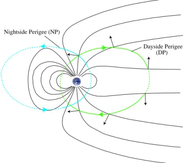
Dayside Perigee (DP) Nightside Perigee (NP)
Fig. 1. The two types of orbits selected for this study, denoted Nightside Perigee (NP) and Dayside Perigee (DP), respectively. The solid parts denote the portions over the polar cap and into the polar cusps. The black arrows show the orientation of the ˆes-axis used to define the sense of the convection in the GSE (X, Z)-plane.
Much of our knowledge of flow in the polar cap comes from ground observations with radars and magnetometers. They provide almost synoptic maps, but have limited spatial and temporal resolution. The SuperDARN radars, for ex-ample, perform a scan over 16 discrete directions every two minutes and use range gates of approximately 45 km along the line of sight. Preprocessing of the data yields a spatial resolution of approximately 100 km (Ruohoniemi and Baker, 1998). Convection measurements from low-altitude space-craft have contributed much as well. They traverse the po-lar cap in about 15 min every 90 min. By contrast, Cluster crosses the polar cap magnetic field lines at geocentric dis-tances of 5–13 RE(see Fig. 1), where the polar cap is much
larger as a result of the divergence of the magnetic field. Cou-pled with the small orbital velocity at these altitudes, a polar cap traversal takes typically 4 h or longer. Solar wind condi-tions are rarely stable enough over such long times to infer, say, the polar cap potential from integration along the orbit. But, by the same token, the residence times over the polar cap are long enough to allow observations of the response to IMF changes.
The expansion of the flux tube diameters and the slow or-bital motion also means that even moderate time resolution measurements translate into excellent spatial resolution when mapped into the ionosphere. Over the central polar cap the Cluster spacecraft speed is 3–4 km s−1. Even a 1 s-resolution measurement (as provided by EDI) at 100 nT maps to only a few hundred meters in the ionosphere. Similarly, Cluster spacecraft separations of 100 to 10 000 km map to very small scales in the ionosphere.
The purpose of the present paper is to report convec-tion measurements made with the Electron Drift Instrument (EDI) over the polar cap between its dayside and nightside boundaries. Emphasis is on the dependence on the IMF ori-entation, the characterization of rapid temporal variations, and the correlation between the Cluster spacecraft. In Sect. 2 we briefly discuss the EDI technique and data analysis meth-ods. Section 3 presents four polar cap passes that illustrate the nature of the observations. In Sect. 3.3 statistical results on the average convection, their fluctuations and the inter-spacecraft correlations are presented for a total of 20 passes. The results are discussed and summarized in Sect. 4.
2 Instrumentation and data analysis
The Electron Drift Instrument (EDI) measures the plasma convection velocity through the injection of artificial elec-tron beams. The EDI technique, hardware, operation, and data analysis method have been described in detail in ear-lier publications (Paschmann et al., 1997; Quinn et al., 2001; Paschmann et al., 2001). Briefly, the technique is based on the injection of two electron beams at right angles to the am-bient magnetic field, and the search of the two directions (within the B⊥-plane) that return the beams to their
asso-ciated detectors after one or more gyrations. Knowledge of the positions of the guns and of the firing directions uniquely determines the drift velocity. This is the basis of the trian-gulation technique. Through triantrian-gulation one directly de-termines the “drift-step” vector d, which is the displacement of the electrons after a gyro time Tg. The location in the
B⊥-plane, from which electrons reach the detector after one
gyration, can be viewed as the “target” for the electron beam. Our standard analysis technique consists in selecting all returning beams within a certain time-interval, typically one spacecraft spin, i.e. approximately 4 s (but often also 1/2 or 1/4 spin), and to perform an automated determination of the drift velocity. The triangulation analysis determines the drift step by searching for the target-point that minimizes an appropriate “cost-function”. For each grid-point in the
B⊥-plane, the cost-function is constructed by adding up the
(squared) angle-deviations of all beams in a chosen time in-terval from the direction to that grid-point, normalized by the (squared) error in the firing directions. The grid-point with the smallest value of the cost-function is taken as the target. Errors in magnitude and direction are obtained from the (re-duced) chi-square surface.
When the drift step becomes large, the triangulation method degenerates. Under these conditions, however, the times-of-flight of the electrons in the two beams become measurably different and can be used to determine the drift step (ToF-method). The measured times-of-flight are also used to identify the number of gyrations the emitted electrons perform prior to their detection. This information is essential for calculating the drift velocity from either the triangulation or the time-of-flight technique.
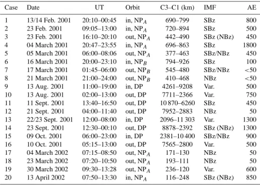
Table 1. Key characteristics of the investigated cases.
Case Date UT Orbit C3–C1 (km) IMF AE
1 13/14 Feb. 2001 20:10–00:45 in, NPA 690–799 SBz 800 2 23 Feb. 2001 09:05–13:00 in, NPA 720–894 SBz 500 3 23 Feb. 2001 16:10–20:10 out, NPA 442–490 SBz (NBz) 450 4 04 March 2001 20:47–23:55 in, NPA 696–863 SBz 1800 5 05 March 2001 06:00–08:06 out, NPA 377–463 SBz/NBz 450 6 16 March 2001 20:00–23:10 in, NPB 794–926 SBz 100 7 17 March 2001 01:45–06:00 out, NPB 545–480 SBz/NBz <50 8 21 March 2001 21:00–24:00 out, NPB 410–468 NBz <50 9 13 Aug. 2001 11:00–19:00 in, DP 4261–9208 Var. 500 10 13 Aug. 2001 02:00–13:00 out, DP 7711–2366 Var. 750 11 11 Sept. 2001 13:40–16:50 out, DP 10 870–6260 SBz 450 12 21 Sept. 2001 04:00–11:40 out, DP 7952–2883 NBz 50 13 22/23 Sept. 2001 12:00–08:00 in, DP 2096–11 303 Var. 1300 14 23 Sept. 2001 12:30–00:10 out, DP 8878–2392 SBz (NBz) 1300 15 09 Oct. 2001 06:00–23:00 in, DP 2381–10 400 SBz/NBz 900 16 10 Oct. 2001 05:15–13:00 out, DP 7565–2800 Var. 500 17 04 March 2002 07:15–08:50 out, NPA 171–130 NBz 50 18 23 March 2002 07:20–10:50 out, NPA 193–111 NBz 50 19 30 March 2002 09:30–13:28 out, NPA 236–120 Var. 600 20 13 April 2002 07:50–13:30 in, NPA 116–248 SBz (NBz) 850
To calculate the drift velocity from the times-of-flight, the beam firing directions need to be separated into two classes, one comprising beams that have a component parallel to the target direction; the other class consists of beams with anti-parallel components. The target direction is not known a priori, but found (with an ambiguity of 180◦ ) by vary-ing a reference direction such that the standard deviations of the distributions of beam firing directions in the two classes with components parallel and anti-parallel to the reference direction around their respective average directions are min-imized. The ambiguity in the target direction is removed by calculating the average time-of-flight for each of the two classes. The class of beams with the larger average times-of-flight then constitutes the beams directed towards the target (because those execute slightly more than one gyration), the other class constitute those directed away from the target (ex-ecuting slightly less than one gyration). If the magnetic field had constant magnitude during the analysis interval (e.g. a spin period), then the drift magnitude (and its errors) could simply be computed from the difference between the aver-age magnitude (and standard deviation) of the times-of-flight of the towards and away beams. But as this assumption is often not fulfilled, we use the high-resolution magnetic field data from the FGM instrument (Balogh et al., 1997), together with the best available calibration parameters, to compute the gyro time and its variation during the analysis interval. For each beam we then take the differences between the mea-sured times-of-flight and the value of the gyro time at the time the beam was recorded. These differences are then summed separately for the towards and away sets, and the
drift velocity (and its error) are computed from the difference between the two averages. The multi-gyration assignment is based on a comparison between the measured times-of-flight and the gyro-time. We use the gyro-times based on the high-resolution FGM data for this purpose as well.
Convection velocities can also be derived from the EFW double probe electric field measurements (Gustafsson et al., 1997) and from the ion bulk velocities measured by the CIS instrument (R`eme et al., 2001). By their very nature, the EDI measurements offer some unique advantages over these techniques, but also suffer from a number of limitations. The advantages over the double-probe technique lie in EDI’s in-sensitivity to spacecraft-induced wake effects which can ob-scure the small electric fields found, for example, in the low-density environment over the polar caps. Moreover, EDI measures both components of the convection velocity for all orientations of the magnetic field, while the double-probe technique, unless when using a boom along the spin axis of the spacecraft, measures only the component of the elec-tric field in the spin plane. The drift velocities computed as the perpendicular component of the CIS bulk velocities nat-urally suffer from poor counting statistics when densities are low. Bulk velocities are also affected by pressure gradients to which EDI is immune. On the other hand, EDI is adversely affected in three ways. First, rapid time variations (on spin-period scale) in magnetic and/or electric fields can cause vari-ations in the drift velocity (magnitude and direction) that are too rapid to be tracked by the electron beam pointing hard-and software. Second, magnetic field magnitudes which are too low make the gyro radius of the emitted electrons so large
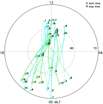
Fig. 2. Projection of the 20 passes into the polar ionosphere along the Tsyganenko-2001 model magnetic field. Solid and dashed lines are for orbits in the Northern and Southern Hemispheres, respec-tively. Nightside Perigee orbits (NP) are shown in blue, Dayside Perigee orbits (DP) in green, as in Fig. 1.
that the angular divergence of the beams makes the return-ing flux density too low to be detected. Third, the pres-ence of ambient electrons at the beam energy cause back-ground counts that can reduce the signal-to-noise ratio until the beams are no longer recognized.
Given the advantages and shortcomings of EDI, it is evi-dent that the polar cap is an ideal environment for EDI be-cause the three adverse effects just mentioned are essentially absent and the other techniques quickly reach their limita-tions, as demonstrated in a separate publication (Eriksson et al., submitted to Ann. Geophys., 20031).
To put the EDI data into the proper context, we use the plasma densities and bulk velocities from the CIS-HIA in-strument and the magnetic field magnitude measured by the FGM instrument.
3 Observations
3.1 Data selection
To characterize the convection observed with EDI over the polar cap and its dayside boundary regions (cusp and plasma mantle), we have selected a total of 20 crossings. In order to have coverage of polar cap, plasma mantle and cusp we have chosen orbits that have their plane close to the noon-midnight 1Eriksson, A. I., et al.: Electric Field Measurements on
Clus-ter: Comparing the Double-Probe and Electron Drift Techniques, submitted to Ann. Geophys., 2003.
meridional plane. A further criterion for the selection of the orbits was the requirement to have continuous coverage with EDI data. Key characteristics of the selected orbits are pro-vided in Table 1. These include the UT intervals, the sepa-ration distance between C1 and C3, an indication of the IMF orientation, and the maximum AE index during the crossing. The selected orbits are categorized into two types, as il-lustrated in Fig. 1. “Nightside Perigee” orbits (NP) cross the nightside auroral oval into the polar cap and traverse the po-lar cap until they encounter the cusp or exit into the mag-netosheath. “Dayside Perigee” orbits (DP) cross the north-ern cusp at mid-altitudes and then spend a long time in the tail lobes before entering the plasma sheet near apogee. DP-orbits never cross the magnetopause. (The above description applies to outbound passes, i.e. Northern Hemisphere. The sequence is reversed for inbound passes.)
As the figure shows, the two orbit types sample the dayside and nightside boundaries of the polar cap at very different altitudes. Only near the central polar cap are they at the same altitude. Of the 20 selected passes, 12 are of type NP, 8 of type DP.
NP-orbits can conveniently be subdivided into those orbits (NPA) that exit the polar cap directly from the lobes, i.e.
pole-ward of the cusp or via the distant (exterior) cusp, and those (NPB) that cross the distant cusp, but then enter the dayside
magnetosphere before crossing the (dayside) magnetopause into the magnetosheath. Of the 12 NP passes, 9 are of type NPAand 3 of type NPB.
Figure 2 shows the 20 passes, mapped into the ionosphere along a model magnetic field (Tsyganenko, 2002). The num-bers in Fig. 2 refer to the case numnum-bers in the table.
The limitations inherent in the EDI technique noted in Sect. 2 affect the different types of passes in different ways. NP passes can suffer from a B which is too low, being encountered before the magnetopause or within the distant cusp. As a consequence, the data sometimes stop before the cusp crossing was completed or the magnetopause was reached. DP passes exit the polar cap when the spacecraft enter the plasma sheet at large distances where B is also of-ten too low.
3.2 Case studies
In this section we will discuss four cases in some detail, in order to illustrate the character of the data. The con-vection velocities are presented in a coordinate system that takes into account the large change in magnetic field incli-nation encountered along the Cluster orbit (cf. Fig. 1) and the fact that, by its very nature, the convection velocity, V , is a two-dimensional vector in the plane perpendicular to B. The axes of this coordinate system are ˆes and ˆed, defined
as ˆes=B× ˆyGSE/|B× ˆyGSE|and ˆed=ˆes×B/B, respectively,
and we denote the components along them as Vs and Vd.
With this definition the unit vectors ˆes, B/B and ˆed
con-stitute a right-hand coordinate system and a positive Vs
al-ways maps to sunward convection in the ionosphere, even if the GSE-x component of the convection velocity becomes
Fig. 3. Measured time-series for an inbound pass of Cluster-3 over the southern polar cap on 13 February 2001. The top two panels show the convection velocities after applying a 30 s-smoothing to the full-resolution EDI data; Vs is the component along the ˆes-axis introduced in the text, Vdthe component along ˆed. The 3rd and 4th panels show the ion density, N, and the parallel component of the bulk velocity, Vk,
measured by CIS-HIA, the 5th panel the magnetic field strength measured by FGM. Universal time, and GSE positions are shown along the bottom of the latter panel. The bottom panel finally shows the IMF clock-angle derived from the ACE magnetic field measurements, shifted for the propagation delay. Values of 0◦and 180◦denote fields that when projected into the GSM (Y, Z)-plane are pointing due north and due south, respectively.
negative where the GSE-z component of B switches sign in the magnetotail (cf. Fig. 1). The unit vector ˆedalways has a
positive GSE-y (i.e. duskward) component. In fact, for the passes selected for this study the angle between ˆedand ˆyGSE
is on average only 16 degrees and the component of the con-vection velocity V along ˆedis thus in most cases very similar
to the GSE-y component of V .
3.2.1 13 February 2001
The first case, shown in Fig. 3, is an inbound pass of type NPA that begins in the magnetosheath, encounters a low-B
interval that marks the magnetopause, before entering the southern tail-lobe near 20:08 UT and heading for perigee on the nightside. The IMF is directed southward throughout the time shown, as can be seen from the IMF clock angle in the bottom panel, which stays within 45◦of 180◦. As this orien-tation favors dayside reconnection, Vs is consistently
nega-tive, corresponding to anti-sunward convection, as expected. At the beginning of the pass the spacecraft position maps to an ionospheric position that, according to convection models (e.g. Weimer, 1996) is located near the dayside portion of the dusk convection cell. This would explain the initially nega-tive Vd component (at this time the angle between the ˆed
-axis and ˆyGSEis approximately five degrees and Vd is thus
very close to the GSE-y component of the convection ve-locity.) Also, as expected for dayside reconnection, plasma at elevated density that is flowing along B away from the Earth extends well into the tail lobe, i.e. the spacecraft has entered the plasma mantle. (Note that the CIS-CODIF in-strument observes upstreaming O+ions over the polar cap on this crossing. This means that the densities shown in Fig. 3, which are calculated from the CIS-HIA measurements un-der the assumption that all ions are protons, are not strictly correct.)
An important feature to note is the large-amplitude fluc-tuations that are superimposed on the average convection velocities. These fluctuations have time scales of approxi-mately two to five minutes and amplitudes that are compa-rable to the average velocities. They die out with elapsed time (or distance) from the magnetopause crossing, or when the plasma density has dropped to background values. To-wards the end of the pass the velocities become very small, only 2 km s−1. If one prefers to think in terms of elec-tric fields rather than drift velocities, one should remember that V =1000 E/B, with E in mVm−1, B in nT, and V in km s−1. The 2 km s−1drift velocity just mentioned, which occurs at about 500 nT, thus corresponds to an electric field of 1 mVm−1.
This pass serves as a key example for the comparison be-tween the EDI convection measurements and those from the EFW electric field and CIS bulk velocity measurements2. 3.2.2 11 September 2001
This is a DP pass 6 months later, when perigee is near local noon and apogee in the magnetotail (Fig. 4). The (outbound) pass begins with a crossing of the northern mid-altitude cusp, as evidenced by the peaks in the C1 and C3 density traces that are accompanied by brief Vk flow pulses that are
di-rected downward, i.e., towards the ionosphere. Consistent with their large separation(≈11 000 km, see see Table 1), the cusp encounters by C1 and C3 are displaced by more than 30 min. The spacecraft then enter the plasma mantle (recog-nized by negative, i.e. outward directed Vk), before entering
the polar cap and heading for apogee in the magnetotail. On this day Cluster data collection stopped at 16:50 UT, well before the nightside polar cap boundary.
The IMF is along +Y initially, then flips to −Y at approx-imately 14:21 UT, before becoming more and more south-ward. The average convection is anti-sunward, with some large-amplitude fluctuations superimposed. For this pass we show EDI data for C1, C2 and C3. During the early part of the pass the spaceraft are in very different regions. As a result the velocities differ between the three spacecraft. Af-ter 15:15 UT, however, the convection becomes steady and very well correlated between the spacecraft, which at this time were more than 6000 km apart. This indicates a transi-tion from a crossing of spatial structures to the encounter of large-scale temporal variations.
A noteworthy feature is the transient, sudden reductions in the convection velocity that occur later on, in particular near 16:20, when the IMF is very steady. Such dropouts are common for crossings with large AE, and are the subject of a separate publication3where it is demonstrated that they are associated with global magnetic field reconfigurations. 3.2.3 23 March 2002
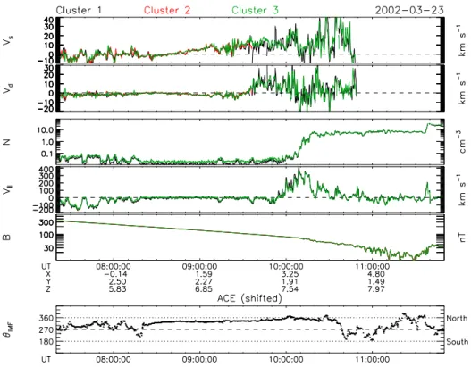
Figure 5 shows an outbound NP pass of the northern po-lar cap, thus showing the reverse sequence of Fig. 3. This time, however, the IMF is directed steadily northward after 08:20 UT. Shortly afterwards Vs becomes positive, i.e. the
convection is now sunward, as expected over the central polar cap for strongly northward IMF (e.g. Reiff and Burch, 1985) for reconnection poleward of the cusp. At about 10:00 UT Cluster enters the cusp, and encounters downward directed plasma jets, with velocities up to 400 km s−1, presumably emanating from the magnetopause equatorward of the recon-nection site. Already when approaching the cusp, and even more so inside, Vs shows large-amplitude fluctuations that
are reasonably well correlated between C1 and C3 (the C2 data stop earlier as a result of operational restrictions).
2in publication by Eriksson, A. I., et al. (see footnote on page 4) 3by Quinn, J. M., et al.: Convection Dropouts in the Polar Cap,
in preparation.
3.2.4 5 March 2001
The final example (Fig. 6) shows an outbound NP pass over the northern polar cap towards the high-latitude magne-topause that is characterized by piecewise stable IMF, start-ing out almost exactly northward, becomstart-ing southward, and then switching back and forth a few more times. On aver-age, the convection direction follows the IMF, but there are very large amplitude waves/fluctuations, commencing with entry into dense upflowing plasma. This case is subject of a separate publication4.
3.3 Statistics
In this section we present some statistical results concerning the dependence of the convection velocity and its fluctuations for all 20 cases listed in Table 1.
3.3.1 Average convection
In this section we look at the average convection as a func-tion of the IMF. Figure 7 shows 10-min averages of convec-tion velocities in the GSE (X, Z)-plane as a funcconvec-tion of IMF
Bz, computed every two minutes for all 20 passes. As
il-lustrated by Fig. 1 the spacecraft altitude varies substantially while passing over the polar cap. As the flux-tube cross sec-tion increases with altitude, so does the convecsec-tion velocity. This explains why the convection velocity shown in Fig. 3, for example, becomes smaller with decreasing distance or in-creasing magnetic field strength. To remove the altitude ef-fect, we do not show in Fig. 7 not the absolute velocities, but instead have scaled them to ionospheric altitudes of approxi-mately 100 km by multiplication with (B/50 000)1/2, where
Bis the ambient magnetic field strength in nT and 50 000 nT is taken as the ionospheric field strength. This scaling ex-plains why the magnitude of the velocities is now of the or-der of 1 km s−1. We denote the scaled convection velocity as
˜ Vs.
The figure shows the expected trend, in spite of the large scatter: for large negative IMF Bz essentially all velocities
are directed anti-sunward ( ˜Vs<0), and the bulk of the
veloc-ities become smaller with increasing IMF Bz. The majority
of the points show negative ˜Vs even for an IMF Bz as large
as +5 nT. Some of the scatter certainly originates from un-certainties in the time-shift applied to the IMF data at times when the IMF orientation changes drastically. More impor-tantly, however, is that reconnection poleward of the cusp does not necessarily imply sunward convection over the en-tire polar cap, because the existence of a cell that is closed within the polar cap implies that both sunward and anti-sunward convection exists (Cowley and Lockwood, 1992). It therefore depends on the spacecraft position which con-vection direction is actually observed. In fact, one of the crossings (21 March 2001, case 8 in Table 1) shows con-sistent anti-sunward convection even though the IMF points 4Puhl-Quinn, P. A., et al.: Cluster measures ULF waves over the
Fig. 4. Data for an outbound pass on 11 September 2001 in the same format as Fig. 3, except that EDI and FGM data are shown for C1, C2, and C3 (using the standard colors black, red and green, respectively), CIS-HIA data for C1 and C3 (not available on C2), and GEOTAIL data are used instead of ACE data for the IMF clock angle.
steadily northward, as the orbit maps to the dawnside of the central cell of the expected convection pattern, where for northward, duskward IMF the sense of convection is indeed anti-sunward.
We have also plotted the same data against the IMF clock-angle. But since no asymmetry with regard to the IMF By
component (i.e. 90◦vs. 270◦clock-angle) was apparent, we do not show it here.
3.3.2 Fluctuations
In Sect. 3.2 we have seen that superimposed on the aver-age convection there are often large-amplitude fluctuations. The level of fluctuations generally appeared to grow when approaching the cusp or magnetopause. To substantiate this finding, we show in Fig. 8 the variances of ˜Vs, computed for
the same 10-min intervals used to construct the data points in Fig. 7, as a function of the GSE-x spacecraft position relative to the position at the time of the closest approach to the cusp or magnetopause. Again, there is large scatter in the data, but the trend for increased variances when approaching the day-side polar cap boundary is apparent in the averages shown by the histogram for distances less than four Earth radii.
A similar though even weaker correlation is seen when plotting the variances vs. the plasma density. This proba-bly simply reflects the fact that the density usually increases when approaching the cusp or magnetopause.
3.3.3 Correlations
In Sect. 3.2 we had noted the variablity of the correlation be-tween the velocities measured by EDI on C1, C2, and C3. To further investigate these correlations we use 60-s averages of the scaled velocities, ˜Vs, to compute the cross-correlation
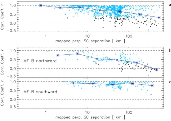
co-efficient between the 3 pairs of spacecraft for 60 min running averages, and plot them against the spacecraft separation dis-tances (projected perpendicular to B). Because of the noted expansion of the flux-tube cross section with altitude, a given spacecraft separation distance implies different scales when occurring at different spacecraft altitudes. To remove this ef-fect, we have used the same scaling factor, (B/50 000)1/2, already used to map the velocities, also for the spacecraft separation distance. The scaling factor ranges approximately from 0.03 to 0.1, and the Cluster separations of a few km up to 10 000 km are consequently mapped to very small scales in the ionosphere, down to a few hundred meters. Even the largest separations correspond to only a few hundred kilome-ters in the ionosphere. The resulting scatter plot is shown in Fig. 9a. It demonstrates that at small separations the corre-lation is almost always very good, while at large distances the correlation varies widely, ranging from very good to very poor.
To determine quantitatively which values for the corre-lation coefficients can be considered significantly different from zero we follow the standard statistical approach. First,
Fig. 5. Data for an outbound pass on 23 March 2002 over the northern polar cap towards the magnetopause, which is crossed near 11:40 UT. The average convection is mostly sunward, consistent with the mostly northward IMF. Note the downward directed high-speed plasma jets observed when entering the cusp near 10:00 UT. There are no useful EDI data after 10:50 UT because of the low and fluctuating magnetic field. EDI data on C2 stop even earlier because of operational restrictions.
Fig. 6. Data for an outbound pass on 5 March 2001 in the same format as previous figures. The pass is characterized by transitions between piecewise stable IMF directions. The convection essentially follows the IMF, on average, but exhibits well correlated fluctuations with very large amplitudes when entering upward flowing plasma (Vk>0). The magnetopause is crossed near 08:10 UT.
Fig. 7. Scaled 10-min averaged convection velocities ˜Vs vs. IMF
Bzfor the 20 cases listed in Table 1. Overplotted in black are the average and standard deviations of the velocities.
Fig. 8. Variances in ˜Vs for the same 10-min intervals as in Fig. 7, as a function of the distance along the GSE x-axis from the dayside polar cap boundary crossing.
we have confirmed that the distributions of the convection ve-locities ˜Vs are very close to Gaussian. Under the additional
assumption (which we want to reject) that the true correlation coefficient is zero, the quantity
t =√ r
1 − r2
√
N −2, (1)
where r is the calculated correlation coefficient and N is the number of points used in the computation of the correlation coefficient, is t distributed (Student’s distribution) with N -2 degrees of freedom. We consider the correlation coeffi-cient to be significantly different from zero if the associated
t-value lies in one of the two tails of the distribution, each of which holds 0.5% of the area of the integrated Student’s distribution function. We have colored the correlation coef-ficients which pass this criterion in Fig. 9a blue. This analy-sis shows that insignificant correlation (colored black) exists mainly for separation distances above 20 km.
tion coefficients into cases of northward and southward IMF, eliminating those 60-min intervals for which the IMF was not steadily pointing northward or southward. In Figs. 9b and c we have plotted the remaining correlation coefficients against the scaled spacecraft separation distance, and we have ap-plied the same criterion as in Fig. 9a, to illustrate the ques-tion of significance of the correlaques-tion coefficients. These scatter plots clearly show that insignificant correlation exists mainly for northward IMF. In fact, for IMF Bz>0 significant
(positive) correlation does not exist for mapped separations larger than approximately 200 km. To quantify the different behaviour for northward and southward IMF we calculate a correlation scale length ξ according to
ξ = P id˜i⊥ri P iri , (2)
where ˜di⊥ are the scaled perpendicular spacecraft
separa-tions and ri are the associated correlation coefficients. The
resulting values of ξ are 31 km and 104 km for northward and southward IMF, respectively.
The smaller correlation scale lengths for northward IMF are consistent with models and observations reported in ear-lier publications. First, when the IMF changes from north-ward to southnorth-ward, open magnetic flux is being added to the polar cap, causing the polar cap to grow until a quasi-steady equilibrium state is reached where the tail reconnection rate, on average, equals the reconnection rate at the dayside mag-netopause (Cowley and Lockwood, 1992). A second con-tributing factor is that there is a tendency for more convection cells for northward IMF (e.g. Reiff and Burch, 1985; Cow-ley and Lockwood, 1992), compared to southward IMF, with more flow reversals along the dawn-dusk line. Furthermore, Maynard et al. (1998) reported the reconnection poleward of the cusp for northward IMF, that leads to lobe cells, to be patchy. Moreover, since the lobe cells for northward IMF are closed within the polar cap, one should, in principle, even be able to observe anticorrelation at larger spacecraft separation distances (if the separation is mainly in the dawn-dusk direc-tion). The trend in Fig. 9b for large separation distances is consistent with this prediction.
4 Summary and conclusions
The findings presented in the previous sections may be sum-marized as follows:
1. On average, the convection velocity shows the expected dependence on IMF-Bz (or clock-angle). However,
there is large scatter, even though the velocities were al-ready averaged over 10 min. While some of the scatter is attributable to uncertainties in the propagation delay of the upstream monitor data, it is also clear that even for stable IMF conditions there are large variations in the 10-min averaged convection velocities that obscure
a
b
c
Fig. 9. (a) Correlation coefficients of 1-h intervals of 60-s smoothed ˜Vsvs. mapped spacecraft separation distances transverse to the magnetic field; correlation coefficients above the significance threshold are colored blue, the others black; (b) and (c) same as (a), except the subset of cases with steady IMF have been separated into IMF northward and southward, respectively. The asterisks interconnected by straight lines show the average trend.
the average behavior. For northward IMF, the convec-tion is not expected to be uniformly sunward over the entire polar cap, but contains regions with anti-sunward convection, the detailed distribution depending on
IMF-By. This effect contributes to the large scatter seen for
northward IMF.
When considering the dependence of in-situ convection measurements one must also not forget that convection is the sum of two intrinsically time-dependent contribu-tions. One is driven by coupling processes at the mag-netopause, primarily by magnetic reconnection, and de-termined by concurrent IMF/SW conditions. The other is driven by tail-processes and related to past history of the IMF/SW and the magnetosphere (Cowley and Lock-wood, 1992). As our cases extend well into the night-side polar cap it is quite likely that some of the varia-tions we observe are due to magnetotail processes. The dropouts noted in conjunction with the 11 September 2001 event (Sect. 3.2.2) are a particularly relevant case at hand.
To make statements about the (co-)existence of the var-ious kinds of convection cells (merging, lobe, viscous) would require one to distinguish the data according to the signs of IMF Byand IMF Bz, as well as the
space-craft position along the dawn-dusk line. This would re-quire more than the limited number of cases available for this study. In particular, we cannot contribute to the
question of the existence of lobe-type cells for south-ward IMF, as they have been reported, e.g. by Burch et al. (1985) and Eriksson et al. (2002).
2. Perhaps the most striking feature in the EDI data is the occurrence of large amplitude fluctuations that are su-perimposed on the average behavior. From inspection of the individual cases, and confirmed by the statisti-cal analysis of all 20 cases, it is evident that there is one type of fluctuation that grow when approaching the cusp/magnetopause boundary and its occurrence is thus not a temporal phenomenon. But there are other cases when large variances seem to occur at random.
One contributing factor to the large fluctuations ob-served in the vicinity of the boundaries, especially the magnetopause, is the motion of the boundaries them-selves. We have cases of multiple magnetopause cross-ings where the sign and magnitude of the EDI velocities match the inward and outward motion of the magne-topause inferred from four spacecraft timing analysis. 3. The unique contribution of Cluster is the ability to
pro-vide multi-point measurements, thus allowing the infer-ence of spatial scales. From correlations of the convec-tion velocities from the three spacecraft where EDI is operative, it appears that the scales, when mapping the spacecraft separation distances down to ionospheric al-titudes, are always larger than 1 km and sometimes, but
data into cases of pure northward and southward IMF shows that the large scales of a few hundred km exist only for southward IMF, whereas for northward IMF poor correlation occurs already at separation distances of only a few tens of km. These results are in qualitative agreement with models and observations reported by Cowley and Lockwood (1992), Reiff and Burch (1985) and Maynard et al. (1998). While it seems hardly sur-prising that scales are larger than 1 km, poor correlation at only a few tens of km separation over the polar cap is surprising and is below the resolution achieved by the SuperDARN radars in their standard scan mode.
Acknowledgement. The authors would like to thank M. Chutter and T. Leistner for data processing support, and the ACE SWEPAM and MAG instrument teams, as well as the GEOTAIL CPI and MGF instrument teams and the CDAWeb for the Solar Wind/IMF data. This work was supported by DLR through grants FKZ:50OC89043 and FKZ:50OC9705, and by NASA through grants NNG04GA46G and NAG5-9960.
Topical Editor T. Pulkkinen thanks S. W. H. Cowley and another referee for their help in evaluating this paper.
References
Balogh, A., Dunlop, M. W., Cowley, S. W. H., Southwood, D. J., Thomlinson, J. G., Glassmeier, K. H., Musmann, G., Luhr, H., Buchert, S., Acuna, M. H., Fairfield, D. H., Slavin, J. A., Riedler, W., Schwingenschuh, K., and Kivelson, M. G.: The Cluster Mag-netic Field Investigation, Space Sci. Rev., 79, 65–91, 1997. Burch, J. L., Reiff, P. H., Menietti, J. D., Winningham, J. D., Heelis,
R. A., Hanson, W. B., Shawhan, S. D., Shelley, E. G., Sugiura, M., and Weimer, D. R.: IMF By-dependent plasma flow and Birkeland currents in the dayside magnetosphere, I. – Dynamics Explorer observations, J. Geophys. Res., 90, 1577–1593, 1985. Cowley, S. W. H. and Lockwood, M.: Excitation and decay of
so-lar wind-driven flows in the magnetosphere-ionosphere system, Ann. Geophys., 10, 103–115, 1992.
Eriksson, S., Bonnell, J. W., Blomberg, L. G., Ergun, R. E., Mark-lund, G. T., and Carlson, C. W.: Lobe cell convection and field-aligned currents poleward of the region 1 current system, J. Geo-phys. Res.-Space, 107(A8), 10.1029/2001JA005041, 2002. Gustafsson, G., Bostrom, R., Holback, B., Holmgren, G., Lundgren,
A., Stasiewicz, K., Ahlen, L., Mozer, F. S., Pankow, D., Harvey, P., Berg, P., Ulrich, R., Pedersen, A., Schmidt, R., Butler, A., Fransen, A. W. C., Klinge, D., Thomsen, M., Falthammar, C.-G., Lindqvist, P.-A., Christenson, S., Holtet, J., Lybekk, B., Sten, T. A., Tanskanen, P., Lappalainen, K., and Wygant, J.: The Elec-tric Field and Wave Experiment for the Cluster Mission, Space Sci. Rev., 79, 137–156, 1997.
Lockwood, M. and Moen, J.: Reconfiguration and closure of lobe flux by reconnection during northward IMF: possible evidence for signatures in cusp/cleft auroral emissions, Ann. Geophys., 17, 996–1011, 1999.
Maynard, N. C., Burke, W. J., Weimer, D. R., Mozer, F. S., Scud-der, J. D., Russell, C. T., Peterson, W. K., and Lepping, R. P.: Polar observations of convection with northward interplanetary magnetic field at dayside high latitudes, J. Geophys. Res., 103, 29–46, 1998.
P., Pagel, U., Bauer, O. H., Haerendel, G., Baumjohann, W., Scopke, N., Torbert, R. B., Briggs, B., Chan, J., Lynch, K., Morey, K., Quinn, J. M., Simpson, D., Young, C., McIlwain, C. E., Fillius, W., Kerr, S. S., Mahieu, R., and Whipple, E. C.: The Electron Drift Instrument for Cluster, Space Sci. Rev., 79, 233–269, 1997.
Paschmann, G., Quinn, J. M., Torbert, R. B., Vaith, H., McIlwain, C. E., Haerendel, G., Bauer, O. H., Bauer, T., Baumjohann, W., Fillius, W., F¨orster, M., Frey, S., Georgescu, E., Kerr, S. S., Klet-zing, C. A., Matsui, H., Puhl-Quinn, P., and Whipple, E. C.: The Electron Drift Instrument on Cluster: overview of first results, Ann. Geophys., 19, 1273–1288, 2001.
Quinn, J. M., Paschmann, G., Torbert, R. B., Vaith, H., McIlwain, C. E., Haerendel, G., Bauer, O., Bauer, T. M., Baumjohann, W., Fillius, W., Foerster, M., Frey, S., Georgescu, E., Kerr, S. S., Kletzing, C. A., Matsui, H., Puhl-Quinn, P. A., and Whipple, E. C.: Cluster EDI convection measurements across the high-latitude plasma sheet boundary at midnight, Ann. Geophys., 19, 1669–1681, 2001.
Reiff, P. H. and Burch, J. L.: IMF B(y)-dependent plasma flow and Birkeland currents in the dayside magnetosphere, II. – A global model for northward and southward IMF, J. Geophys. Res., 90, 1595–1609, 1985.
R`eme, H., Aoustin, C., Bosqued, J. M., Dandouras, J., Lavraud, B., Sauvaud, J. A., Barthe, A., Bouyssou, J., Camus, T., Coeur-Joly, O., Cros, A., Cuvilo, J., Ducay, F., Garbarowitz, Y., Medale, J. L., Penou, E., Perrier, H., Romefort, D., Rouzaud, J., Vallat, C., Alcayd´e, D., Jacquey, C., Mazelle, C., D‘Uston, C., M¨obius, E., Kistler, L. M., Crocker, K., Granoff, M., Mouikis, C., Popecki, M., Vosbury, M., Klecker, B., Hovestadt, D., Kucharek, H., Kuenneth, E., Paschmann, G., Scholer, M., Sckopke (†), N., Sei-denschwang, E., Carlson, C. W., Curtis, D. W., Ingraham, C., Lin, R. P., McFadden, J. P., Parks, G. K., Phan, T., Formisano, V., Amata, E., Bavassano-Cattaneo, M. B., Baldetti, P., Bruno, R., Chionchio, G., di Lellis, A., Marcucci, M. F., Pallocchia, G., Korth, A., Daly, P. W., Graeve, B., Rosenbauer, H., Va-syliunas, V., McCarthy, M., Wilber, M., Eliasson, L., Lundin, R., Olsen, S., Shelley, E. G., Fuselier, S., Ghielmetti, A. G., Lennartsson, W., Escoubet, C. P., Balsiger, H., Friedel, R., Cao, J.-B., Kovrazhkin, R. A., Papamastorakis, I., Pellat, R., Scudder, J., and Sonnerup, B.: First multispacecraft ion measurements in and near the Earth’s magnetosphere with the identical Cluster ion spectrometry (CIS) experiment, Ann. Geophys., 19, 1303–1354, 2001.
Ruohoniemi, J. M. and Baker, K. B.: Large-scale imaging of high-latitude convection with Super Dual Auroral Radar Network HF radar observations, J. Geophys. Res., 103, 20 797–20 812, 1998. Tsyganenko, N. A.: A model of the near magnetosphere with a dawn-dusk asymmetry, 1. Mathematical structure, J. Geophys. Res. (Space Physics), 107(A8), 10.1029/2001JA000219, 2002. Weimer, D. R.: A flexible, IMF-dependent model of high-latitude
electric potentials having “space weather” applications, Geo-phys. Res. Lett., 23, 2549–2552, 1996.