Actuarial applications of multivariate phase-type distributions : model calibration and credibility

AVIS

Ce document a été numérisé par la Division de la gestion des documents et des archives de l’Université de Montréal.

L’auteur a autorisé l’Université de Montréal à reproduire et diffuser, en totalité ou en partie, par quelque moyen que ce soit et sur quelque support que ce soit, et exclusivement à des fins non lucratives d’enseignement et de recherche, des copies de ce mémoire ou de cette thèse.

L’auteur et les coauteurs le cas échéant conservent la propriété du droit d’auteur et des droits moraux qui protègent ce document. Ni la thèse ou le mémoire, ni des extraits substantiels de ce document, ne doivent être imprimés ou autrement reproduits sans l’autorisation de l’auteur.

Afin de se conformer à la Loi canadienne sur la protection des renseignements personnels, quelques formulaires secondaires, coordonnées ou signatures intégrées au texte ont pu être enlevés de ce document. Bien que cela ait pu affecter la pagination, il n’y a aucun contenu manquant.

NOTICE

This document was digitized by the Records Management & Archives Division of Université de Montréal.

The author of this thesis or dissertation has granted a nonexclusive license allowing Université de Montréal to reproduce and publish the document, in part or in whole, and in any format, solely for noncommercial educational and research purposes.

The author and co-authors if applicable retain copyright ownership and moral rights in this document. Neither the whole thesis or dissertation, nor substantial extracts from it, may be printed or otherwise reproduced without the author’s permission.

In compliance with the Canadian Privacy Act some supporting forms, contact information or signatures may have been removed from the document. While this may affect the document page count, it does not represent any loss of content from the document.

Actuarial applications of multivariate phase-type

distributions : model calibration and credibility

par

Amin HASSAN ZADEH

Département de mathématiques et de statistique Faculté des arts et des sciences

Thèse présentée à la Faculté des études supérieures en vue de l'obtention du grade de

Philosophiœ Doctor (Ph.D.) en statistique

septembre 2009

© Amin HASSAN ZADEH, 2009

Faculté des études supérieures

Cette thèse intitulée

Actuarial applications of multivariate phase-type

distributions : model calibration and credibility

présentée par

Amin HASSAN ZADEH

a été évaluée par un jury composé des personnes suivantes : Pierre Duchesne (président-rapporteur ) Martin Bilodeau (directeur de recherche) José Garrido ( co-directeur ) Patrice Gaillardetz (membre du jury) Emiliano Valdez (examinateur externe) William McCausland (représentant du doyen de la FES)

Thèse acceptée le: 28 août 2009

SOMMAIRE

Les distributions phase-type (PH) sont utilisées comme modèles de probabi-lité d'une variable aléatoire positive. Elles remontent aux travaux de Neuts au milieu des années quatvingt. Les premières applications se retrouvent en re-cherche opérationnelle comme modèle pour les temps d'attente en théorie des files d'attente. L'actuariat est un autre domaine où l'on utilise souvent des modèles de probabilité de variables positives d'où l'intérêt des actuaires pour les distri-butions PH démontré récemment. L'estimation statistique des distributions PH

par l'algorithme EM a été proposée au milieu des années quatre-vingt-dix par Asmussen et ses collaborateurs. Les actuaires ont aussi appliqué cette classe de modèles à la théorie du risque et aux probabilités de ruine. Des généralisations aux distributions PH multivariées ont aussi été introduites dans les années quatre-vingt suivant les travaux de Neuts qui ont fait école. Elles peuvent servir à la modélisation de la probabilité de deux ou plusieurs variables positives distribuées conjointement.

Le premier article traite de l'estimateur du maximum de vraisemblance par l'algorithme EM et de tests d'ajustement par le bootstrap paramétrique pour des distributions PH bivariées. Âhlstrom et ses collaborateurs ont publié en 1999 un algorithme EM pour l'estimation paramétrique de la distribution du temps de rechute en analyse de survie. Ils ont utilisé une distribution PH bivariée dont une composante est plus grande que l'autre avec probabilité un. Même si l'algorithme EM proposé dans cette thèse est semblable, il n'en demeure pas moins que notre modèle est plus général. Nous montrons aussi comment calculer avec autant de précision voulue les coefficients de corrélation de Spearman et de Kendall d'un modèle PH bivarié ajusté à des données. Ces coefficients de corrélation peuvent

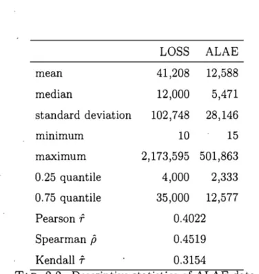
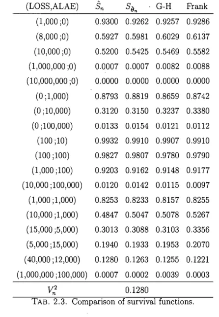
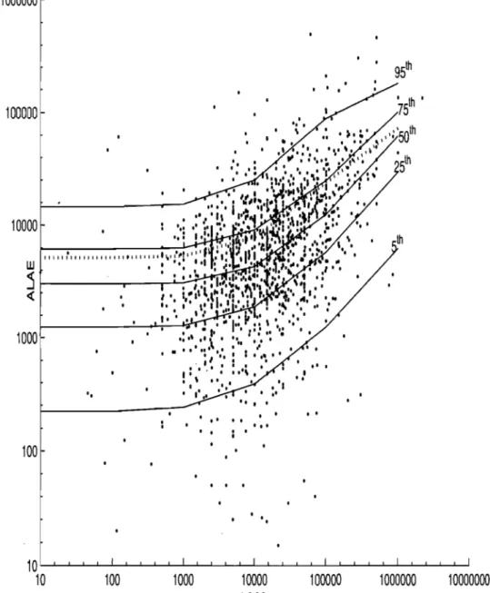
alors être comparés aux coefficients non paramétriques de 8pearman et de Ken-dall basés sur les rangs. Des valeurs rapprochées des coefficients paramétriques et non paramétriques sont une indication de la validité du modèle. Un test d'ajus-tement convergent est construit en comparant la fonction de survie paramétrique (bivariée) ajustée avec la fonction de survie expérimentale au travers d'une sta-tistique de type Cramér-von Mises. Ces résultats sont utilisés pour ajuster une distribution PH bivariée à un véritable jeu de données issu du domaine de l'assu-rance avec pour variables la perte subie (L088) et la dépense pour perte allouée après rajustement (ALAE). C'est la première fois à notre connaissance que les distributions PH bivariées sont utilisées sur de vraies données. La distribution

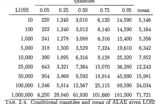
PH bivariée ajustée est ensuite utilisée pour calculer la moyenne et les quantiles de la distribution conditionnelle de la variable ALAE étant donné une valeur de l'autre variable L088.

Le deuxième article étend le théorème de Jewell en théorie de la crédibilité

à une grande classe de distributions qui sort des distributions exponentielles li-néaires et même de la famille exponentielle. Le théorème de Jewell montre que la crédibilité exacte se produit dans la famille exponentielle linéaire univariée et multivariée de distributions conditionnelles, une fois appareillées à la distribu-tion a priori conjuguée appropriée. La crédibilité exacte est étudiée ici dans le cas de distributions PH univariées et multivariées. Les chaînes de Markov sous-jacentes sont utilisées, en incluant les paramètres de risque non-observables pour les distributions PH.

MOTS CLÉS:

Distributions phase-type; processus de Markov continu; chaîne de Markov ca-chée; algorithme EM; bootstrap paramétrique; crédibilité exacte; distributions coxiennes; théorème de Jewell.

SUMMARY

Phase-type (PH) distributions are used as probability models for positive random variables. Their origin stems from the works of Neuts published in the early eighties. The first applications are found in operational research as models for waiting times in the field of queuing theory. Probability models in actuarial science are also fraught with positive variables such as losses and survival times which may explain the recent interest of actuaries in PH distributions. Stati~tical

estimation of PH distributions with the EM algorithm was developed in the mid nineties by Asmussen and his coworkers. Actuaries have also applied this class of models to risk theory and ruin probabilities. Extensions to multivariate PH distributions were also developed in the eighties following the seminal work of

Neu~s. They can serve as models for the joint probability distribution of two or' more positive random variables.

The first paper treats of maximum likelihood estimation by the EM algorithm and goodness-of-fit tests by parametric bootstrap when the model is a bivariate PH distribution. Âhlstrom and his coworkers published in 1999 an EM algorithm for the parametric estimation of relapse time distributions in survival analysis. They used a bivariate PH distribution with one component greater than the other component with probability one. Although the EM method proposed in this thesis is similar, our model is more general. Moreover, we show how to evaluate with any desired degree of accuracy the Spearman or Kendall corrrelation coefficients of the fitted bivariate PH model. These correlation coefficients can then be compa-red with the non parametric Spearman or Kendall coefficients based on ranks. A close agreement is an indication of the validity of the model. A consistent good-ness-of-fit testing procedure is proposed which compares the fitted (bivariate)

parametric survival function with the empirical survival function using a statistic of the Cramér-von Mises type. A parametric bootstrap algorithm is also provided to ob tain the critical region of the proposed test. The results are used to fit real data in the insurance industry relating losses (L088) and allocated loss adjust-ment expenses (ALAE). To our knowledge this is the first time ~hat bivariate PH distributions are used to fit real data. The fitted bivariate PH distribution is used to obtain the quantiles and the mean of the conditional distribution of the variable ALAE for a given value of the other variable L088.

The second paper extends Jewell's theorem in credibility theory to a larger class of distributions, outside of exponential distributions or even the linear expo-nential family. Jewell's Theorem proves that exact credibility occurs in the univa-riate and multivauniva-riate linear exponential family of conditional distributions, when paired with the appropriate conjugate prior distribution. Here, exact credibility is discussed in a univariate and multivariate PH setting. Hidden Markov chains are used, embedding the unobservable risk parameters in the PH distributions. KEYWORDS:

Phase-type distributions; continuous Markov pro cesses ; hidden Markov chain; EM algorithm; parametric bootstrap; exact credibility; coxian distributions; Je-well's theorem.

TABLE DES MATIÈRES

,

Sommaire. . . .. iii

Summary... v

Liste des tableaux. . . x

Liste des figures . . . xi

Remerciements . . . .. xiii

Chapitre 1. Preliminary notions on phase-type distributions and credibility theory. . . 1

1.1. Phase-type distributions. . . 1

1.1.1. Sub-intensity matrices and matrix exponentials . . . .. . .. . . .. . .. . 1

1.1.2. Continuous-time Markov chains. . . . .. . . .. . . .. . . .. . .. . . 4

1.1.3. Definition of phase-type distribution. . . 7

1.1.4. Properties of phase-type distributions. . . 9

1.1.5. Sorne examples of PH distributions ... , . . . .. . .. 12

1.1.6. EM algorithm for PH distributions.. .. .. .... .. .... . .. .... ... 15

1.2. Credibility Theory.. . .. . . .. . .. . . ... . . .. . . .. . .. . .. .. 19

1.2.1. Limited fluctuations credibility theory ... 20

1.2.2. Greatest accuracy credibility theory. . . .. 21

1.2.3. Exact credibility. . . .. 24

Bibliography. . . .. . .. 25

Abstract. . . .. 28

2.1. Introduction... . . . .. 28

2.2. Preliminaries... . . . .. 30

2.3. EM algorithm ... 33

2.3.1. General EM algorithm ... " . . . .. . . ... 33

2.3.2. EM algorithm for the BPH distribution ... " . .. 34

2.4. Simulated data from a BPH distribution. . . .. 39

2.5. Goodness-of-fit test. . . .. 42

2.6. Fitting ALAE data with a BPH mode!. ... 44

2.6.1. Conditional quantiles and mean. '" ... 47

Bibliograhy. . . .. 47

Appendix ...

~

50

Chapitre 3. Exact credibility with phase-type distributions. . . 56

A bstract . . . .. 56

3.1. Preliminaries on credibility theory . . . .. 57

3.1.1. Preview ... 57

3.1.2. Extensions... 60

3.2. Credibility theory for univariate PH . . . .. 64

3.2.1. Phase-type distributions. . . .. . . .. 64

3.2.2. Credibility theory. . . .. 66

3.2.3. Exact credibility for Coxian distributions. . . .. 70

3.3. Exact credibility for multivariate phase-type distributions. . . .. 72

3.3.1. Multivariate phase-type (MPH) distributions... 72

Bibliography. . . .. 75

Conclusion. .... .. ... ... ... .... ... 78

LISTE DES TABLEAUX

2.1 Bias and standard deviation of the EM estimator ... 41 2.2 Descriptive statistics of ALAE data. ... 44 2.3 Comparison of survival functions. . . . .. 46. 2.4 Conditional quantiles and mean of ALAE given LOSS ... " .... 48

LISTE DES FIGURES

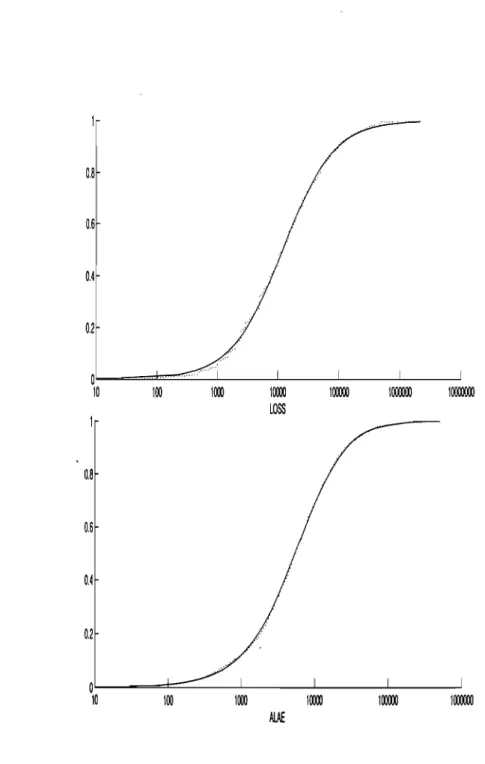
2.1 ALAE versus L088 with curves for conditional quantiles and mean. The dotted curve is the conditional mean of ALAE given L088. . . . .. 54 2.2 Marginal fitted distribution functions (smooth) and empirical distribution

To my family

A rash Jino

and Bayan

who offered me unconditionallove and sup-port throughout the course of this thesis.

REMERCIEMENTS

From the formative stages of this thesis, to the final draft, l owe an immense debt of gratitude to my supervisors, Martin Bilodeau and José Garrido. Their sound advice and careful guidance were invaluable throughout this entire thesis process. l also wish to thank Professor Bilodeau for financial support from his NSERC grant.

l would also like to thank to Professors Louis Doray, François Perron, Sabin Lessard, Charles Dugas, Manuel Morales, Richard Duncan, Christian Léger, Ale-jandro M urua, Roch Roy, Martin Goldstein and Anatole Joffe. AlI are faculty members of the Département de mathématiques et de statistique of Université de Montréal. Without their time and cooperation this thesis would not have been possible.

For their efforts and assistance, special thanks go as well to my friends Hir-bood Assa, Eugene Ursu, Zeinab Mashreghi, Romuald Hervé Momeya Ouabo and Mohammad Bardestani.

Finally, l cannot conclude without mentioning my brother Abdollah and his family, whose extreme generosity will be remembered always.

PRELIMINARY NOTIONS ON PHASE-TYPE

DISTRIBUTIONS AND CREDIBILITY

THEORY

1.1.

PHASE-TYPE DISTRIBUTIONS

1.1.1. Sub-intensity matrices and matrix exponentials

Suppose that the real matrix A

=

(aijkjEE, for E

=

{l, ... , l}, has eigenvalues Bi = Bi(A), i 1, ... ,i. Assume that

I(hl

~

IB21

~

...

~

IBd·

The following result is easily proved.

Lemma 1.1. If B = aA

+

b for sorne real constants a and b, then

The upper bound for the largest eigenvalue BI for a nonnegative matrix Îs given in the following lemma.

Lemma 1.2. Let A

=

(aijkjEE be a nonnegative rnatrix, i.e. aij ~ 0 for aU i,j, then,

Proof. If

4>

= (4)1, ... ,4>1) T is the eigenvector associated with BI, then

1

Bl4>i

=

L

aij4>j, i = 1, .. ') l,

and as a result 1 BIll <Pi 1 ~ 2::~=1 aij maxkEE 1 <Pk l, for i

=

1, ... ,l. Consequently, l

IBII max l<Pil _lEE

~

max _lEE

L

aij max l<Pkl· kEE

j=l

Thus IBII ~ maxiEE L::jEE aij. The proof simply uses the fact that AT has the

same eigenvalues as A. o

The density and Laplace transform of a phase-type distribution are expressed with a sub-intensity matrix. We present the required preliminaries of sub-intensity matrices;

Definition 1.1. The matrix T

=

(tij kjEE, is called a intensity or a sub-genemtor matrix if tij ~ 0, for i =J:. j, 2::~=1 tij ~ 0, and for at least one i E E,

2::~=1

tij

<

O.

The following lem ma gives an upper bound for the real part of the maximal eigenvalue of a sub-intensity matrix. Let ~(z) denote the real part of the complex number z.

Proposition 1.1. If T = (tijkjEE is a sub-intensity matrix then, the eigenvalues Bi(T;

=

0 or~(Bi(T;)

<

0, fori

=

1, ... ,l.

Proof. Let c

>

maxiEE(tii). Then, U = T+cI is a nonnegative matrix. Applying

Lemma 1.1 and Lemma 1.2 to the matrix U completes the proof. o

Because T = (ti,jkjEE is nonsingular if and only if Ois not an eigenvalue then,

we have the following corollary.

Corollary 1.1. A sub-intensity matrix T = (tijkjEE with eigenvalues Bi is non-singular if and only if ~(Bi( T;)

<

0, for i = 1, ... , l.

Definition 1.2. The exponential of a square matrix A is defined as

00 (tA)n

exp(tA) =

L -,-,

tE IR.

n=O n.

(1.1 )

In general, it is not an easy task to obtain the exponential of a matrix from the definition. There are many ways to caIculate the exponential of a matrix. Moler and Van Loan (1978), examines many ways to caIculate the exponential of a matrix to conclude that different forms of matrices require different approaches. The next theorem finds a representation formula for a matrix exponential.

Proposition 1. 2. Let

fh, ... ,

BI be the eigenvalues of A = (aij )i,jEE then,

exp(tA) = al (t)A_I

+ ... +

al(t)A1 (1.2)

where, ak(t) and Ak are given recursively by

al (t) = e'ht

,

Al = l, ak(t) =

1

t ellk_{(t-x)ak_1 (x)dx,} Ak = (A - BI!) ... (A - B_{k- 1}1), for k = 2, ... , l.

For a proof see Rolski et al. (1999), p. 325. We have the following coroUary from Proposition 1.2.

Corollary 1.2. Let BI,'" ,BI be the eigenvalues of A = (aijkjEE. Then, for each

s

>

maxiEE ~(BiL

Hm e- st exp(tA) = O.

t->oo (1.3)

Proof. In view of (1.2), we have ta show that Hm exp( -st)lak(t)1 = 0,

t ... oo (1.4)

for k

=

1, ...

J

Equation (1.4) is true for k

=

1. Suppose that (lA) holds for sorne k

=

n -

1

<

l. As a result, for each

e

>

0 there exists li

>

0 such that

exp(-sx)lan_l(x)1

<

e

for aU

x.>

li. On the other hand, we have that

e-stlan(t)1 $ e[!R(IJ,,)-slt

11/

le-IJnxan_1 (x)ldx

+

lt

e[!R(IJn)-Sj(t-X)e-SXlan_1 (x)ldx.

For a fixed point li

>

0, limt ... oo e[!R(lIn)-slt

f:

le-8nxan_1 (x)ldx =: O. This implies

that the first integrand tends ta zero. The second integrand is al ways less than

S-~(lIn)' and this completes the proof. 0

Let A(h)

=

(aij(h))i,jEE be a matrix function such that aIl its entries are differentiable functions of h. The matrix derivative of A(h) is defined by

dA(h)

=

hm A(h

+

b) - A(h) .

dh 5~O b . (1.5)

The following lemma states the derivative of a matrix exponential.

Lemma 1.3. The matrix exponential eAh is differentiable on the whole real line and

d Ah

_e _ _ A Ah _ AhA

dh - e - e . (1.6)

One can prove this lemma by using (1.1) and (1.5). For a proof, see Roiski et al. (1999), p. 315. If A and B are both differentiable matrix functions then, a differential rule for the product of A and B is given in the following lem ma. Lemma 1.4. If A(h) and B(h) are bath differentiable matrix functions then,

:h [A(h)B(h)]

=

[:hA(h)] B(h)

+

A(h) [:hB(h)] . (1.7)

As in the definition of the matrix derivative, the integral

J:

A(x )dx is a matrix with elements

J:

aij(x)dx, for 1/

<

t. In particular, for the matrix exponential function we have the following lemma.

Lemma 1.5. If T is a nonsingular matrix then,

l

t

exp(xT)dx

=

rI[exp(tT) - exp(1/T)]. (1.8)

M oreover, if all the eigenvalues of T have negative real parts then,

1

00

exp(xT)dx = -

rI.

Proof. Equation (1.8) is a consequence of (1.6) and (1.7) which imphes

Let 1/

=

a

in (1.8) and let s

=

a

in (1.3) to get limt~oo exp(tT)

=

O.

_o

1.1.2. Continuous-time Markov chains

Definition 1.3. A stochastic process

{J

t , t

2:

a}, defined on a probability space

(n,

J,

IP'), with values in a countable set E, called the space state of the process, is called a continuo us Markov chain if for any finite set

a

:S t1

<

t2

< ... <

tn

<

tn+l of times and corresponding set il, i2 , . . . ,in-l, i, j of states in E such that

P(Jtn

=

i, _{Jtn_l}

=

in-l, ... , _Jtl

=

id

>

0, we have

Equation (1.9) is called the Markov property. The Markov property states that in order to calculate the probability of a corning event given sorne past events, only the rnost recent past event is relevant. If for all s, t such that 0 ~ s ~ t and all i,j E E, the conditional probability _P(Jt = jlJs = i) depends only on t - s,

we say that the pro cess {Jl, t 2: O} is hornogeneous, or has stationary transition probabilities. In this case, IfD(Jt = j/Js

=

i)

=

IfD(Jt-s

=

j/Jo

=

i) and the function

Pij(t)

=

P(Jt

=

jlJo

=

i), i, j E E, t 2: 0

is called the transition function of the process. All continuous Markov chains dis-cussed in this thesis have stationary transition probabilities. The finite-dimensional probabilities of the pro cess {Jt , t 2: O} can be obtained in terrns of the transition

function Pij (t) and the initial probability distribution ai

=

IfD( Jo

=

i), i E E. In fact, we have

n

=

2:=

aio

II

Pim-l,im(tm - tm-d, ioEE m=l

where ta

=

O. As the transition function is also a conditional probability, it satisfies the following property :

It also satisfies

Pij(t) 2: 0, for aH i,j E E and 2:=Pij(t) = 1. jEE

Pij(O)

=

P(Jo

=

jlJo = i)

=

Oij

= {

1, 0,

i

=

j,

i

=1

j,

where 6ij is the Kronecker delta. Finally, for aU 8, t ~ 0, i, j E E,

Pij(t

+

s) = LPik(s)pkj(t). (1.11)

kEE

Equation (1.11) is called the Chapman-Kolmogorov equation. For a proof, see Anderson (1991). In order for the chain to go from state i to state j in time

t

+

8, it must be in sorne state at time 8. The Chapman-Kolmogorov equation

is obtained by using the Markov property and conditioning on the state at time s. The Chapman-Kolmogorov equation shows that if the transition function is known on sorne interval, 0

<

t

<

to, it is known for aH t

>

O. This fact suggests that the transition probabilities can be determined from their derivatives at O. If, for i

i=

j, the limit

q ..

=

lim Pij(h)

tJ h-+O h

exists then, % is called the jump rate from state i to state j. Note that the jump rate is not a function of

t.

This limit exists for aU the cases considered in this thesis. In general, it is possible to construct Markov chains based on jump rates, see Durrett (1999).

In the following, it is shown how to compute the transition probabilities from the jump rates. Using the Chapman-Kolmogorov equation (1.11),

Using (1.10), note that 1 - Pii(S) = Ek;6iPik(8), 50 that Hm _Pl_ï (_8 ) _ _ 1 = _ lim

~

P_ik_( 8_) = - " " qik

8-+0 8 II-+O~ 8 ~

k;6i k;6i

The limit as 8 goes to

a

of (1.12) is

p~/t) = LqikPkj(t) - ),iPij(t). k;6i

(1.12)

(1.13)

Introducing the matrix Q = (qij) , where qii = -),il equation (1.13) may be

rewritten in matrix form for p(t) = (Pij(t))ij as p' (t) = Qp(t).

This is Kolmogorov's backward equation. This equation solves for

The rnatrix Q is called the infinitesirnal generator of the Markov chain. Anderson (1991) gives a rigorous account of continuous-tirne Markov chains.

1.1.3. Definition of phase-type distribution

A random variable that is defined as the absorption time of an evanescent finite-state continuous-time Markov chain is said to have a phase-type (PH) dis-tribution. The distribution and density functions of a PH distribution can be expressed in terms of the m x 1 initial state distribution vector 7r and the m x m infinitesimal generator matrix T of the underlying Markov chain. The pair (7r, T) is known as a representation of order m of the PH distribution. Since their in-troduction by Neuts (1981), PH distributions have been used in a wide range of stochastic modeling applications in areas as diverse as telecommunicatiollS, tele-traffic modeling, biostatistics, queueing theory, risk theory, reliability theory, and survival analysis. Erlang (1917) wrote the first paper to extend the familiar expo-nential distribution with his method of stages. He defined a nonnegative random variable as the time taken to move through a fixed number of stages, spending an exponential amount of time with a fixed positive rate in each one. Nowadays, we refer to distributions defined in this manner as Erlang distributions. Cox (1955) generalized Erlang's notion by allowing complex parameters. This construction, defines the class of distributions with rational Laplace-Stieltjes transforms (LST), of which the class of PH distributions is a proper subset. These distributions are nowadays also known as matrix-exponential distributions. Neuts (1981) genera-lized Erlang's method of stages in a different direction. He defined a phase-type random variable as the time taken to progress through the states of a finite-state evanescent continuous-time Markov chain, spending an exponential amount of time with a positive rate in each one, until absorption.

PH distributions have many appealing features. In the following sorne of them are listed.

(1) They are dense in the class of aU distributions defined on the nonnegative real numbers.

(2) The use of PH distributions in stochastic models often enables algorith-mically tractable solutions to be found. Quantities of interest, such as the distribution and density functions, the Laplace-Stieltjes transform, and the moments of PH distributions are expressed simply in terms of the ini-tial phase distribution 1T and the exponential or powers of the infinitesimal

generator T.

(3) Stochastic models, particularly where the exponential distribution is used to model quantities (such as inter-arrivaI times, service times, or lifetimes), can now be extended with PH distributions.

(4) Since the class of PH distributions is closed un der a variety of operations, such as finite mixtures and convolutions, systems with PH inputs often have PH outputs.

Neuts and his coworkers, in the late seventies, established much of this mo-dern theory. Neuts (1995) developped queuing theory by PH distributions and Asmussen (2000) applied PH distributions to risk theory.

Let {Jt , t ~

O}

be a Markov process in the finite state space

E = {1, ... , m, m

+

1} ,

where 1,2, ... , mare transient and, thus, m

+

1 is an absorbent state. Then, {Jt , t ~

O}

has an infinitesimal generator of the form

(1.14)

where T

=

(tij)i,j=l, ... ,m is an m x m matrix, t = (ti)i=l,.",mis an m dimensional

column vector and 0 is an m dimensional vector of zeros. Superscript T stands for the transpose of a matrix or vector. Since the rows of an infinitesimal generator must sum to zero, note that t

=

-Te, where e

=

(1,1, ... , I)T is the vector of ones. Let ai IP( Jo = i) be the initial state probabilities. Often, it is assumed that the chain does not start in the absorbent state, i. e. am+l

=

O. In that case,

Ct can be written as

This condition is assumed in the next definition.

Definition 1.4. The time until absorption,

x

=

inf {t ~

01

Jt

=

m

+

1} (1.15)

is said to have a PH distribution with representation or parameters (Tr, T). The dimension m of Tr is said to be the dimension of the phase-type distribu-tion.

1.1.4. Properties of phase-type distributions

The first property relates to the exponential of the infinitesimal generator matrix.

Proposition 1.3. Assume the representation (1.14) of the infinitesimal genera-tor. Then,

Proposition 1.4. If X has a PH distribution with parameters (Tr, T) then, the density of X is given by

Proof: Let Pij(X)

=

IP(Jx

=

jlJo

=

i). Then,

m m m m

i=1 j=1 i=1 j=1

where (eTx)ij is the ij-element of the eTx . The density function is the derivative of the cumulative distribution function. Renee, f(x)

=

Tr T eTxt.

Proposition 1.5. The Laplace transform of X is given by

where l is identity matrix of dimension m.

From the definition of the inverse of a matrix, one can write the LST as a ratio of polynomials. The maximum degree of the denominator is m and the degree of the numerator is less than m (because the limit of the Laplace transform as s

goes to -00 is zero). Then, it can be written as foUows

L(s)

=

1 + ClS

+ ... +

Cm_lSm -1 1

+

dIS

+ '" + dms m

Phase-type distributions not only have rational Laplace transforms, but also with sorne conditions aU distributions with rational Laplace transform are of phase-type. See the following theorem of Q'Cinneide (1989).

Proposition 1.6. A distribution defined on [0,00) is a PH distribution if and only if

(1) it is the point mass at zero, or

(2) a): it has a strictly positive density on (0,00), and

b): it has a~ rational Laplace transfo Tm such that there exists a pole of

maximal real part, -" that is real, negative, and such that - ,

>

~( -ç-), where ~(-ç-) is the real part of any other pole. Proposition 1.7. The moment of arder n, n ~ 1, of X is given by

As a consequence, the full class of PH distributions of order m has a

parame-trization in 2m - 1 dimensions. This foUows from the Cayley-Hamilton theorem from which there is at least one sequence >'0, >'1,"" >'m-l such that

m-l

T-me

=

L

>'iT-ie.

i=O

If we fix such a sequence then, those coefficients together with the first m - 1 moments de termine all the moments recursively. lndeed, it can be seen by pre-multiplying the relation ab ove by -rrT-n that

(-l)~+mJE [xn+m] m-l (_l)n+iJE [xn+i]

(n

+

m)!

=

~

>'i (n

+

i)! .

Since the Laplace transform near zero is determined by aU the moments, it follows that >'0, >'1, ... ,>'m-l and JE

[X] , ...

,JE [X m-1] determine the distribution.

When the representation of the PH distribution is estimated, overparametri-zation will occur. From the latter discussion, a PH distribution of dimension m has a parametrization with 2m - 1 parameters. However, direct estimation of the representation (rr, T) requires m2

+

m - 1 parameters to be estimated.

Neuts (1981) showed that the convolution of two independent PH variables with possibly different dimensions is a PH variable.

Proposition 1.8. Suppose that F and G are PH distributions with representa-tions (a, T) of orderm and ({3, S) of ordern, respectively. Then, their convolution F

*

G is a PH distribution with representation

h,

R) of order m

+

n, where

and t

= -

Te.

R = ( T

-t{3T) ,

o

-8

l':l'0te that F(O) is the probability that the chain associated with F starts in

the absorbent state, i. e. F(O) = Gm+l' It is also easily proved that a finite mixture of PH distributions follows a PH distribution.

Proposition 1.9. If (Pl j . . . ,Pk) is the vector of mixing probabilities and Fj is a

PH distribution with representation

(7r

j, T_{j ),} 1 ::; j ::; k, then, the mixture has the representation with initial state probabilities

Pk7r_k

and infinitesimal generator

Tl 0 0

0 T2 0

T=

0 0 _Tk

Definition 1.5. A PH distribution is called triangular phase-type, or TPH, if it has a representation in which the matrix T is of infinitesimal genemtor upper triangular.

The most important property of TPH distributions found in Assaf and Le-vikson (1982) is that absorption happens in a bounded number of transitions. Proposition 1.10. The TPH class of distributions is the smallest class contai-ning all exponential distributions and which is closed under finite mixtures, finite convolutions and formation of coherent systems.

1.1.5. Sorne exarnples of PH distributions

In the following, sorne well-known probability density functions are represen-ted by phase-type distributions. More examples can be found in Fackrell (2003).

Exarnple 1.1. The exponential distribution with density function f(x)

=

Àe-'\x has the representation

7r = 1,

T = -À.

Example 1.2. The hyper-exponential distribution with probability density function

n

f(x) =

L

aiÀie-'\;x

i=l has the representation

-À₁ 0 0

o

T

o

o

Example 1.3. The rn-phase Erlang distribution with density function

has the representation 7r - (l,O, ... ,O)T,

->. >.

0

->.

T = 0 0 0 0

where m is the dimension of Matrix T.

0

>.

0 0

o

0

o

0

->. >.

o

->.

Example 1.4. A PH distribution is unicycle if it has a representation of the form

7r

=

(Œl,Œ2, ... ,Œm)T, ->'1 >'1 0

o

0 0 ->'2 >'2

o

0 T

₌

0 0 0 ->'m-l >'m-l /-LI /-L2 /-L3 /-Lm-l

->'m

where, for i = 1, ... , m - 1, /-Li 2: 0, >'1 ::; >'2 ::; >'3 ::; ... ::; >'m and >'m

>

E:,~l /-Li·

In the next example it is exemplified that the representation of a phase-type dis-tribution may not be unique.

Example 1.5. In the folIowing example from Botta et al. (1987) the non-uniqueness of the representation happens even for the minimal order or dimension of a PH distribution. AlI the next three representations lead to the same PH probability density function

The representations are

7r = (1/3,2/3) T and T =

7r

=

(1/5,4/5) T and T

=

(

-~

-~

),

(1.17)

and

-3 1 1

7r

=

(0,1/2,1/2) T and T

=

1 -4 2 (1.18)

1 0 -6

In the representations (1.16) and (1.17), the or der of the PH distribution is 2, whereas it is 3 in (1.18). In general, a representa,tion which has the minimum order is called minimal. From this example, even the minimal one is not unique. The order of a PH distribution is defined as the order of the minimal one

Example 1.6. A PH distribution is said to be acyclic if its matrix T is upper

triangular.

Example 1.7. A PH distribution is said to be Coxian of order p if

7r - (I,O, ... ,O)T, -À 1 q1À1 0

o

0 0 -À2 q2À2

o

0 T 0 0 0 - Àp- 1 qp-1Àp - 1 0 0 0

o

-À_p

w here 0

<

qi

<

1 and Ài

>

0, i = 1, ... ,

p'-As in Proposition 1.6, we have the following theorem about the characterization of Coxian distributions.

Proposition 1.11. A distribution defined on [0,00) is a Coxian distribution if and only if

(1) it is the point mass at zero, or

(2) a): it has a strictly positive density on (0,00), and

b): it has a rational LST with only real and negative poles.

See O'Cinneide (1991) for a proof. A remarkable result from Cumani (1982) and Dehon and Latouche (1982) establishes that a PH variable having an acyclic

Markov chain representation can be uniquely represented by a Coxian distribution with stochastically increasing states, i.e.

->'1 ::; ->'2 ::; ... ::;

->'p,

Such pro cesses start at state 1 and can only jump from i to i

+

1 or p

+ 1.

Therefore, the true parameter dimension is 2p - 1, where p is the dimension of the acyclic PH distribution.

1.1.6. EM algorithm for PH distributions

The EM (Expectation-Maximization) algorithm of Dempster et al. (1977) is a general iterative method for finding the maximum-likelihood estimate of the parameters, when the data is incomplete or has missing values. It finds its useful-ness when the likelihood function of the incomplete (observed) data is intractable but that of the complete (unobserved or missing) data lS of a simpler form which can be analytically optimized. Assume that the data x is observed and generated by sorne distributions, say f(xl1» with log-likelihood function l(1))

=

logf(xl1». We calI x the incomplete data and refer to l(1)) as the incomplete log-likelihood function. Suppose that an unobserved (complete) data y, where x = x(y), has

pdf g(yl1». Assume

Q(1)'I1>) = 1Eq, [logg(yl1>') lx]

exists for aU pairs (</J',</J). The EM iteration 1>(p) ~ 1>(p+l) is defined as follows: E-step : Compute Q(1)I1>{p)).

M-step : Find </J(P+1) that maximizes Q( 1>11>{p)) over 1>.

Simplifications occur when the complete datà density function is a member of the exponential family

g(yl</J) = b(y) exp [1>T t (y)] /a(</J), (1.19)

where 1> is the vector parameter, t(y) is the vector of the complete data sufficient statistic. If (1.19) holds, simplified expressions found in Dempster et al. (1977) for the E and M steps are : E-step : Estimate the complete data sufficient statistics t(x) by finding

M-step : Determine 4J(p+l) as the solution for 4J of the equation lE</> [t(y)]

=

t(p).

By definition a PH random variable is the time until absorption in an ab-sorbent state. This can be considered as an incomplete data in the sense that they only provide information about the absorption time of the absorbent state, not about the whole path of the underlying Markov chain, Jt . The initial state, the states that have been visited, and the time spent in each visited state are not observed. Renee, the hidden information can help to maximize the incomplete likelihood function which is untractable. For an observation x from a PH va-riables as defined in (1.15) with representation (7r, T), the complete information is formulated by the embedded Markov chain of visited states

and the sojourn times

where k is the number of jumps until hitting m

+

1. A complete observation of the process Jt on the interval (0,

x]

is represented by

y = (io, ... , ik - 1 , Sa,···,

sk-d,

where x

=

sa + ... + Sk-l. To get the probability density function of y, one needs the probability Pjl of jumping from j to l which is given by

0, j,l

=

1, ... ,m,j

=

l,

Pjl

=

lP'(in+l

=

llin

=

j) = ..!.i..!..-- t j j ' j,l

=

1, ... ,m,j =1= l,

it" ,

j

=

1, ... , m, l

=

m

+

1.

- j j

The density of y can be derived by Markov chain properties and considering that the time spent in each state i has an exponential distribution with mean 1/ ).,i, where ).,i

=

-t_{ii ,} as in Asmussen et al. (1996). Thus,

(1.20) where f)

=

(7r, T) is the parameter.

Let JP], ... , Jin] be n independent realizations of the process. This gives n

embedded Markov chains

.[11] .[11]

'1,0 , ... , 2kllll_1'

with corresponding holding times

[II] [II]

so , ... , skllll_1'

The complete data becomes y

=

(y[l], ... , y[n]), where

[II] _ ('[11] .[11] [II] [II]) - 1

Y - '1,0 , ... ,2kllll_1'SO , ... ,skllll_1' 1 / - , . . . ,n.

The observed incomplete data is the following function of the complete data

X[II]

=

(S[II]

+ ... +

S[II] )

o kllll-I . Define 1 { '1,0 '[IIJ -- '1, .} , k11l1 -I

2: 1

{it

J ₌

i}

_st], ... =0 Let n Bi =

2:

B₂ !II] _, 11=1 n Zi

2:

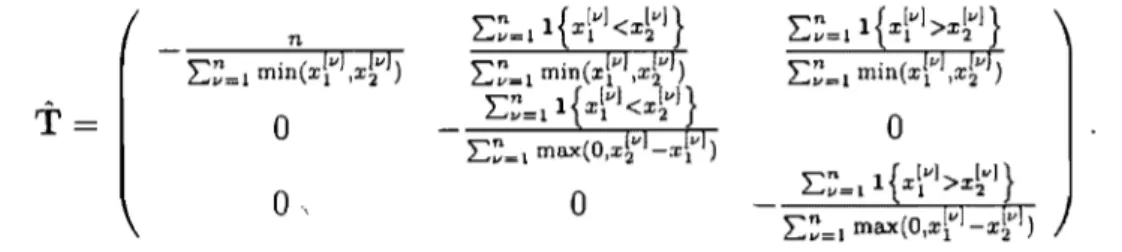
Z₂ !II] _, 11=1 n Nij = 2:NI~J _{2J '} 11=1

be the number of Markov processes starting from state i, the total time spent in each state i, and the number of jumps from state i to state j, respectively. Then, the density of the complete data y is the product of n densities as in (1.20)

where ti,m+l ti . The density (1.21) is a member of a curved multi-parameter

exponential family with sufficient statistics

where i l, ...

,m,

j = l, ... ,m

+

l, i

i=

j. The M-step is given by

The E-step for an exponential family consists of computing the conditional ex-pectation of the sufficient statistics, given the complete data and the current parameter estimates. If the current parameter estimates at step h of the algo-rithm is (J(h), the complete sufficient statistics at the h

+

1 E-step consists in the

evaluation of the following conditional expectations

n

I::

IEe(l»

[BIll)

IX[II]] )

11=1 n

2:

IEe(l»

[zlll]lx[II)] )

11=1 n

2:

IEe(l»

[Nl;llx[II)] )

11=1

for i l, ... ) m, j = l, ... , m

+

l, i

i=

j. The E-step is the most complicated step. It is given in details in Asmussen et al. (1996). Define

e(a , b , i , J' , T) = l b e T(u-a)K·e T(b-u) l ] , du

a

where Eij is an m x m matrix with a one in position (i, j) and zeros elsewhere.

where 7T~h) is the ith component of 1i(h) ,

1i(h)T C(O

_,

x[vl i i _{" ,} T(h))e

f(x[v1IO(h))

t .. 1i(h)T C(O, x[v] , i, j, T(h))e

- tJ f(X[v1iO(hl ) ,

where i,j = l, ... ,m, i =f j. The function C(a,b,i,j,T) can be evaluated by numerical methods in ordinary or partial differential equations su ch as the Runge-Kutta method of order four. More detailed useful numerical methods can be found in Asmussen et al. (1996).

1.2.

CREDIBILITY THEORY

Generally speaking, credibility theory is a quantitative tool that allows an insurer to combine the past experience of a policyholder to the pure premium in a risk class or group of risk classes. If the past observed experience of the policyholder indicates a difference in risk to that assumed for the class, then the insurer has to explore this difference to see if it is due to a really different policyholder or it is only due to natural stochastic variation in the risk cIass. If the policyholder is indeed different, then sorne credible information can be obtained from the individual experience which is not being considered when the pure premium or manual premium is calculated. In other words, the assumption of homogeneity in the risk cIass fails.

For example, in car insurance the insurer may assume that the number of accidents in one year follows a Poisson distribution with mean f.l, but then the experience of a particular policyholder may have an average

X

that is far from

f.l. In statistical term,

X

would show a significant difference with f.l. In this case, the insurer must consider two facts :

(1) The risk class is not homogeneous. Its heterogeneity should be taken into account.

(2) What share of this difference is due to heterogeneity and to natural ran-dom variation?

To combine these two facts, the credibility premium, Pc should be a combination of the manual rate M and the past individual observation summary

X.

A very good candidate for Pc is

Pc = ZX

+

(1 - Z)M , (1.22)

where the credibility factor Z E [0,1] should be determined. Full credibility occurs when Z 1. Section 1.2.1 deals with limited fluctuations credibility theory which developed at the beginning of twentieth century and represented a first attempt to model credibility in practical situations. The problem with this approach is its lack of a sound underlying mathematical theory justifying the method. As a result, greatest accuracy credibility was developed. It is introduced in Section 1.2.2. This method provides a statistical framework for credibility theory, where the risk parameter has a prior distribution modelling the, possible heterogeneity within the portfolio. Both, the classical models of Bühlamnn and Bühlamnn-Straub will be discussed.

1.2.1. Limited fluctuations credibility theory

Limited fluctuations credibility theory was developed in the early part of twen-tieth century as the first attempt to give quantitative credibility rules. Suppose that XI, . .. , Xn represent the past daim experience of a policyholder and are i. i. d., with theoretical mean fJ- and variance (J'2. The variance of

X

=

L.j~l

Xj is

n . In this limited fluctuations approach if the variation of

X

about fJ- is not si-gnificant, then full credibility is assigned to

X.

In statistical terms, it means that the difference between

X

and fJ-is small relative to fJ- with a high probability, i.e., for gi ven small rand 0

<

p

<

1 (with r close to 0 and p close to 1)

then full credibility occurs if

~

<

I!i

ft - V~'

where

>'0

=

(M;Y.

For more details see Klugman et al. (2008), p. 558.

When full credibility does not hold, the linear credibility premium (1.22) is deemed appropriate. One good choice for Z in (1.22) is

n n+k'

where n is the number of observations in

X

and k is a constant to be chosen. This form of Z tends to 1 as n --+ 00. A very elementary way to determine Z in (1.22) is to force the variance of the premium Pc in (1.22) to be controlled at a

2 •

level, say

fa.

In thlS case Z can be expressed by the formula

For more details on limited fluctuations credibility theory see Norberg (1979), Mowbray (1914), Herzog (1999) or Longley-Cook (1962).

1.2.2. Greatest accuracy credibility theory

Greatest accuracy credibility theory is a model-based approach introduced by Bühlmann (1967). In this approach, the risk parameter 8 is modeled by a probability distribution, say II. The values of 8 varies for different policyholders and this random nature of 8 reflects the heterogeneity within an insurance port-folio. For a given 8 = 0 the distribution of the number or size of daims in year i = 1, ... , n

+

1 is given by !x;I(}(x 1 0). Usually it is assumed that for a given 0,

the Xl,'" 'Xn+l are i.i.d. random variables.

The ideal premium rate for the next year n+l should be ftn+l (8)

=

lE [X_{n + l} 18], but the value of 8 is not known. In a Bayesian context, lE

[X

n+l 1 Xl, ... , X_{n ]} is a

valuable substitute with desirable properties. Mathematically, there is no dosed form formula for this Bayesian premium, except for sorne special combinations of the prior distribution, II and !XI8=(}(X 1 0). Bühlmann (1967) approximates

lE

[X

n+1 1 8l by a linear function of the past observations Xl, ... ,X_n with a

pre-mium formula of the form :

n

ao

+

Laixi,

j=l

where O:j, for j

=

1, ... ,n need to be determined. To this end, the o:'s are chosen

such as to minimize the squared error loss, that is

where the expectation is taken over the joint distribution of _{Xl, ... ,Xn} and 8. Equating ~ to 0 yields the estimators aj which satisfy

n

lE[ILn+1(8)]

=

lE[Xn+1]

=

ao

+

L ajlE[Xj ] , j=l

(1.23)

while by taking the partial derivative of Q with respect to ai and setting to 0 gives

n

lE[ILn+1(8)Xi]

=

aolE[Xi ]

+

L ajlE[XiXj ]. j=l

The left-hand side of this equation can be written as

Thus 8Q/8ai = 0 implies

lE {I~[ILn+1 (8)Xi I8]) lE _{{ILn+1 (8)lE[Xi} 18]} - lE {lE[Xn+118]lE[XiI8]}

= lE {I~[Xn+1XiI8]}

n

lE[XiXn+d = oolE[Xil

+

L 0)8: [XiXJl, j=l

Multiplying (1.23) by lE[Xd and subtracting from (1.24) we have

n

(1.24)

Cov(Xi,Xn+d

=

LOjCov(Xi,Xj ), i = 1, ... ,n. (1.25)

Equations (1.23) and (1.25) together are called normal equations. In the

sim-plest case, it is assumed that given 8 = 0, the Xl, ... ,Xn+l are i. i. d. random variables. Define

and

where j.L(0) and 11(0) are referred to as the hypothetical mean and pro cess variance, respectively. Define also

and

Bühlmann (1967) shows that n j.L = lE[j.L(8)] , Il = lE[II(8)] , a

=

V(j.L(8)]. Qo

+

LQjXj = ZX

+

(1- Z)j.L, j=l n

where Z = - - k and k is given by

n+

k

=

~

=

lE[V(Xj _I8)]

a V[lE(XjI8)]'

(1.26)

The value of Z derived from (1.26) is known as Bühlmann's credibility factor. The values Qo, QI,"" Qn also minimize

and

(1.28)

To see this, take derivatives of (1.27) or (1.28) with respect to aD, al, ... ,an and note that the solutions still satisfy the normal equations (1.23) and (1.25). Hence the credibility premium Qo

+

~;=l QjXj is the best linear estimator of each of the hypothetical me an lE [Xn+ 1 18] , the Bayesian premium lE[Xn+lIXl , ... ,X_{n ]} and

In Bühmann-Straub's credibility theory model, the classic Bühmann's 8S-sumptions are generalized. In this model the conditional variance, V[Xj

le

=

8l

is allowed to be a proportional to v(8), i.e.

but still IE[Xjle =

8l

does not depend on j. As a result we have again n

ŒO

+

L

ŒjXj

=

ZX

+

(1 - Z)J.L, j=l

where

X

=

_{LJn_l '!!!:iXJ., Z}

=

~,m

=

ml

+ ...

+mn and k is given by (1.26).

- m m+k

For more details on Bühlmann-Straub's model see Klugman et al. (2008), p. 588, or Bühlmann and Gisler (2005), p. 77.

1.2.3. Exact credibility

Mayerson (1964) finds that the linear credibility premium is the exact Baye-sian premium for some combinations of prior (also called structural) and claims distributions. Jewell (1974) extends these exact credibility results to the univa-riate exponential family of distributions with a proper choice of prior. His main result is a special case of the following theorem.

Proposition 1.12. (Linear Exponential Family) Suppose that the Xn in X =

(Xl, ... ,XN+l ) Tare conditionally independent, given

e,

with common probability

density function

Xj E X,8 E

n,

(1.29)

and the prior density is a natural conjugate [q( 8)] -k ell k r(fJ)r' (8)

1['(8)

=

c(J.L, k) , (1.30)

where -00 ~ 80

<

81 ~ 00, with 1['(80 )

=

1['(81)

=

0, J.L

=

IE(X) and k

=

~~i~:~ll, then exact credibility occurs, with

(1.31)

For a proof see Jewell (1974) and Klugman et al. (2008) p. 593.

Landsman and Makov (1998) extends Jewell's Proposition 1.12 to the larger exponential dispersion family. In a parametrization similar to that of Klugman et

al. (2008), p. 593, its probability density functions are written as :

p(>. x) eÀr(8)x

fXle(xIB) = [q(B)]À ' xE X,B E

n.

(1.32)

The introduction of the dispersion parameter

>.

makes this a more flexible family of distributions than the linear exponential family

(>'

= 1). The natural conjugate prior on 8 remains the same as in (1.30) and exact credibility still occurs, now with Z

=

À~k' Other properties of (1.32) are that j.L(B)

=

IE(X 1 8

=

B) =

q'(B)j[r'(B)q(B)] and (J2(B)

=

V(X 1 8

=

B)

=

j.L'(B)/[>.r'(B)]. Using the natural

conjugate in (1.30) gives j.L

=

IE[j.L(8)] and k

=

IE[V(XI8)]jV[IE(XI8)]. For a comprehensive treatment on the exponential dispersion family, see Tweedie (1984), Nelder and Wedderburn (1972) or J(ZIrgensen (1987).

B

IBLI OG RAPHY

Anderson, W. J. (1991). Continuous-time Markov chains. Springer-Verlag : New York.

Asmussen, S., Nerman, O., Olsson, M. (1996). Fitting phase-type distributions via the EM algorithm. Scand. J. Stat. 23, 419-441.

Asmussen, S. (2000). Ruin probabilities. Advanced Series on Statistical Science &

Applied Probability, 2. World Scientific Publishing Co., Inc., River Edge, NJ. Assaf, D., Levikson, B. (1982). Closure of phase type distributions under operations

arising in reliability theory. Ann. Probab. 10, 265-269.

Botta, R. B., Harris, C. M., Marchal, W. G. (1987). Characterizations of generalized hyperexponential distribution functions. Stochastic Models 3, 115-148.

Bühlmann, H. (1967). Experience rating and credibility. ASTIN Bull. 4, 199-207. Bühlmann, H., Gisler, A. (2005). A course in credibility theory and its applications.

Springer-Verlag : New York.

Cox, D. R. (1955). A use of complex probabilities in the theory of stochastic processes. Proc. Cambridge Philos. Soc. 51, 313-319.

Cumani, A. (1982). On the canonical representation of homogeneous Markov pro-cesses modelling failure time distributions. Microelectronics and Reliability 22,

583-602.

Dehbn, M., Latouche, G. (1982). A geometric interpretation of the relations between the exponential and generalized Erlang distributions. Adv. in Appl. Probab. 14,

885-897.

Dempster, A. P., Laird, N. M., Rubin, D. B. (1977). Maximum Iikelihood from incomplete data via the EM algorithm. J. Roy. Statist. Soc. Ser. B. 39, 1-38.

Durrett, R. (1999). Essentials of stochastic processes. Springer-Verlag : New York.

Erlang, A. K. (1917). Solution of sorne problems in the theory of probabilities of significance in automatic telephone exchanges. The Post Office Electrical Engi-neer's Journal 10, 189-197.

Fackrell, M. W. (2003). Characterization of matrix-exponential distributions. PH. D.

thesis : The University of Adelaide.

Herzog, T. (1999). Introduction to credibility theory, 3rd ed. Winsted, CT :ACTEX.

Jewell, W. S. (1974). Credible means are exact Bayesian for exponential families.

ASTIN Bull. 8, 77-90.

J0rgensen, B. (1987). Exponential dispersion models, with discussion and a reply by the author. J. Roy. Statist. Soc. Ser. B. 49, 127-162.

Klugman, S. A., Panjer, H. H., Willmot, G. E. (2004). Loss models : From data to decision. Third edition. John Wiley & Sons: Hoboken, NJ.

Landsman, Z. M., Makov, U. E. (1998). Exponential dispersion models and credi-bility. Scand. Actuar. J. 1, 89-96.

Longley-Cook, 1. (1962). An introduction to credibility theory. Proceedings of the Casualty Actuarial Society XLIX, 194-221.

Mayerson, L. (1964). A bayesian view of credibility. Proceedings of the Casualty Actuarial Society 51, 85-104.

Moler, C., Van Loan, C. (1978). Nineteen dubious ways to compute the exponential of a matrix. SIAM Review 20, 801-836.

Mowbray, A. H. (1914) How extensive a payroll exposure is necessary to give a dependable pure premium? Proceedings of the Casualty Actuarial Society l, 24-30.

Nelder, J. A., Wedderburn, R. W. M. (1972). Generalized Linear Models. Journal

of the Royal Statistical Society. Series A (General) 135, 370-384.

Neuts, M. F. (1981). Matrix-geometric solutions in stochastic models. An

algorith-mic approach. Johns Hopkins University Press, Baltimore, Md.

Neuts, M. F. (1995). Matrix-analytic methods in queueing theory. Probab.

Stochas-tics Ser.) 265-292. Boca Raton, FL.

Norberg, R. (1979). The credibility approach to experience rating. Scand. Actuar. J. 4, 181-221.

O'Cinneide, C. A. (1989). On nonuniqueness of representations of phase-type dis-tributions. Comm. Statist. Stochastic Models 5, 247-259.

O'Cinneide, C. A. (1991). Phase:'type distributions and majorization. Annals of

Applied Probability 1, 219-227.

O'Cinneide, C. A. (1999). Phase-type distributions: open problems and a few properties. Comm. Statist. Stochastic Models 15, 731-757.

Roiski, T., Schimdli, H., Schmidt, V., Teugels, J. (1999). Stochastic processes for

insurance and finance. John/Wiley & Sons.

Tweedie, M. C. K. (1984). An index which distinguishes between some important exponential families. In Statistics : Applications and New Directions. Proceedings

of the Indian Statistical Institute Golden Jubilee International Conference. (Eds. J.K. Ghosh and J. Roy), Calcutta: Indian Statistical Institute, 579-604.

FITTING BIVARIATE LOSSES WITH

PHASE-TYPE DISTRIBUTIONS

This paper was submitted for publication in February 2009 to the North Ame-rican Actuarial Journal which is a refereed journal. The first author is Amin Hassan Zadeh and the coauthor is his Ph. D. supervisor Martin Bilodeau.

ABSTRACT

Maximum likelihood estimation and a (parametric bootstrap) goodness-of-fit test are considered for bivariate phase-type distributions. The initial probability vector and infinitesimal generator matrix are estimated by the EM algorithm. In a special case, the dependence structure of bivariate phase-type distributions is revealed. The results are used to fit a real bi-dimensional data set related to insurance losses (L088) and aIlocated loss adjustment expenses (ALAE). The fitted bivariate phase-type is used to obtain conditional quantiles and mean of ALAE for a given value of L088. The bivariate phase-type distribution meets aIl the requirements listed in Klugman and Parsa (1999).

Key words : Bivariate insurance losses, bivariate phase-type distribution, conti-nuous Markov process, EM algorithm

2.1.

INTRODUCTION

Phase-type (PH) random variables are defined as the time until absorption in a set of absorbent states in a continuous time Markov chain environment. Coxian,

Erlang-n, hyper-exponential and mixture of Erlang-n distributions are special cases of PH random variables. Neuts (1981) defines the PH random variable and establishes its theoretical properties. PH distributions are dense among aU distri-butions with positive support. In addition, they have density, Laplace transform and aU their moments in closed form and thus, various probability quantities can be obtained easily. Despite the interesting properties of PH variables, sorne diffi-culties arise in statistical estimation. Non-uniqueness of representations in sorne PH models, as discussed in O'Cinneide (1989), and over-parametrization is brie-fly mentioned in Asmussen et al. (1996). Asmussen et al. (1996) study parameter estimation by the EM algorithm, as weU as fitting other densities on the positive line with PH distributions. In Assaf and Levikson (1982) sorne properties of PH variables in reliability are investigated. Asmussen (2000) applies PH distributions to risk theory. In Drekic et al. (2004), the distribution of deficit at ruin, in the Sparre Andersen renewal model, with PH distributed claim size is considered. Li and Garrido (2004) consider the ruin probability in risk theory for Erlang-n distri-butions, a special case of PH distributions. In Assaf et al. (1984), a multivariate PH distributions is defined. In Kulkarni (1989) a new class of multivariate PH distribution is introduced. In the multivariate case, the structure of dependence under sorne conditions is studied by Li (2003). The conditional tail expectation for multivariate PH distributions is obtained in Cai and Li (2005a).

This paper is organized as follows. Univariate and multivariate PH variables, with their properties, are briefly defined in Section 2.2. Section 2.3 covers para-meter estimation of bivariate PH (BPH) distributions via the EM algorithm. In Section 2.4, a method to simulate a BPH distribution is used in a smaU simula-tion study on the bias and standard deviasimula-tion of the EM estimator. A (parametric bootstrap) goodness-of-fit test for BPH distributions is proposed in Section 2.5. Section 2.6 includes a data analysis of the ALAE data by fitting a BPH distribu-tion. It also gives expressions for the conditional quantiles and condition al mean. This article extends the works of Asmussen et al. (1996), Assaf et al. (1984) and Âhlstrom et al. (1999) to problems of statistical nature in BPH distributions,