Visual urban space assessment from sky shape
analysis
François Sarradin
1, Daniel Siret
1, Jacques Teller
21CERMA UMR CNRS 1563
School of Architecture of Nantes rue Massenet – BP 81931 44319 NANTES CEDEX 3, France
2LEMA
University of Liège 1, chemin des Chevreuils B-4000, LIÈGE1, Belgium
1 Introduction
Urban ambient environments are defined as the singular combination of factors that confers its perceptive distinctiveness to a space. These factors typically include noise and climate, amount of light or visual enclosure [13]. Different computer-based methods have recently been proposed to characterize the shape of urban open spaces. Field-oriented approaches have been defined by Teller as those computer methods which tend to assimilate ambient environments to a continuous field, whose characteristics vary throughout the open space. It is hereby proposed to adopt this ontology, in the view of characterizing the perception of observers in motion.
It is actually well known that movement and speed deeply influence our perception of the environment. Several techniques have already been proposed to study the visual perception of the urban environment along a route or a path [7, 1, 21, 5]. Some of them are based on Gibson's concept of
motion perspective [10]. Motion perspective refers to
the gradual change in the rate of displacement of contour lines in the visual field. Initially developed in the field of aviation psychology, this effect proved to be of paramount importance in the perception of any observer in displacement. In this paper, we propose to develop a computer method to analyze this motion perspective. Our method is based on Teller's spherical metric [20]. It takes advantage of skeletonization—a technique heavily used in image analysis.
Section 2 briefly reviews existing computer-methods to analyze the visual perception of urban environments. We then propose in section 3 a description of our method, based on a combination of Teller's spherical projections and the skeletonization technique in order to analyze the motion perspective. Some measures, derived from our method, are described in section 4. An interpretation of preliminary results is then proposed. It is especially discussed how these measures can help to determine sequences in the observer route. Section 5 is a brief
conclusion about the presented measures and their applications.
2 Background
Different field-oriented methods have been proposed to relate the visual attraction of an urban environment, the way we see it, and its morphology [17]. Following Gibson's perception theory [10], Benedikt developed isovists which compute the shape on a plane of our visual field and study its geometrical surface [2]. Space syntax theory, developed by Hillier and Hanson proposes graph analysis of visibility relationships within buildings and urban configurations [11]. Turner's visibility graphs build upon this kind of analysis combined with isovists [22]. It links the potential locations of an observer between them if they are visible one from the other. Peponis' e-partitions divide the space into visually homogeneous regions, which enable to study the visual events in urban spaces [15].
Teller's spherical metric proposes to consider the shape of the sky perceived from given locations within the open space [20]. The variation of some parameters of this sky shape, as for instance its opening, is used to highlight the underlying structure of urban open spaces—limits, central area, main axes. The main advantage of this technique, when compared to the previous ones, is to consider the third dimension of urban open spaces while allowing to cope with its non-bounded character (the sky is assumed to be at an infinite distance from the ground). Several indicators of urban open spaces can be defined, which estimate the opening of sky shape, its eccentricity or its spreading.
All of these methods are based on a field-oriented approach of the urban open space. They are intended to highlight variations within the open space, which is no longer considered as static. They hence constituted an important step towards a better consideration of the dynamics of perception. Still none of these methods have been designed to characterize the dynamic variation of the visual environment, its progressive expansion, as it is
perceived by an observer in motion. This effect, defined as the motion perspective by Gibson, would typically require to trace the deformation of visible shapes and apparition of new ones during movement. In this paper, we present a new method which consists in following these dynamic variations.
3 Analysis of sky shape
The method we propose is based on spherical analysis of open spaces. In spherical views, all the urban environment visible from a given point can be represented within a single view and the sky is central to the figure. Projections are computed from urban 3D models and produce discrete images whose properties can be analyzed.
Our method consists in applying a morphological transformation to spherical projections. It extracts the shape of the sky from the picture and generates a simplified representation of this shape, defined as the skeleton or medial axis transform (MAT). According to the Blum’s definition of the MAT [3, 6], let S ⊂ R2
be a shape,
MAT(S) = {(p, r) ∈ R2 × [0, ∞) | B
r(p): maximal
inscribed circle in S}, (1) where p is a skeletal point and r the radius it is
associated with. More explicitly, MAT(S) is the set of all pairs of the centers of the maximal inscribed circles in S and their radius. MAT keeps the geometrical and topological information of the original shapes. It means that the shape can be reconstructed from information contained in the skeleton. It is heavily used to decompose shapes in image analysis, but it has not yet been used to analyze the urban environment.
Figure 1 represents the first three steps of our method: the route selection in a virtual urban environment, spherical projections from successive points of the route, and the skeletonization of the projection centered on each point. The next step of our method consists in analyzing the deformation of those skeletons from one view to another one.
Figure 1: Computation of urban skeletons.
Several skeletonization algorithms have already been proposed in the literature [12, 9]. We decided to use the skeletonization method developed by Pavel and Siddiqi, which is called Hamilton-Jacobi skeletonization [8, 18]. According to the Teller’s spherical projection and the Blum's definition (equation 1), it provides the most accurate skeletons and the less sensitive one to the noise of the boundary.
The sky shape boundaries are actually characterized by some noise, essentially due to the discretization process and lack of consistency of most urban 3D models. Effects of noise upon the results have to be strictly controlled even if spherical views tend to naturally reduce it (they give a greater importance to what is near the observer, which appears in detail, and compress what is far from the observer).
4 Measures and interpretation
Several measures can be performed with skeletons along a route in an urban environment. Here, we describe the greatest maximal disk (GMD) measure. The GMD is the skeletal point with the higher minimal distance from the boundary. Let S ⊂ R2 be a
shape, GMD(S) is a pair of skeletal point and radius (p, r) ∈ MAT(S) such as ∀ (p’, r’) ∈ MAT(S), r ≥ r’. As it is not located near the end points of MAT,
GMD is weakly influenced by the noise of the
boundary.
We will consider here two measures from the
GMD: the GMD radius and the rear-front GMD
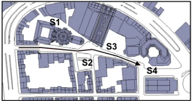
location. In order to study it, we will test them along a route in a model of rue Xavier-Neujean in Liège, represented in figure 2. This route has four interesting sections: S1 is a church, S2 is a place, S3 is an open parking lot, and S4 is crossroads behind a theater. A projection of the sky is calculated every 5 meters on a route of 245 meters.
Figure 2: The route in rue Xavier-Neujean in Liège. We now describe these two measures (GMD radius and GMD location) and present a way to combine them in order to characterize visual sequences of an urban route.
S1
S2 S3
4.1 Greatest maximal disk radius
The radius of the GMD provides results comparable to Teller's open space indicators [20]. This kind of indicator estimates the sense of openness that an observer may feel in an urban space. Figure 3 represents the variation of the GMD radius measure along the route in figure 2. The x-axis represents the image number (position in the path) while the y-axis gives the percentage of GMD radius divided by the radius of the projection circle (maximal value of
GMD).
It can be seen from the graph that the variation of
GMD radius along the route is characterized by four
peaks: position 11, around position 28, position 37, and at the end of the route. Except for the first peak, the others correspond to the sudden appearance of S2, S3, and S4 openings. The first peak in the graph corresponds to the visual opening characterizing points located between the start of the route and the bell tower of the church (S1). Minimums of the curve are also important. The first one is a transition between the space before the church and the place (S2). The next one is due to a narrow part between the place and the parking lot (S3). The last one is a long narrow crossing between S3 and S4.
20 25 30 35 40 45 50 1 6 11 16 21 26 31 36 41 46
Figure 3: GMD radius variation along the route in figure 2.
The GMD radius measure is not tied with the direction of the observer movement. But it detects local openings in the visual environment of the observer. Its variations highlight spaces with a high openness and transitions between these spaces.
4.2 Relative GMD location
Along a route, the location of the GMD varies around the center of the spherical projection: the GMD can be located in the front or in the back of the observer, with respect to his direction. By this way, it is possible to determine at which time an observer perceives the most important local opening.
Figure 4 shows the rear-front location measure of the GMD, in the environment represented in figure 2. It is computed according to the center of the projection and the observer orientation in the route. When the value is superior to 0, the observer sees the
GMD, otherwise it is in his back.
-60 -40 -20 0 20 40 60 1 6 11 16 21 26 31 36 41 46
Figure 4: GMD rear-front location graphics for the route in figure 2.
From the graph of figure 4, we can notice the four series of peaks. These are due to the appearance of the four openings described in the preceding section. For example, between positions 19 and 26, the observer can see an opening on his front before his entrance in place (S2). The entrance starts at the image 22. After image 26, the observer is still in the place but his visual field contains the narrow part between the place and the parking lot. This narrow part is a transition.
The rear-front GMD location provides a mean to situate the local opening from a given location. In the route context, it highlights interesting visual events which are the appearance and disappearance of openings in the stream of urban shape variation. Hence, this measure is relative to the observer direction and it benefits of the same stability than the
GMD radius measure. Moreover, it highlights
openings in front of the observer.
4.3 Combination between the GMD radius and the GMD location
The GMD location describes a partition of the route into parts where GMD is in front of the observer and transition parts. The GMD radius provides information about the importance of the GMD. The combination of these two measures brings a rich interpretation of the selected route.
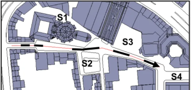
Figure 5 represents the route partition according to the graph in figure 4. It highlights the part of the route (with lines in bold), where the GMD is in the visual field of the observer.
Figure 5: The route partition in rue Xavier-Neujean with respect to the figure 4.
S2 S1
S3
The part of the route which is highlighted in the place (S2) is one of the most important. According to figure 3, it is characterized by a wide opening that the observer sees on his right during a long time. This place appears suddenly. Just before, for approximately the same time, the observer perceives a narrowing between the church (S1) on his left and the building on his right. After in the place, the observer begins to see another narrowing before to arrive near the parking lot (S3). The effect between S2 and S3 is interesting. Indeed there is a kind of competition between these two openings. Finally, according to the graphs 3 and 4, the opening in S4 is seen directly in the visual field of the observer and grows gradually till the end of the route.
With the help of the GMD radius, the GMD rear-front location measure enables to partition a given route into sequences, with respect to the potential interest of the observer.
5 Conclusion
A new method to analyze urban open spaces has been introduced and discussed in this paper. It is based on the study of the sky shape variations in the visual field of the observer along a route. This method uses spherical projections and skeletonization, which brings a new approach to analyze the motion-perspective.
The measures associated with this method are based on the extraction of the GMD, which is the skeletal point with the higher distance from the boundary. The GMD radius is relevant to the visual environment of the observer. Whereas, the GMD rear-front location is relevant to the observer direction along a route. The combination of these two measures allows to partition urban routes into sequences, with respect to the potential interest of the observer.
The method presented here is dedicated to the characterization of dense urban spaces. It gives a dynamic assessment of urban visual quality, and can help to enhance existing tools which analyze the urban environment location by location. Nevertheless, tests and improvements of the measures will certainly be required in order to have a better precision and interpretation of the method.
6 References
[1] D. Appleyard, K. Lynch, and J. R. Myer. The view from the road. MIT Press, 1966.
[2] M. L. Benedikt. To take hold of space: isovists and isovist fields. Environment and Planning B, 6:47-65, 1979. [3] H. Blum. A transformation for extracting new descriptors of shape. In W. Wathen-Dunn, editor, Proceedings of Models for the Perception of Speech and Visual Form, pages 362-380. MIT Press, 1967.
[4] G. Borgefors. Distance transformations in arbitrary dimensions. Computer Vision, Graphics and Image Processing, 27:321-345, 1984.
[5] P. Bosselman. Representation of places: reality and realism in city design. University of California Press, 1998. [6] S. W. Choi and H.-P. Seidel. One-sided stability of medial axis transform. In S. F. E. Bernd Radig, editor, Proceedings of Pattern Recognition, 23rd DAGM Symposium, volume LNCS 2191, pages 132-139, Munich, Germany, 2001.
[7] G. Cullen. The concise townscape. Butterworth Architecture, 1961.
[8] P. Dimitrov, C. Pillips, and K. Siddiqi. Robust and efficient skeletal graphs. In Proceeding of Conference on Computer Vision and Pattern Recognition (CVPR), pages 417-423, Hilton Head, South Carolina, 2000.
[9] F. Fol-Leymarie. Three-dimensional shape representation via shock flows. PhD thesis, Brown University, Providence, Rhode Island, USA, May 2003. [10] J. J. Gibson. The Perception of the Visual World. The River-side Press, Cambridge, Massachusetts, 1950. [11] B. Hillier and J. Hanson. The social logic of space. Cambridge University Press, 1984.
[12] S. Loncaric. A survey of shape analysis techniques. Pattern Recognition, 31(8):983-1001, 1998.
[13] K. Lynch. The image of the city. MIT Press, 1960. [14] R. L. Ogniewicz and O. Kübler. Hierarchic Voronoi skeletons. Pattern Recognition, 28(3):343-359, 1995. [15] J. Peponis, J. Wineman, M. Raschid, S. H. Kim, and S. Bafna. On the description of shape and spatial configuration inside buildings: convex partitions and their local properties. Environment and Planning B: Planning and Design, 24(5):761-781, 1997.
[16] G. Sanniti di Baja and E. Thiel. Skeletonization algorithm running on path-based distance maps. Image and Vision Computing, 14(1):47-57, 1996.
[17] F. Sarradin, D. Siret, and G. Hégron. Visual analysis of urban environment. In Proceedings of First International Workshop on Architectural and Urban Ambient Environment, Nantes, France, February 2002. [CDROM]. [18] K. Siddiqi, S. Bouix, A. Tannenbaum, and S. W. Zucker. Hamilton-jacobi skeletons. International Journal of Computer Vision, 48(3):215-231, 2002.
[19] J. Teller. La régulation morphologique dans le cadre du projet urbain : spécification d'instruments informatiques destinés à supporter les modes de régulation performantiels. Thèse de doctorat, Université de Liège, 2001.
[20] J. Teller. A spherical metric for the field-oriented analysis of complex urban open spaces. Environment and Planning B: Planning and Design, 30:339–356, 2003. [21] P. Thiel. La notation de l'espace, du mouvement et de l'orientation. Architecture d'Aujourd’hui, 145:49-58, 1969. [22] A. Turner, M. Doxa, D. O'Sullivan, and A. Penn. From isovists to visibility graphs: a methodology for the analysis of architectural space. Environment and Planning B,28(1):103-121, 2001.