HAL Id: hal-01756732
https://hal.archives-ouvertes.fr/hal-01756732
Preprint submitted on 2 Apr 2018
HAL is a multi-disciplinary open access archive for the deposit and dissemination of sci-entific research documents, whether they are pub-lished or not. The documents may come from teaching and research institutions in France or abroad, or from public or private research centers.
L’archive ouverte pluridisciplinaire HAL, est destinée au dépôt et à la diffusion de documents scientifiques de niveau recherche, publiés ou non, émanant des établissements d’enseignement et de recherche français ou étrangers, des laboratoires publics ou privés.
The nexus between FDI and environmental
sustainability in North Africa
Marwa Lazreg, Ezzeddine Zouari
To cite this version:
Marwa Lazreg, Ezzeddine Zouari. The nexus between FDI and environmental sustainability in North Africa. 2018. �hal-01756732�
1
The nexus between FDI and environmental sustainability in North Africa
Marwa Lazregh *
Faculty of Economic and Management Sciences of Sousse University of Sousse, Tunisia
E-mail: [email protected]
* Corresponding author
Ezzeddine Zouari
Faculty of Economic and Management Sciences of Sousse University of Sousse, Tunisia
E-mail: [email protected]
Abstract: This paper provides a study of the relationship between sustainable development
and foreign direct investment (FDI) from an empirical point of view in the case of the North African country during the period from 1985 to 2005. We used the FMOLS estimate and the causality test to examine this relationship. According to the results found, we confirmed the existence of a cointegration relationship between the different series studied in this paper. Indeed, the results of the null hypothesis test of no cointegration were rejected at the 5% threshold, which explains the presence of a cointegration relationship. The cointegration test can determine the use of a model error correction. Also, to test the effect of FDI on sustainable development in the countries of North Africa, we will make an estimate by FMOLS method. We found that the LIDE variable measuring foreign direct investment has a positive impact on sustainable development. Also, we notice that there is a bidirectional relationship between FDI and emissions CO2 Granger. That is to say, the IDE can cause Granger emissions of CO2 and CO2 emissions can cause Granger FDI.
Keywords: foreign direct investment; sustainable development; CO2; Poverty, panel data Biographical notes: Dr. Marwa Lazreg is a PhD in Economics at the Faculty of Economic
Sciences and Management of Sousse, Tunisia. His research interests include Economic analysis, financial economics, quantitative finance, financial development, and energy commodities. He is one of the Editorial Board Members in the International Journal of Management and Enterprise Development.
Dr. Ezzeddine Zouari is a Professor in Finance at the Higher Institute of Management of Sousse in University of Sousse, Tunisia. His research interests include Capital markets and institutions, Banking and market microstructure, financial economics, quantitative finance, financial development and Islamic Finance.
2
1. Introduction
Regarding the relationship between FDI and the environment, a lot of literature also focuses on their potential link. For example, Hoffmann et al. (2005) use the Granger causality test based on data from 112 countries to ensure that the relationship between FDI and pollution depends on the development of the host countries.
Cole et al. (2006) develop a model of political economy and concluded that when the degree of corruptibility of the government is weak, FDI leads to a stricter and cleaner environmental policy.
Hitam and Borhan (2012) use data of Malaysia from 1965 to 2010 to examine the impact of FDI on the quality of the environment and concluded that FDI would increase environmental pollution. Therefore, FDI should be incorporated as an independent variable in the regression model CEK, otherwise, the estimated coefficients from the regression equation CEK will be biased because of omitted variable.
Grossman and Krueger (1995) establish a relationship between economic growth and environmental pollution. Their conclusion shows that environmental pollution and per capita income exist inverted U shape, which is popular as environmental Kuznets curve (EKC), the quality of the environment does not deteriorate with both economic growths beyond the turning point.
According to the study by Grossman and Krueger (1995), some studies (Selden and Song, 1995; Jones and Manuelli, 2001; Hartman and Kwon, 2005; Brock and Taylor, 2010) Construct various theoretical models (eg model of overlapping generations) to find the possible reasons for the inverted U-shape between economic growth and economic pollution. In these models, they assume that individual utility is a function of the normal quality of goods and the environment, resulting in a compromise between the normal property and environmental quality to maximize the utility level when resource constraints are imposed. A significant difference between these theoretical models is that they offer different mechanisms to explain the existence of an inverted U-shaped pattern. For example, Stocky (1998) point out that the choice of optimal production technology in different periods of development resulted in the CEK.
Jones and Manuelli (2001) change the outlook from technology to political factors, they showed that the pollution tax and / or regulations may interpret the formation of the CEK. For most of the existing literature, they neglect one important feature that the impact of FDI on environmental pollution depends on the level of economic development, in other words, the effect of FDI on environmental quality varies according to the development period. The pollution is based on GDP and should be considered as a function of GDP.
In addition, most empirical research using the quadratic term and the cubic term to capture the nonlinear effect of GDP and / or FDI on the environment, prior specification of the regression function may bias the results as mentioned by Harbaugh et al. (2002).
This paper provides a study on sustainable development and foreign direct investment (FDI) from an empirical point of view in the case of the North African country during the period from 1985 to 2005.
3
Then, we use the estimation FMOLS and causality test. According to the results found, we confirmed the existence of a cointegration relationship between the different series studied in this paper. Indeed, the results of the null hypothesis test of no cointegration were rejected at the 5% threshold, which explains the presence of a cointegration relationship. The cointegration test can determine the use of a model error correction. Also, to test the effect of FDI on sustainable development in the countries of North Africa, we will make an estimate by FMOLS method. We found that the LIDE variable measuring foreign direct investment has a positive impact on sustainable development. Also, we noticed that there is a bidirectional relationship between FDI and emissions CO2 Granger (0.0000 < 5% and 0.0000 < 5%). That is to say, the IDE can cause Granger emissions of CO2 and CO2 emissions can cause Granger FDI.
The rest of the paper is organized as follows: In Section 2, we present a literature review. The third section summarizes the econometric methodology. Data are presented in Section 4. Section 5 was dedicated to the interpretation of results. The conclusion is made in section 6.
2. Literature review
Moreover, Borenszteina et al. (1998) study the impact of foreign direct investment (FDI) on economic growth in developing countries through panel data for 69 countries for two decades from 1970 to 1989 .The authors have regression estimation oN using the technique, the results showed that FDI is an important vehicle for technology transfer, contributing to growth relatively more than domestic investment. However, the greater productivity of FDI holds only when the host country has a minimum threshold stock of human capital. Thus, FDI contributes to economic growth only if sufficient capacity to absorb advanced technologies available in the host economy.
Similarly, Nair-Reichert and Weinhold (2001) analyze the effect of FDI on growth with a panel of 24 developing countries over 25 years using a mixed approach of fixed and random coefficient (mixed fixed and random coefficient approach) this study explored that The FDI has averaged a significant positive impact on growth, but the relationship is heterogeneous across countries.
Besides, Manuchehr and Ericsson (2001) work on the causality between foreign direct investment and production based on a sample of four countries Denmark, Finland, Sweden and Norway for the period 1970-1997. They have used Lag-augmented vector autoregression method that shows causal bi suede and FDI has a positive effect on economic growth in the country of Norway.
The study Choe (2003) tried to show the causal relationship between economic growth and FDI and GDP in 80 countries during the period 1971-1995, using the Granger causality test results show that FDI Granger because I economic growth and vice versa;
In addition to Article Chowdhury and Mavrotas (2006) examine the causal relationship between FDI and economic growth using innovative econometric methodology to study the direction of causality between the two variables. They applied their methodology, based on Lag-augmented vector autoregression with time-series data covering the period 1969-2000 for three developing countries, namely Chile, Malaysia and Thailand, their empirical results showed that there is strong evidence of a bidirectional causality between the two variables for Malaysia and Thailand.
4
In addition, Chakraborty and Nunnenkamp (2006) analyze the effect of FDI on India's economy; the authors took a 1987-2000 period by applying the model Granger causality test. They found bidirectional causality in the industry sector manufacturing. While FDI has a positive effect on economic growth.
The study of Al-Iriani (2007) also examines the association between foreign direct investment and economic growth. The sample consists of six countries including the Gulf Cooperation Council (GCC). For a period of 1970-2004. The model used is Granger causality test of Holtz-Eakin. The results of an analysis panel heterogeneous indicate bidirectional causality between FDI and GDP in this group of GCC countries. Hence the FDI has a positive effect on economic growth
Regarding research Shaikh (2010) who has studied the causal link between FDI and economic growth of trade in Pakistan using time series of quarterly data from 1998 to 2009, the model OLS showed bidirectional causality between foreign direct investment and economic growth, and foreign direct investment has a positive impact on the growth of trade in Pakistan and especially in the manufacturing sector. Moreover Shaikh applied the same methodology in Malaysia for a further period from 1970 to 2005 to confirm the significant positive relationship between these two variables.
Davletshin et al. (2015) were the analysis of the relationship between the flow of foreign investment in the country and economic growth by taking two groups: developed country group and group of developing countries, the analysis is based on the correlation test for period 1995-2012, the results show that GDP depends directly on IDF and the IDF effect on GDP is strong and important in developing countries.
Moreover, Iamsiraroj (2016) studies the relationship between FDI and economic growth through panel data from 124 countries covering the period from 1971 to 2010. In estimating the author used the method of OLS. The estimation results indicate that the overall effects of FDI are positively associated with growth and vice versa, so there is a bidirectional relationship between FDI and economic growth.
Still, the study of Pegkas (2015) including its goal is twofold: first; analyze the relationship between foreign direct investment and economic growth, and second; Estimate the effect of FDI on economic growth using panel data for countries in the euro area over the period from 2002 to 2012 and applying the method of OLS completely changed (FMOLS) and dynamic OLS (DOLS). The empirical analysis revealed that there is a lasting positive co-integration relationship between the stock of FDI and economic growth, and the results show that the stock of foreign direct investment is a significant factor that positively affects growth economic pays.de of Europe.
3. Empirical Methodology
This paper provides a study on sustainable development and foreign direct investment (FDI) from an empirical point of view in the case of the North African country during the period from 1985 to 2005.
5 0 1 2 3 4 5 6 7 8 9 10 11 12 13 14 15 16 2 1.91$ 3.1$ it it it it it it it it it it it it it it it it it it
LCO LIDE LGINI LINF LPIB LPU
LTAJ LUE LIDE LDEP LDEF LFBC
LCH LCER LCBEC LPOV LPOV
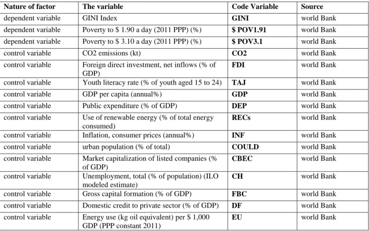
Or, 0is a constant, iare coefficients of the explanatory variables i = 1, ..., 16, t = 1, ..., 31 and it it is the term of error. Table 1 summarizes the different variables used in our paper.
Table 1: The different variables
Nature of factor The variable Code Variable Source
dependent variable GINI Index GINI world Bank
dependent variable Poverty to $ 1.90 a day (2011 PPP) (%) $ POV1.91 world Bank
dependent variable Poverty to $ 3.10 a day (2011 PPP) (%) $ POV3.1 world Bank
control variable CO2 emissions (kt) CO2 world Bank
control variable Foreign direct investment, net inflows (% of GDP)
FDI world Bank
control variable Youth literacy rate (% of youth aged 15 to 24) TAJ world Bank
control variable GDP per capita (annual%) GDP world Bank
control variable Public expenditure (% of GDP) DEP world Bank
control variable Use of renewable energy (% of total energy consumed)
RECs world Bank
control variable Inflation, consumer prices (annual%) INF world Bank
control variable urban population (% of total) COULD world Bank
control variable Market capitalization of listed companies (% of GDP)
CBEC world Bank
control variable Unemployment, total (% of population) (ILO modeled estimate)
CH world Bank
control variable Gross capital formation (% of GDP) FBC world Bank
control variable Domestic credit to private sector (% of GDP) DF world Bank
control variable Energy use (kg oil equivalent) per $ 1,000 GDP (PPP constant 2011)
EU world Bank
The data used in this paper are of annual frequency for all variables. These data come from the World Bank database and the International Monetary Fund for the period from 1985 to 2015.We will estimate the models chosen by referring to an analysis of panel data.
The choice of panel data is based on the two dimensions of the data used; the first dimension is time (a period of 31 years) and the second is individual (employee sample consists of 6 countries of North Africa).
4. Data
In this section, we present the sample and the model used in our paper.
Our objective in this paper, Is the study of the impact of FDI on poverty in the case of the North African country during the study period between 1985 and 2015.
In Table 2, we exposed the different countries in ourpaper.
Table 2: The countries of North Africa
Name countries Area (km) Population (2016 estimate) Population density (per km²)
6 Egypt 1001450 81,249,302 80.4 Libya 1759540 6461450 3.7 Morocco 710 850 32,245,000 70.8 Sudan 1886068 31957965 16.9 Tunisia 163610 10673000 64.7
In this section we will try to make a descriptive analysis of the different results for the study the impact of FDI on poverty in the countries of North Africa.
First, let's define the type of assessment which is a regression on panel data. Our choice is justified by the presence of two dimensions in the data used; is the first time (a period of 31 years) and the second is individual (our sample is made up of 6 countries of North Africa). This section is dedicated to the interpretation of results for the descriptive statistics and Pearson correlation matrix for the variables used in our paper.
All of the descriptive statistics of the variables used in our paper are summarized in Table 3. According to the results of Table 3, we found that the LCO2 variable, which expresses logarithm of CO2 emissions, can reach a maximum value of 12.30497. As its minimum value is 7.975197. Its risk is measured the standard deviation is 1.022934.
The LGINI variable, which measures the logarithm of the GINI index, can reach a maximum value of 4.146937. While its minimum value is 3.425890. Its risk is measured the standard deviation is 0.192268.
The variable $ LPOV1_91, which measures the logarithm of the gap of poverty threshold of $ 1.91 may reach a maximum value of 3.801985. As its minimum value is -0.916291. Its risk is measured by the standard deviation is 1.537783.
The variable $ LPOV3_1, which measures the logarithm of the poverty gap at $ 3.1 threshold, can reach a maximum value of 4.074482. As its minimum value is 0.741937. Its risk is measured the standard deviation is 1.007091.
Both statistics of asymmetry (skewness) and kurtosis (kurtosis), we can conclude that all variables used in this paper are characterized by non-normal distribution. Then the asymmetry coefficients indicate that all variables are shifted to the left (negative sign of asymmetry coefficients) and is far from symmetrical except for LGINI variables, LIDE, LINF, LPIB, READ, LFBC, LCH, LCER LCBEC and which are oriented to the right (positive sign of asymmetry coefficients).
Also, the kurtosis coefficient shows that leptokurtic for all variables used in this paper indicate the presence of a high peak or a large tail in their volatilities (leptokurtic the coefficients are greater than 1).
In addition, the positive sign of estimation coefficients of Jarque-Bera statistics indicates that we can reject the null hypothesis of the normal distribution of the variables used in our paper. In fact, the high value of the coefficients of the Jarque-Bera statistic reflects the series are not normally distributed at a level of 1 percent.
The results shown by the three skew statistics, kurtosis and Jarque-Bera suggest that all variables used in our paper are not normally distributed for the case of the countries of North Africa and during the study period from 1985 to 2015.
Thus, we conducted a test of the correlation between the different variables used in the case of the North African country during the study period from 1985 to 2015. Table 4 summarizes the results for test Pearson correlation.
7
In addition, the results showed that all coefficients between the explanatory variables do not exceed the tolerance limit (0.7), what does not cause problems in the estimation of the model. That is to say, we can integrate the different variables used in the same model.
A study of the causal relationship between FDI and poverty in the countries of North Africa requires prior perform stationary tests to determine the order of integration of each series. The results of the Levin-Lin-Chu test (LLC), Im-Pesaran-Shin (IPS), ADF and Fisher-PP-Fisher applied to the series are shown in Table 5 for country of North Africa.
Acceptance or rejection of the null hypothesis of the different tests is based on the value of probability and the indicated test statistics. These probabilities are compared with a 10% threshold. If these probabilities are less than 10%, then we reject the null hypothesis and if these probabilities are greater than 10%, then we accept the null hypothesis.
For the countries of North Africa and in Table 5, we observed that only two variables LIDE, LPIB and LUE are non-stationary in level according to the test of Levin-Lin-Chu but all variables are stationary in difference first according to this test.
According to statistics of the test-Im Pesaran-Shin (IPS), ADF-Fisher test and the test PP-Fisher, we can conclude that only four variables, LIDE, LPIB, LINF and LUE are stationary in level. But first difference, all variables are stationary according to these three tests. Thereafter, all the variables are integrated of order 1. Thus, we can use the cointegration test.
8 Table 3: Descriptive statistics
LGINI $ LPOV1_91
$ LPOV3_1 LCO2 LIDE LINF LPIB LPU
Average 3.659430 1.711339 2.819903 10.52246 1.740903 12.13125 1.966823 3.953845 Median 3.572328 1.751173 2.913658 10.57184 1.226897 5.737290 1.894978 4.005441 Maximum 4.146937 3.801985 4.074482 12.30497 9.424248 132.8238 104.6576 4.361301 Minimum 3.425890 -0.916291 0.741937 7.975197 -0.469340 -9.797647 -62.21435 3.132751 Standard Deviation 0.192268 1.537783 1.007091 1.022934 1.875266 21.34465 9.915128 0.299145 skewness 1.017615 -0.314673 -0.407684 -0.437984 1.658814 3.792586 4.340137 -0.572764 kurtosis 3.330697 1.869836 1.860567 2.615518 6.371119 18.51450 72.66292 2.511294 Jarque-Bera 32.94928 * 12.96843 * 15.21429 * 7.092390 * 173.3760 * 2311.317 * 38194.09 * 12.02076 * Probability 0.000000 0.001527 0.000497 0.028834 0.000000 0.000000 0.000000 0.002453 Sum 680.6540 318.3091 524.5020 1957.178 323.8080 2256.413 365.8290 735.4151 Sum Sq. Dev. 6.838913 437.4836 187.6328 193.5830 650.5753 84284.89 18187.31 16.55519 observations 186 186 186 186 186 186 186 186
LTAJ LUE LDEP LDF LFBC CHL LCER LCBEC
Average 4.397266 4.647219 2.760326 3.117432 24.17608 2.671726 1.880000 3.329833 Median 4.400727 4.538225 3.187676 3.306042 24.53558 2.694627 2.356580 3.180049 Maximum 4.604464 5.460651 3.566570 4.336893 46.87646 3.394508 4.450014 5.622575 Minimum 4.067913 4.276705 1.401579 0.479664 4.329239 2.091864 -1.730354 0.716136 Standard Deviation 0.148325 0.288363 0.742070 0.959663 7.523842 0.292898 1.737291 1.399367 skewness -0.428835 1.298344 -0.776126 -0.727663 0.207327 0.045106 -0.529717 -0.324575 kurtosis 2.526260 3.880495 1.924430 2.732941 3.446433 2.417982 2.494614 2.045393 Jarque-Bera 7.440210 ** 58.26498 * 27.63912 * 16.96701 * 200.877117 232.688345 10.67806 * 10.32820 * Probability 0.024231 0.000000 0.000001 0.000207 0.000000 0.000000 0.004801 0.005718 Sum 817.8915 864.3827 513.4206 579.8423 4496.752 496.9410 349.6800 619.3490 Sum Sq. Dev. 4.070076 15.38337 101.8735 170.3764 10472.52 15.87098 558.3630 362.2723 observations 186 186 186 186 186 186 186 186
9 Table 4: The correlation matrix
LGINI $ LPOV1_91
$ LPOV3_1 LCO2 LIDE LINF LPIB LPU
LGINI 1.000000 0.216744 0.154968 -0.165647 -0.220977 -0.227902 -0.017152 0.653434 $ LPOV1_91 0.216744 1.000000 0.089412 0.399300 -0.211419 0.025710 -0.059185 0.176666 $ LPOV3_1 0.154968 0.089412 1.000000 0.457670 -0.226173 0.013915 -0.057560 0.144844 LCO2 -0.165647 0.399300 0.457670 1.000000 0.000554 -0.472189 -0.028778 0.416057 LIDE -0.220977 -0.211419 -0.226173 0.000554 1.000000 -0.175203 0.107440 -0.116444 LINF -0.227902 0.025710 0.013915 -0.472189 -0.175203 1.000000 -0.034212 -0.550643 LPIB -0.017152 -0.059185 -0.057560 -0.028778 0.107440 -0.034212 1.000000 -0.022537 LPU 0.653434 0.176666 0.144844 0.416057 -0.116444 -0.550643 -0.022537 1.000000 LTAJ 0.526538 0.287783 0.208722 0.066702 0.093524 -0.139248 -0.014518 0.535036 LUE 0.274596 0.255015 0.194614 -0.655195 -0.074166 0.565342 -0.090298 -0.340264 LDEP -0.622753 -0.437272 -0.386163 0.404099 0.115025 -0.256776 -0.007249 0.011678 LDF 0.057127 -0.258985 -0.274410 0.330278 0.061514 -0.508943 -0.049271 0.390001 LFBC -0.167209 -0.192547 -0.163840 0.278071 0.174104 -0.297027 -0.008009 0.278378 CHL 0.478501 0.349806 0.310655 -0.192702 -0.311803 0.043348 -0.046815 0.281923 LCER -0.160403 -0.551713 -0.579122 -0.017235 0.273491 0.341804 0.070820 -0.627556 LCBEC -0.467603 -0.061890 0.025036 0.622213 -0.079906 -0.251845 -0.017867 0.102219
LTAJ LUE LDEP LDF LFBC CHL LCER LCBEC
GINI 0.526538 0.274596 -0.622753 0.057127 -0.167209 0.478501 -0.160403 -0.467603 $ POV1_91 0.287783 0.255015 -0.437272 -0.258985 -0.192547 0.349806 -0.551713 -0.061890 $ POV3_1 0.208722 0.194614 -0.386163 -0.274410 -0.163840 0.310655 -0.579122 0.025036 CO2 0.066702 -0.655195 0.404099 0.330278 0.278071 -0.192702 -0.017235 0.622213 FDI 0.093524 -0.074166 0.115025 0.061514 0.174104 -0.311803 0.273491 -0.079906 INF -0.139248 0.565342 -0.256776 -0.508943 -0.297027 0.043348 0.341804 -0.251845 GDP -0.014518 -0.090298 -0.007249 -0.049271 -0.008009 -0.046815 0.070820 -0.017867 COULD 0.535036 -0.340264 0.011678 0.390001 0.278378 0.281923 -0.627556 0.102219 TAJ 1.000000 0.287557 -0.393472 0.034387 -0.101385 0.309117 -0.278047 -0.444202 EU 0.287557 1.000000 -0.038724 -0.542902 -0.515000 0.271294 0.379276 -0.029952 DEP -0.393472 -0.038724 1.000000 0.538695 0.485806 -0.438228 -0.139890 0.011836 DF 0.034387 -0.542902 0.538695 1.000000 0.167907 -0.338843 -0.085541 0.181762 FBC -0.101385 -0.515000 0.485806 0.167907 1.000000 -0.180540 -0.400536 0.556466 CH 0.309117 0.271294 -0.438228 -0.338843 -0.180540 1.000000 -0.331089 -0.283439 RECs -0.278047 0.379276 -0.139890 -0.085541 -0.400536 -0.331089 1.000000 -0.489024 CBEC -0.444202 -0.029952 0.011836 0.181762 0.556466 -0.283439 -0.489024 1.000000
10 Table 5: The unit root test
Levin, Lin and Chu test Im Pesaran and Shin test Fisher-ADF test Fisher-PP test
in level In the first difference
in level In the first difference
in level In the first difference
in level In the first difference LGINI 0.04843 -8.49929 * 0.89018 -8.20229 * 2.29937 * 60.0539 2.40167 * 55.2620 $ LPOV1_91 -0.14884 -5.74166 * 1.42407 -4.50321 * 3.24554 * 30.8073 3.11444 * 62.9879 $ LPOV3_1 0.16586 -6.66453 * 1.83580 -5.19057 * 2.70321 * 40.9005 2.59457 * 75.6234 LCO2 -2.31532 ** -4.30995 * 0.69587 -7.07982 * 8.56954 * 69.5309 9.67859 154 030 * LIDE -1.34558 *** -7.74929 * -1.45050 *** -7.72450 * 17.4511 * 77.2053 21.3662 ** 110 975 * LINF -0.95540 -4.66477 * -1.15735 -8.10519 * 15.8569 * 80.9894 19.9673 *** 169 770 * LPIB -1.51908 *** -8.99655 * -6.75610 * -15.2398 * * 69.8560 143 243 * 114 075 * 147 112 * LPU 0.27789 -3.04947 * 1.41163 -2.65498 * 8.52763 * 38.9532 5.71631 * 96.0690 LTAJ 0.92601 -6.17024 * 2.71270 -5.34750 * 1.70601 * 42.3096 1.56592 * 82.1910 LUE 0.94164 -6.57636 * 0.52071 -7.52213 * 11.7411 * 74.3314 20.9092 *** 166 572 * LDEP 0.10824 -4.94802 * 0.78000 -4.79169 * 6.71074 * 37.6871 6.01183 * 74.3079 LDF -0.45709 -2.94146 * 0.07851 -4.68708 * 8.62522 * 47.3625 8.09243 * 87.9162 LFBC -0.55114 -8.91245 * -0.27310 -8.55507 * 12.4720 * 86.1683 12.9794 109 564 * CHL 1.16977 -8.14926 * 0.72209 -3.48922 * 6.58552 * 36.7939 9.46106 104 902 * LCER 0.35985 -6.81112 * 1.81424 -7.27592 * 4.81480 * 73.3678 4.84895 145 911 * LCBEC 1.40710 -4.90207 * 0.84712 -6.38119 * 8.13605 * 62.8924 12.1554 118 134 *
Note: In this test, the p-value is compared to 10%. If the probabilities <10% therefore we reject the null hypothesis and the
probabilities> 10% then we accept the null hypothesis. With the null hypothesis all series are non-stationary. (*), (**) and (***) are significant values for the 1% and 5% respectively.
5. Empirical Analysis
5.1. The cointégrattion test
We will expose in this part of the test results of cointegration. Kao tests, Pedroni and Johenson Fisher cointegration are used to verify the long-term relationship between the variables used in this paper to examine the impact of pollution on IDEs (sustainable development) in the case of countries North Africa.
11
The Kao test is based on the statistical t-test and ADF Pedroni is based on two statistical Panel and Panel-ADF-PP individual and grouped. But Fisher's test is based on the Fisher statistical test track and Fisher Statistic of max-eigen test. The results of cointegration test for the countries of North Africa are presented in Table 6.
Indeed, the Pedroni test demonstrates the long-term relationship between the IDEs and sustainable development. Thus, Kao test confirms the long-term relationship between the different variables used in this paper, mainly between IDEs and sustainable development.
In addition, Fisher's test results confirm the presence of a long-term relationship between IDEs and sustainable development in the countries of North Africa for the study period from 1985 to 2015.
According to the results in Table 6, we have confirmed the existence of a cointegration relationship between the different series studied in this paper. Indeed, the results of the null hypothesis test of no cointegration were rejected at the 5% threshold, which explains the presence of a cointegration relationship.
The results of these tests can determine the use of an error correction model. Also, to test the effect of FDI on sustainable development in the countries of North Africa, we will perform a FMOLS estimate.
Table 6: The cointegration test of the impact of FDI on sustainable development for countries of North Africa
Pedroni Residual Cointegration Test Kao Residual
Cointegration Test
Fisher Johansen Cointegration Test Panel
Common AR coefs. (Within-dimension)
Individual AR coefs. (Between-dimension) Statistics (Probability) Fisher Stat. * (From test track)
Prob. Fisher Stat. * (From max-eigen test) Prob. PP-Statistic Panel ADF-Statistic Panel -2.817652 (0.0024) * -4.053302 (0.0000) * PP-Statistic Panel ADF-Statistic Panel -2.677227 (0.0037) * -4.637353 (0.0000) * -4.010569 (0.0000) * 199.5 (0.0000) * 112.6 (0.0000) *
13 5.2. The error correction model (ERM)
After testing the cointegration between FDI and sustainable development in our paper, we'll estimate the model for correction of errors.
The MCE allows modeled together for short-term dynamics (represented by the variables in first differences) and long term (represented by the variables in level).
Table 7 summarizes the estimated error correction model for sustainable development and for the countries of North Africa during the study period of 1985 to 2015.
For LIDE variable and studying the short-term dynamics, we noticed that the IDE (t-2) have a positive and significant impact on a threshold of 1% of foreign direct investment at time t for the case North African countries. That is to say, if the IDE at the time (t-2) increased by one then, foreign direct investment increased by 0.265404 units.
Poverty measured by the GINI index has a negative and significant impact on foreign direct investment at a 10% threshold. That is to say, if the GINI index of 10 units, then, foreign direct investment fell by 3.518615 units.
The LINF variable that measures the consumer price index also has a negative and significant impact on foreign direct investment with a threshold of 5%. That is to say, if the level of the inflation rate increases by five units, then, foreign direct investment fell by 0.016970 units. The LUE variable that measures the level of energy consumption is statistically significant and positive impact on foreign direct investment to a level of 5%. So if energy consumption increases five units then, foreign direct investment increased by 1.659182 units.
The LFBC variable that measures the gross formation of capital stock also has a positive and significant impact on foreign direct investment with a threshold of 1%. That is to say, if the level of gross fixed capital stock increases by one, while foreign direct investment increased by 0.059556 units.
The LCER variable that measures the consumption of renewable energy has a positive and significant impact on foreign direct investment with a threshold of 1%. That is to say, if the level of consumption of renewable energy increased by one, while foreign direct investment increased by 0.619481 units.
For sustainable development, we note that emissions of CO2 at the time (t-1) have a negative and significant effect on CO2 emissions at t a% threshold. This means that if emissions of CO2 at the time (t-1) increase by one when they fell by 0.401891 units at time t.
The LINF variable that measures the consumer price index also has a negative and significant impact on emissions of CO2 at a threshold of 5%. That is to say, if the level of the inflation rate increases by one, then the CO2 emissions decrease to 0.001444 units.
The LCBEC variable that measures the market capitalization of listed companies is statistically significant and positive CO2 emissions to a 10% threshold. So if the market capitalization of listed companies increased by ten units then the CO2 emissions increase of 0.026446 units.
14 Table 7: The MCE for variable LCO2
Cointegrating Eq: CointEq1
LIDE (-1) 1.000000
LCO2 (-1) -1.389206
(0.52364) [-2.65299] **
C 12.83399
Error correction: D (LIDE) D (LCO2)
CointEq1 -0.573241 0.010564 (0.08189) (0.00654) [-7.00033] * [1.61631] D (LIDE (-1)) 0.138686 -0.001438 (0.08452) (0.00675) [1.64088] [-0.21316] D (LIDE (-2)) 0.265404 0.002442 (0.07799) (0.00622) [3.40303] * [0.39234] D (LCO2 (-1)) 1.654061 -0.401891 (1.00477) (0.08019) [1.64620] [-5.01151] * D (LCO2 (-2)) 2.396795 -0.067375 (0.96360) (0.07691) [2.48733] [-0.87605] C -7.842108 0.307039 (9.47774) (0.75644) [-0.82742] [0.40590] LGINI -3.518615 0.017769 (1.90225) (0.15182) [-1.84971] *** [0.11703] $ LPOV1_91 0.488675 -0.013726 (0.64651) (0.05160) [0.75587] [-0.26600] $ LPOV3_1 -0.935288 0.007996 (1.02202) (0.08157) [-0.91514] [0.09802] LINF -0.016970 -0.001444 (0.00655) (0.00052) [-2.59077] ** [-2.76299] * LPIB 0.012013 0.000539 (0.00970) (0.00077) [1.23820] [0.69627] LPU 1.234348 -0.110114 (1.26188) (0.10071) [0.97818] [-1.09333] LTAJ 1.478636 -0.027672 (1.23857) (0.09885) [1.19383] [-0.27993] LUE 1.659182 0.066109 (0.81033) (0.06467) [2.04755] ** [1.02218] LDEP -0.357099 -0.025279 (0.48293) (0.03854) [-0.73944] [-0.65584] LDF -0.102722 0.007644 (0.22079) (0.01762) [-0.46525] [0.43379]
15 LFBC 0.059556 -0.002622 (0.02136) (0.00170) [2.78848] * [-1.53825] CHL 0.828491 -0.009341 (0.53879) (0.04300) [1.53769] [-0.21721] LCER 0.619481 -0.007170 (0.21316) (0.01701) [2.90615] * [-0.42146] LCBEC -0.011525 0.026446 (0.17641) (0.01408) [-0.06533] [1.87827] *** R-squared 0.713195 0.759906 Adj. R-squared 0.725025 0.764894
Note: (*), (**) and (***) are significant values for the 1%, 5% and 10% respectively
5.3. The estimation results FMOLS
The panel FMOLS method proposed by Pedroni (1996.2000) solves problems of heterogeneity in the sense that it allows the use of heterogeneous cointegrating vectors. For Maeso-Fernandez et al. (2004), FMOLS estimator takes into account the presence of the constant term and the possible existence of correlation between the error term and differences estimators.
Adjustments are made to this effect on the dependent variable and long-term parameters obtained by estimating the fitted equation. In the case of panel data, the long-term coefficients from the FMOLS art are obtained by the average group of estimators with respect to the sample size (N).
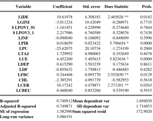
According to Table 8, the coefficient of determination is greater than 0.7, therefore, the estimated model is characterized by a good linear fit.
For FMOLS estimate of the first indicator of poverty, we noticed that there are five significant variables, but with different signs.
We found that the LIDE variable measuring foreign direct investment has a positive impact on sustainable development at a threshold of 5%. That is to say, if the level of foreign direct investment increased by 5 units, while the CO2 emissions increase of 10.61978 units.
Indeed, LPIB which measures the GDP growth rate has a positive and significant impact on sustainable development at a threshold of 1%. This means that if the GDP growth rate increases by one while the CO2 emissions increase of 0.018659 units at time t in the case of the North African country.
The LUE variable which measures the level of energy consumption is statistically significant and positive at a 1% level. So if energy consumption increases by one then the CO2 emissions increase of 4.452260 units.
The LFBC variable that measures the gross formation of capital stock also has a positive and significant impact on sustainable development at a threshold of 5%. That is to say, if the level of gross fixed capital stock increases by five units, while the CO2 emissions increase of 0.244468 units.
16
The LCER variable that measures the consumption of renewable energy has a positive and significant impact on sustainable development at a threshold of 5%. That is to say, if the level of consumption of renewable energy increased by five units, while the CO2 emissions increase of 10.17242 units.
Table 8: Estimation FMOLS for variable LCO2
Variable Coefficient Std. error Does Statistic Prob.
LIDE 10.61978 4.308183 2.465026 ** 0.0162 LGINI -3.011224 10.42049 -0.288971 0.7735 $ LPOV1_91 -1.161451 4.228998 -0.274640 0.7844 $ LPOV3_1 2.217986 6.760589 0.328076 0.7438 LINF -0.090040 0.106092 -0.848699 0.3990 LPIB 0.018659 0.023422 5.796654 * 0.0000 LPU -25.62075 20.10734 -1.274199 0.2069 LTAJ 1.729992 8.980003 0.192649 0.8478 LUE 4.452260 5.405615 5.823636 * 0.0000 LDEP 0.615290 3.503239 0.175634 0.8611 LDF -0.855632 1.758813 -0.486483 0.6282 LFBC 0.244468 0.095770 2.552650 ** 0.0129 CHL -2.385291 4.091739 -0.582953 0.5618 LCER 10.17242 4.478871 2.271201 ** 0.0263 LCBEC 0.460040 0.853206 0.539190 0.5915
R-squared 0.740912 Mean dependent var 1.694030
Adjusted R-squared 0.749871 SD dependent var 1.716853
SE of regression 1.582980 Sum squared resid 172.9020
Long-run variance 5.086191
Note: (*), (**) and (***) are significant values for the 1%, 5% and 10% respectively
5.4. The causality test
We need to check if the IDE cause of CO2 or the CO2 emissions caused FDI in the countries of North Africa.
Acceptance or rejection of the null hypothesis of Granger causality test is based on a threshold of 5%. If the probability of the test is less than 5% in this case we reject the null hypothesis and if the probability is greater than 5% then we accept the null hypothesis of no causality.
Table 9 summarizes the overall results of causality test between FDI and emissions of CO2 for countries of North Africa and the study period of 1985 to 2015.
According to Table 9, we noticed that there is a bidirectional relationship between FDI and emissions CO2 Granger (0.0000 <5% and 0.0000 <5%). That is to say, the IDE can cause Granger emissions of CO2 and CO2 emissions can cause Granger FDI.
Thus, we noticed that there is a unidirectional relationship between sustainable development and economic growth Granger. Only CO2 emissions can cause Granger economic growth. In addition, we noticed that there is a bidirectional relationship between the urban population and emissions CO2 Granger. That is to say, the urban population can cause Granger's CO2 emissions and CO2 emissions can cause Granger urban population.
17 Table 9: The causality test for variable LCO2
Null Hypothesis: Obs F-Statistic Prob.
CO2 does not Granger Cause IDE 174 6.97621 0.0000
FDI does not Granger Cause CO2 7.69724 0.0000
GINI does not Granger Cause CO2 174 2.05242 0.1316
CO2 does not Granger Cause GINI 0.02150 0.9787
$ POV1_91 does not Granger Cause CO2 174 0.41057 0.6639
CO2 does not Granger Cause $ POV1_91 0.29971 0.7414
$ POV3_1 does not Granger Cause CO2 174 0.25712 0.7736
CO2 does not Granger Cause $ POV3_1 0.27003 0.7637
INF does not Granger Cause CO2 174 2.77630 0.0651
CO2 does not Granger Cause INF 1.02793 0.3600
GDP does not Granger Cause CO2 174 1.06934 0.3455
CO2 does not Granger Cause GDP 3.92708 0.0215
PU does not Granger Cause CO2 174 5.41834 0.0052
CO2 does not Granger Cause PU 14.4620 2.E-06
TAJ does not Granger Cause CO2 174 2.27006 0.1064
CO2 does not Granger Cause TAJ 0.95201 0.3880
EU does not Granger Cause CO2 174 1.13016 0.3254
CO2 does not Granger Cause EU 0.19505 0.8230
DEP does not Granger Cause CO2 174 1.31492 0.2712
CO2 does not Granger Cause DEP 0.34891 0.7060
DF does not Granger Cause CO2 174 0.89644 0.4100
CO2 does not Granger Cause DF 2.14380 0.1204
BCF does not Granger Cause CO2 174 0.08322 0.9202
CO2 does not Granger Cause FBC 0.34931 0.7057
CH does not cause CO2 Granger 174 2.11836 0.1234
CO2 does not Granger Cause CH 0.93460 0.3948
REC does not Granger Cause CO2 174 1.51098 0.2237
CO2 does not Granger Cause CER 1.36169 0.2590
CBEC does not Granger Cause CO2 174 1.96667 0.1431
CO2 does not Granger Cause CBEC 2.61227 0.0763
6. Conclusion
Currently, much of the debate on FDI and the environment revolves around the assumption of "pollution havens". This essentially means that companies move their activities to less developed countries to benefit from less stringent environmental regulations. Thus, this paper provides a study on sustainable development and foreign direct investment (FDI) from an empirical point of view in the case of the North African country during the period from 1985 to 2005.
18
According to the results found, we confirmed the existence of a cointegration relationship between the different series studied in this paper. Indeed, the results of the null hypothesis test of no-cointegration were rejected at the 5% threshold, which explains the presence of a cointegration relationship.
The cointegration test can determine the use of a model error correction. Also, to test the effect of FDI on sustainable development in the countries of North Africa, we will make an estimate by FMOLS method. We found that the LIDE variable measuring foreign direct investment has a positive impact on sustainable development.
Also, we noticed that there is a bidirectional relationship between FDI and emissions CO2 Granger (0.0000 <5% and 0.0000 <5%). That is to say, the IDE can cause Granger emissions of CO2 and CO2 emissions can cause Granger FDI.
References
Al-Iriani, M. (2007). Foreign direct investment and economic growth in the GCC countries: A causality investigation using heterogeneous panel analysis. Topics in Middle Eastern and North African Economies, 9(1), 1–31.
Borenszteina, E., Gregoriob, J. De, & Leec, J.-W. (1998). How does foreign direct investment affect economic growth? Journal of International Economics, 45(1), 15–135.
Brock W. and Taylor M., (2004), “The green solow model”, NBER Technical Working Paper, 10557
Chakraborty, C., & Nunnenkamp, P. (2006). Economic reforms, foreign direct investment and its economic effects in India. Germany: Kieler Arbeitspapiere
Choe, J. Il. (2003). Do Foreign Direct Investment and Gross Domestic Investment Promote Economic Growth? Review of Development Economics, 7(1), 44–57.
Chowdhury, A., & Mavrotas, G. (2006). FDI and Growth: What Causes What? World Economy, 29(1), 9– 19.
Cole, M.A. and Elliott, R.J. (2005). FDI and the capital intensity of ‘dirty’ sectors: a missing piece of the pollution haven puzzle. Review of Development Economics, 9, 530-48. Cole, Matthew A., Robert J. R. Elliott, and Per G. Fredriksson. 2006. Endogenous pollution
havens: Does FDI influence environmental regulations? Scandinavian Journal of Economics (108): 157–78.
Davletshin, E, Kotenkova, S and Vladimir, E 2015,‘Quantitative and Qualitative Analysis of Foreign Direct Investments in Developed and Developing Countries’,Procedia Economics and Finance, Vol. 32, pp.256-263.
Grossman, G.M., Krueger, A.B. (1995). Economic growth and the environment. The Quarterly Journal of Economics, 110, 353–377.
Harbaugh, W., Levinson, A., & Wilson, D. M. (2002). Reexamining the empirical evidence for an environmental Kuznets curve. Review of Economics and Statistics, 84, 541– 551.
Hartman R. and Kwon O–S., (2005), “Sustainable growth and the environmental Kuznets curve”, Journal of Economic Dynamics & Control 29, 1701–1736
19
Hoffmann, R., Lee, CG., Ramasamy, B. and Yeung, M. (2005). FDI and pollution: a Granger causality test using panel data. Journal of International Development, 17, 311-317. Iamsiraroj, S 2016,‘The foreign direct investment–economic growth nexus’,International
Review of Economics & Finance, Vol. 42, pp. 116-133.
Jones, L.E., Manuelli, R.E., 1995. A positive model of growth and pollution controls. NBER, Working paper [5205].
Manuchehr, I., & Ericsson, J. (2001). On the causality between foreign direct investment and output: a comparative study. The International Trade Journal, 15(1), 1 –26
Nair-Reichert, U. & Weinhold, D. (2001), ‘Causality tests for cross-country panels: New look at FDI and economic growth in developing countries’, Oxford Bulletin of Economics and Statistics 63(2), 153–171.
Pegkas, P. (2015). The impact of FDI on economic growth in Eurozone countries. The Journal of Economic Asymmetries, 12(2), 124-132. https://doi.org/10.1016/j.jeca.2015.05.001 Selden, T.M. and Song, D. (1994). Environmental quality and development: is there a
Kuznets curve for air pollution emissions? Journal of Environnemental Economics and Management, 27, 147–162.
Shaikh, F. M. (2010). Causality Relationship Between Foreign Direct Investment, Trade And Economic Growth In Pakistan. In International Business Research (Vol. 1, pp. 11–18). Harvard Business School.