HAL Id: dumas-01412988
https://dumas.ccsd.cnrs.fr/dumas-01412988
Submitted on 9 Dec 2016HAL is a multi-disciplinary open access archive for the deposit and dissemination of sci-entific research documents, whether they are pub-lished or not. The documents may come from teaching and research institutions in France or
L’archive ouverte pluridisciplinaire HAL, est destinée au dépôt et à la diffusion de documents scientifiques de niveau recherche, publiés ou non, émanant des établissements d’enseignement et de recherche français ou étrangers, des laboratoires
Fishing and climate change impacts on the trophic
functioning of marine ecosystems: a worldwide
meta-analysis of the past changes in transfer efficiency
and kinetics
Aurore Maureaud
To cite this version:
Aurore Maureaud. Fishing and climate change impacts on the trophic functioning of marine ecosys-tems: a worldwide meta-analysis of the past changes in transfer efficiency and kinetics. Sciences and technics of fishery. 2016. �dumas-01412988�
Fishing and climate change impacts on the trophic functioning
of marine ecosystems: a worldwide meta-analysis of the past
changes in transfer efficiency and kinetics
Par : Aurore MAUREAUD
Soutenu à Rennes, le 14 Septembre 2016 Devant le jury composé de :
Président : Etienne Rivot, Agrocampus Ouest, Rennes Maître de stage : Didier Gascuel, Agrocampus Ouest Enseignant référent : Etienne Rivot, Agrocampus Ouest
Aurélie Chaalali, Ifremer Nantes François Le Loch, IRD Brest
Les analyses et les conclusions de ce travail d'étudiant n'engagent que la responsabilité de son auteur et non celle d’AGROCAMPUS OUEST AGROCAMPUS OUEST CFR Angers CFR Rennes Année universitaire : 2015-2016 Spécialité : Agronome
Spécialisation (et option éventuelle) :
Sciences Halieutiques et Aquacoles
Option REA
Mémoire de fin d’études
d’Ingénieur de l’Institut Supérieur des Sciences agronomiques, agroalimentaires, horticoles et du paysage
de Master de l’Institut Supérieur des Sciences agronomiques, agroalimentaires, horticoles et du paysage
Fiche de confidentialité et de diffusion du mémoire
Confidentialité
Non
Oui
si oui :1 an
5 ans
10 ans
Pendant toute la durée de confidentialité, aucune diffusion du mémoire n’est possible (1). Date et signature du maître de stage (2) :
Droits d’auteur
L’auteur(3) Maureaud Aurore
autorise la diffusion de son travail (immédiatement ou à la fin de la période de confidentialité)
Oui
Non
Si oui, il autorise
la diffusion papier du mémoire uniquement(4)
la diffusion papier du mémoire et la diffusion électronique du résumé
la diffusion papier et électronique du mémoire (joindre dans ce cas la fiche
de conformité du mémoire numérique et le contrat de diffusion)
accepte de placer son mémoire sous licence Creative commons CC-By-Nc-Nd (voir Guide du mémoire Chap 1.4 page 6)
Date et signature de l’auteur : 27/09/2016, Aurore Maureaud
Autorisation de diffusion par le responsable de spécialisation ou son
représentant
L’enseignant juge le mémoire de qualité suffisante pour être diffusé (immédiatement ou à la fin de la période de confidentialité)
Oui
Non
Si non, seul le titre du mémoire apparaîtra dans les bases de données. Si oui, il autorise
la diffusion papier du mémoire uniquement(4)
la diffusion papier du mémoire et la diffusion électronique du résumé la diffusion papier et électronique du mémoire
Date et signature de l’enseignant :
(1) L’administration, les enseignants et les différents services de documentation d’AGROCAMPUS OUEST s’engagent à respecter cette confidentialité.
(2) Signature et cachet de l’organisme
(3).Auteur = étudiant qui réalise son mémoire de fin d’études (Facultatif)
Acknowledgements
Tout d’abord, je tiens à remercier Didier pour cette expérience de recherche de 6 mois, riche en découvertes et passionnante. Merci pour ta disponibilité, ta patience et confiance tout au long du stage, toujours dans la bonne humeur. J’ai été ravie de mener ce projet avec toi. Je te remercie aussi de m’avoir donné l’opportunité de participer à la collaboration avec Vancouver.
I am really grateful to the Nereus Program for making this collaboration possible between Agrocampus and UBC. I would like to thank William Cheung and Yoshitaka Ota for welcoming me within the Nereus research program at the Institute of the Oceans and Fisheries. Many thanks to William who has been available every time I needed for the project and for taking such an interest in my master thesis. I have been really glad to come to Vancouver and work with you. I would also like to thank Deng Palomares for helping me using Fishbase and SeaLifeBase databases, and Gabriel Reygondeau for the Large Marine Ecosystems climatic data. Without your help and support, this project would not have been possible.
Thank you Didier and William my supervisors for believing in me during this project and considering starting a PhD with me.
A huge thanks to Mathieu for sharing all your knowledge on the subject in France and Canada, and making me discover the amazing worldwide trophic approach. Merci pour ta contribution à ce projet de recherche, pour ton énergie et ta bonne humeur.
Merci aussi à mon tuteur de stage Etienne Rivot pour ses conseils et aux membres du jury de la soutenance pour leur participation.
Merci à toute l’équipe halieutique de l’UMR ESE : Catherine, Sophie, Elodie, Marie, Olivier, Jérôme, Etienne, Hervé et Didier pour m’avoir accueillie et intégrée au sein de l’équipe. Je tiens aussi à remercier Emilie, Morgane, Shani, Erwan, Max, Mathieu (le petit), Jean-Jacques et Martin pour la super ambiance et les bons conseils ! Mais plus particulièrement, pour avoir partagé tous ces moments au labo, merci aux trois autres stagiaires halieutes de M2: PY (my cat working-colleague), Matthieu (le grand breton) et Alexis (high five !)
Special thanks to all the people that welcomed me in Canada: François and Audrey for giving me a place in your house and all the fun, Gabriel and Claire for the rich talks and coffee breaks (and the long hiking time – c’est bien Calimero qui parle), and Amy for her daily happiness and joy! I had an amazing time with you all.
Je souhaite également remercier mes amis qui ont été présents pendant ce stage : Lorette, Fanny, Ximun, Julien, Rébecca, Camille, Fabien, Marine, Laura... et ma famille pour leur soutien.
Résumé en français du travail de recherche
Le besoin de mettre en place une approche écosystémique des pêches s’accompagne tout d’abord d’une meilleure compréhension des systèmes marins. Le fonctionnement des réseaux trophiques à une échelle globale est très largement suspecté d’être impacté par la pêche et d’autres impacts anthropiques, tels que le changement climatique. Le développement de nombreux modèles écosystémiques et d’indices d’impacts humains sur les écosystèmes a initié des questionnements théoriques sur des paramètres de fonctionnement trophique des écosystèmes. C’est le cas par exemple de deux paramètres caractérisant les flux de biomasse : l’efficience de transfert traduisant la productivité du réseau trophique et la vitesse de transfert, ou cinétique, inversement proportionnelle au temps nécessaire à la biomasse pour monter dans le réseau trophique. De par leur nature théorique, il est difficile de les estimer alors que leur variabilité temporelle, géographique et trophique est discutée dans la littérature scientifique. Ces deux paramètres sont donc susceptibles de changer notre vision du fonctionnement de l’écosystème mais ils sont très souvent considérés constants dans la pratique. L’objet de cette étude est d’étudier la variabilité de ces deux paramètres à une échelle mondiale depuis 1950.
Le deuxième objectif de ce travail de recherche est de rechercher les potentiels effets de stress tels que la pêche et le changement climatique sur ces paramètres. Selon la théorie écologique d’Odum, l’effet d’un stress sur l’écosystème s’opère à différentes échelles. Ici, on s’intéresse plus particulièrement aux assemblages spécifiques et aux impacts sur les communautés marines, modifiant ainsi l’ensemble de la chaine trophique. Une perturbation conduirait théoriquement à une perte de productivité des écosystèmes, alors que les transferts énergétiques s’en trouveraient plus rapides. Cette hypothèse de recherche est testée sur l’ensemble de Large Marine Ecosystem pour lesquels on possède les captures de pêche reconstruites par le projet Sea Around Us de 1950 à 2010.
A partir de formules empiriques et des traits d’histoire de vie des espèces marines, deux indices de fonctionnement trophiques ont été créés. Ces indices sont construits à partir des spectres trophiques, selon une approche similaire à celle développée dans le modèle EcoTroph. Dans cette étude, le spectre construit des espèces est pondéré par les captures : le spectre construit à partir des données de capture est donc considéré comme représentatif du spectre construit à partir de données de biomasse. Les données par espèces se retrouvent groupées par classe trophique. Plusieurs tests ont été réalisés afin d’explorer le meilleur moyen d’étudier la variabilité de l’efficience et de la vitesse de transfert. Chaque indice a été imaginé à partir de sa signification écologique pour le fonctionnement du réseau trophique :
- L’indice d’efficience cumulée (Efficiency Cumulated Index, ECI) résulte d’un produit des proportions de production transmise d’une classe trophique à une autre, cumulant ainsi la proportion de production sur l’ensemble du réseau trophique
- L’indice de temps cumulé (Time Cumulated Index, TCI) : le temps est considéré inverse à la vitesse de transfert. Le temps nécessaire pour franchir le réseau trophique résulte de la somme du temps de transfert de l’ensemble des classes trophiques.
Les premiers résultats de l’étude montrent une variabilité assez importante de ces deux indices au cours du temps pour l’ensemble des Large Marine Ecosystem. Au sein de ces unités écosystémiques très différentes, les indices n’évoluent pas de la même manière ni au même moment. Cependant, il est possible d’identifier des types d’évolution par des méthodes statistiques et de modélisation, indiquant et regroupant ainsi les écosystèmes par évolution de leurs indices. 22 LME présentent une efficience en diminution depuis 1950, donc une productivité en nette diminution. 53 LME démontrent une diminution du temps de transfert dans le réseau trophique, donc des transferts plus rapides. La tendance mondiale est donc une évolution vers des écosystèmes plus productifs et aux transferts plus rapides.
Ces tendances vont donc à l’inverse de l’hypothèse de recherche de départ. Il était donc essentiel d’explorer les raisons de ces variations en regardant les assemblages spécifiques depuis 1950 par classes trophiques, expliquant les variations progressives des indices. Ce travail a été mené pour 6 écosystèmes très différents de par leur nature, régime d’exploitation et assemblages spécifiques : le courant de Californie, le courant du Humboldt, le Golfe du Mexique, le courant des Canaries, la mer du Nord et la mer Est du Japon. A chaque écosystème correspond une histoire qui lui est propre. Par exemple, les écosystèmes upwellings sont énormément influencés par les conditions climatiques et les alternances d’abondance d’espèces de petits pélagiques et sont des écosystèmes moins impactés par le changement climatique. La mer du Nord, très largement surexploitée déjà en 1950, présente des changements d’espèces cumulés sur plusieurs classes trophiques induisant une diminution d’efficience de 10 à 20%. De plus, c’est un écosystème plus touché par le réchauffement de l’océan, ce qui peut être lié au fait que c’est une mer peu ouverte sur la pleine mer.
La suite du travail consiste à l’identification des facteurs qui induisent ces changements. Deux phénomènes sont donc testés à travers plusieurs paramètres et indices : le changement climatique (température de surface, production primaire, disponibilité en oxygène) et la pêche (niveau trophique moyen ‘MTL’, production primaire requise pour soutenir les pêcheries ‘PPR’, indice de perte de production secondaire ‘Lindex’, Fishing in Balance ‘FIB’ et le pourcentage de stocks surexploités et collapsés à partir de la méthode de Stock Status Plot). Ces paramètres sont donc tout d’abord testés dans l’Analyse en Composantes Principales et la Classification Ascendante Hiérarchique des deux indices pour catégoriser les classes et les types de tendances. De plus, lors de la DFA (Dynamic Factor Analysis), ces paramètres sont testés de par leur évolution de tendance mondiale sur les écosystèmes. En effet, ces deux méthodes ne permettent pas le même test des facteurs explicatifs potentiels et ont donc leur intérêt à être combinées dans cette étude.
Les méthodes statistiques mises en place permettent de mettre en évidence une influence importante de la pêche sur certains écosystèmes, montrant également une diminution de l’efficience de transfert au cours du temps. De plus, ces écosystèmes sont également caractérisés par une proportion de poissons constante ou en augmentation au cours du temps. L’augmentation de céphalopodes et de crevettes observée induirait donc des écosystèmes dont l’efficience augmente et le temps de transfert diminue. Comme cette tendance concerne une grande partie des écosystèmes, il est essentiel d’explorer cette variable. D’autre part, les écosystèmes les plus surexploités ne montrent pas systématiquement une baisse de productivité dans les hauts niveaux trophiques. Quant à
changement climatique. Cependant, les variations observées sont non négligeables et affectent tous les écosystèmes, réagissant de manière mondiale à une tendance de réchauffement. La pêche semble cependant être la force majeure affectant les écosystèmes depuis 1950.
Les résultats obtenus mettent en évidence deux résultats importants. Tout d’abord, les écosystèmes présentant une diminution de l’indice d’efficience ECI montrent également une absence de biais de stratégies de pêche. En effet, ces écosystèmes n’ont pas subi de développement de pêcheries de crustacés et céphalopodes pouvant fortement influencer les résultats des indices. De plus, les écosystèmes pour lesquels l’indice de temps TCI présente la plus forte diminution suggère une sélection des espèces à durée de vie courte depuis 1950. En effet, ces écosystèmes peuvent être identifiés comme ayant subi des effets importants de la pêche et montrés comme étant des LMEs où des effets de ‘Fishing Down Marine Food Webs’ et ‘Fishing Through Marine Food Webs’ ont déjà été mis en évidence. Ces écosystèmes présentent bien une diminution du niveau trophique moyen mais qui n’est pas dû à un développement de la pêcherie. Les indices explicatifs utilisés suggèrent une diminution de l’abondance des top-prédateurs par la pêche, menant à la sélection des espèces à durée de vie courte, comme dans les écosystèmes Nord-Américains.
Le changement climatique peut aussi générer des effets sur les écosystèmes indirects en agissant sur la pêche, les habitats et les abondances. De plus, la variabilité sur les paramètres de croissance, résultant de la variabilité individuelle, ou les effets démographiques internes à chacune des populations, ne sont pas inclus ici.
De manière globale, les espèces identifiées comme redondantes dans les changements sont les céphalopodes, qui de par une faible augmentation de proportion dans les captures peuvent influencer de manière non négligeable les indices, et donc le fonctionnement trophique. En effet, ces espèces à vie courte présentent des temps de transfert très rapides et une forte efficience de transfert. Il est d’autant plus intéressant de noter que leur récente émergence dans plusieurs écosystèmes est suspectée d’être générée par la surpêche des compétiteurs pour les mêmes sources alimentaires et le changement climatique. Les petits pélagiques sont eux aussi de grande importance dans l’évolution des indices et influencent de manière importante le fonctionnement trophique : anchois du Pérou, sardine japonaise et californienne… De plus, la surexploitation de la morue et des thonidés se retrouve dans plusieurs écosystèmes. Le développement de la pêche aux crustacés est aussi mis en cause dans la variabilité temporelle des indices.
De par une démonstration d’importantes variations temporelles, écosystémiques et trophiques de l’efficience et de la vitesse de transfert, cette étude constitue une base importante pour de futurs travaux de recherche. C’est le cas notamment de la modélisation trophique et du modèle EcoTroph dans lequel il apparait à présent nécessaire d’inclure la variabilité de l’efficience et de la vitesse de transfert pour réaliser des scénarios de changement climatique de production des écosystèmes. De même, la mise en place d’indices de pression de pêche, et d’évolution de biodiversité nécessite parfois le calcul de la variabilité de ces paramètres. L’utilisation de tels indices se développe et se répand dans la gestion opérationnelle d’où la nécessité de développer des indices écosystémiques plus cohérents.
List of abbreviations
AHC: Ascending Hierarchical Classification DFA: Dynamic Factor Analysis
ECI: Efficiency Cumulated Index ENSO: El Niño Southern Oscillation FIB: Fishing in Balance
GFDL: Geophysic Fluid Dynamic Laboratory IPSL: Institut Pierre Simon Laplace
LME(s): Large Marine Ecosystem(s) MPI: Max Plank Institute
MTL: Mean Trophic Level TCI: Time Cumulated Index TE: Transfer Efficiency TL: Trophic Level
PCA: Principle Component Analysis PP: Primary Production
PPR: Primary Production Required for fisheries index
PPR/PP: Primary Production Required for fisheries divided by the Primary Production (%) SAU: Sea Around Us
SSP: Stock Status Plot (%) SST: Sea Surface Temperature
List of figures
Figure 1 : Pyramid of marine food webs with the decreasing biomass flow from low trophic levels to high trophic levels – adapted from (Lindeman, 1942) ...13
Figure 2 : Time of transfer in the food web per trophic level for various theoretical kinetics/speeds of biomass flow (from Gascuel et al., 2005) ... 5 Figure 3 : Worldwide map with the Large Marine Ecosystems boundaries from http://www.seaaroundus.org/ where are noticed the official LME number for the 6 chosen ecosystems (in blue) for the study (3: California Current, 5: Gulf of Mexico, 13: Humboldt Current, 22: North Sea, 27: Canary Current, 50: Sea of Japan) – the omitted LMEs in black. 7
Figure 4 : Geographical and taxonomic scales included in the parameters estimation methodology ... 7 Figure 5 : Predation process with all the kind of loss occurring in the energy transmission between the prey and its predator (adapted from Gascuel et al., 2008) ... 9 Figure 6 : Catch spectra for the North Sea – Left: Spectrum of the catches in 1990 per species (each color is a species) – Right: Spectrum of the catches from 1950 to 2010 every five years ...10 Figure 7 : Spectra for the North Sea – Left: P/Q spectrum per trophic level every 5 years – Right: relative P/Q values spectrum per year for each trophic class (step = 0.1), each value per year is divided by the P/Q (1950) ...11 Figure 8 : Top – Time-series of the % of over-exploited and collapsed assessed stocks per Large Marine Ecosystem from 1950 to 2010 ...12 Figure 9 : ECI (left) and TCI (right) for the 6 Large Marine Ecosystems cumulated to the highest trophic level progressively (from TLmax=2.5 to TLmax=4.5) ...16 Figure 10 : Efficiency Cumulated Index relative to 1950 for all the Large Marine Ecosystems (ratio mean2005-2010/mean1950-1955) ...19 Figure 11 : Time Cumulated Index relative to 1950 for all the Large Marine Ecosystems (ratio mean2005-2010/mean1950-1955) ...20 Figure 12 : Standardized covariates trends included in the Dynamic Factor Analysis after standardization from 1950 to 2010 – Left to right: Stock Status Plot, Primary Production Required for fisheries divided by the Primary Production, Lindex as the loss of production, Sea Surface Temperature and the Primary Production ...20 Figure 13 : Coefficients in the variance matrix R for each ecosystem for the two best models: 4 trends, 2 covariables (SST and Lindex, SST and SSP) ...22
Figure 14 : Large Marine Ecosystems worldwide map with the SSP and SST covariate coefficients from the DFA with two covariates and 4 trends – if the coefficient associated to the covariate by the model belong to ]-0.5;0.5], it is considered as null ...22 Figure 15: ECI relative to 1950 for the 56 LMEs with their covariate coefficient in colors from the DFA with two covariates and 4 trends – Left: Stock Status Plot covariate, LMEs ranked by increasing SSP value (mean on 2000-2010) – Right: Sea Surface Temperature covariate, LMEs ranked by increasing SST variation (mean on 2000-2010) ...23 Figure 16 : Factor map from the Principle Component Analysis with the two first dimensions and the 3 Clusters from the Ascending Hierarchical Classification for the Efficiency Cumulated Index ...24 Figure 17 : Mean trends of the ECI relative to 1950 on the time-series for each Cluster resulting from the AHC ...24 Figure 18 : Graphs of covariate trends for LMEs in the Cluster 1 from the AHC on 1950-2010 – on each graph, the dashed line is the worldwide trend, the plane colored line is the mean Cluster 1 trend and the grey lines are the individual LME trends (a) Efficiency Cumulated Index (ECI) trends for the Cluster 1 (b) Time Cumulated Index (TCI) trends(c) Stock Status Plot, % of overexploited and collapsed stocks (d) PPR/PP fishing pressure index in % (e) Lindex loss of secondary production and (f) Proportion of fish species (%) ...25 Figure 19 : Factor map from the Principle Component Analysis with the two first dimensions and the 4 Clusters from the AHC for the TCI ...26 Figure 20 : Mean trends of the TCI relative to 1950 on the time-series per Cluster from the AHC ...26 Figure 21 : Graphs of covariate trends for LMEs in the Cluster 1 from the AHC on 1950-2010 – on each graph, the dashed line is the worldwide trend, the plane colored line is the mean Cluster 1 trend and the grey lines are the individual LME trends (a) ECI trends (b) TCI trends (c) Stock Status Plot, % of overexploited and collapsed stocks (d) PPR/PP fishing pressure index in % (e) Lindex loss of secondary production (f) Mean Trophic Level (g) Fishing in Balance index (h) Proportion of fish species (%) (i) Proportion of cephalopod species (%) (j) Proportion of shrimp species (%) ...28 Figure 22 : Boxplots of the Large Marine Ecosystems ECI (left) and TCI (right) values relative to 1950 – the red line indicates the value 1, as the limit between a decreasing (below 1) and an increasing index (above 1) – the arrow indicates that LMEs are sorted by increasing ECI mean of all values on the times series ...29
List of tables
Table 1 : Trends expected on individuals/populations/communities generated by stress (adapted from Odum, 1985) ... 3 Table 2 : Estimation of parameters of interest per group of species from the Ecobase depository ... 8 Table 3 : Results of the models tested with the Dynamic Factor Analysis ranked by a decreasing AICc – The models represented are the models that converged for all parameters until 2.000.000 iterations – The red ones represent the compared final models...21
Table 4 : Main results from the AHC on the 55 LMEs characterizing the ECI trends cluster -
p.value <0.05 ‘ * ’, p.value<0.01 ‘ ** ’, p.value<0.001 ‘ *** ’ ...25
Table 5 : Main results from the AHC on the 56 LMEs characterizing the clusters, complete results in Appendix VII - p.value <0.05 ‘ * ’, p.value<0.01 ‘ ** ’, p.value<0.001 ‘ *** ’ ...27 Table 6 : Synthesis of the fishing pressure measure and ecological explanations linked to the indices ...32 Table 7 : Main results from the modelling and statistical methods on the Efficiency Cumulated Index and the Time Cumulated Index ...35 Table 8 : Main results on the relationship between the Efficiency Cumulated Index and the Time Cumulated Index and effects on the Large Marine Ecosystems ...35
Contents
1. Introduction and context of the study ... 1
1.1 Marine ecosystems as ecological units ... 1
1.2 Stress and trends expected on ecosystems ... 2
1.3 Theoretical parameters in ecology of the trophic ecosystem functioning ... 3
1.4 Research questions ... 5
2. Method ... 6
2.1 Data, scale of the study ... 6
2.1.1 Sea Around Us catch database: worldwide marine ecosystems data ... 6
2.1.2 Geographical scale: Large Marine Ecosystems ... 6
2.1.3 Estimation of species parameters for all the Sea Around Us groups ... 7
2.2 Trophic-level based approaches: spectrum and indices ... 8
2.2.1 Calculating ecological biomass flow parameters ... 8
2.2.3 From species to the trophic class as units of study ... 10
2.2.4 From parameters per trophic class to integrated ecosystem indices ... 11
2.3 Choice of explanatory parameters for fishing pressure and climate change ... 12
2.3.1 Fishing pressure measures ... 12
2.3.2 Climate change data ... 13
2.3.3 Other explanatory variables ... 14
2.4 Statistical analysis of the index variations ... 14
2.4.1 Dynamic Factor Analysis ... 14
2.4.2 Principle Component Analysis and Ascending Hierarchical Classification ... 15
3. Results ... 15
3.1 ECI and TCI for the 6 Large Marine Ecosystems: analysis of the species assemblages ... 15
3.2 Worldwide signals in the Large Marine Ecosystems ... 19
3.2.1 Exploration of global changes ... 19
3.2.2 LMEs response to the worldwide temporal signal of stress ... 20
3.3 Efficiency Time Cumulated Indices correlation to ecosystem stresses covariates ... 23
3.3.1 Efficiency response to the ecosystem fishing and climate pressures ... 23
3.3.2 Time index response to the ecosystem fishing pressure and climate ... 26
3.4 Exploration of the relationship between the efficiency and the time index ... 28
4. Discussion ... 29
4.1 A large meta-analysis to explore the productivity and stability of marine ecosystems . 29 4.2 Pitfalls and potential improvements ... 30
4.3 Evidence and causes for the variable ecosystem functioning ... 31
4.3.1 Consequent changes in the species assemblages ... 31
4.4 Perspectives ... 36
5. Literature ... 38
Appendix I: Large Marine Ecosystems official numbers and name, NOAA ... 45
Appendix II: Sensitivity analysis on the North Sea ... 46
Appendix III: Sensitivity analysis on the fishing pressure calculation ... 49
Appendix IV: Supplementary variables for the PCA and AHC ... 55
Appendix V: the 6 Large Marine Ecosystems complementary data ... 57
Appendix VI: Time series of ECI and TCI ... 63
Appendix VII: Principle Component Analysis and Ascending Hierarchical Classification complementary results ... 65
Appendix VIII: Dynamic Factor Analysis, Complementary results on the models ... 70
Appendix IX: Complementary analysis: geographical efficiency types ... 73
Appendix X: ECI and TCI for the most impacted LMEs through Lindex, proportion of fish species and SST ... 74
1. Introduction and context of the study
Since there is a growing awareness on human-induced impacts on ecosystems, the idea that we need to develop sustainable management for marine systems expanded. The necessity to implement an ecosystem-based management for marine activities is now recognized worldwide, by the scientific community and international agencies (Garcia and Cochrane, 2005). Its importance cannot be neglected and has been discussed during worldwide summits like in Reykjavik (2008), and through the MSFD (Marine Strategies Framework Directive). The 1995 FAO Code of Conduct for Responsible Fisheries already advocated for an Ecosystem Approach of Fisheries (EAF) (Garcia and Cochrane, 2005) represented a key step in management considerations. EAF is especially enhancing the development of marine ecosystem indices for measuring human-induced impacts on ecosystems (Cury et al., 2005; Pauly and Watson, 2005), ecosystem resilience, or biodiversity loss in the context of conservation objectives (Collen and Nicholson, 2014).
The ecosystem approach is still under development and needs a better knowledge of ecosystems functioning (Rombouts et al., 2013) and human-induced impacts on ecosystems (Vitousek, 1997). Assessing our impacts on marine systems is a key step to anticipate and define management tools that allow ecological integrity of ecosystems, economics viability and social fairness. Numerous pressures are known such as fisheries activities on targeted or non-targeted species (Myers and Worm, 2005), destruction of essential habitats, pollution, intense activities on the coastal areas, invasive species and climate change (Halpern et al., 2008; Sherman, 2015).
1.1 Marine ecosystems as ecological units
Following Eugene P. Odum definition, an ecosystem can be defined as “a unit of biological organization made up of all of the organisms in a given area […] interacting with the physical environment so that a flow of energy lead to characteristic trophic structure and material cycles within the system” (Odum, 1969).
In the current study, we will focus on the flow of biomass, decreasing with the rising trophic level in the food web (Figure 1). The progressive decrease results from all the loss by metabolism and mortalities (Gascuel et al., 2008). The ecosystem is naturally changing, evolving and demonstrating community successions that are responsible for general ecosystem trends and functioning (Odum, 1969). The biomass flow characteristics emerge from the combination of each species characteristics. Then, through energy flows and all the links between species, it is possible to examine the ecosystem functioning and structure.
The trophic level (TL) – initiated by (Lindeman, 1942) – is a non-unit value that determines the place of a species within the food web from its diet (Christensen and Pauly, 1992; Pauly
Figure 1 : Pyramid of marine food webs with the
decreasing biomass flow from low trophic levels to high
and Watson, 2005). It expresses the trophic complexity and structure of species assemblages and their trophic relationships in the ecosystems (Gascuel et al., 2008).
Therefore, a coherent consideration of marine systems as delimited ecological units is crucial to study them. One approach that has been developed is the Large Marine Ecosystems concept (Sherman, 1991). It has been largely investigated in science for meta-analysis on fisheries impacts and production potential (Britten et al., 2016; Brotz et al., 2012; Swartz et al., 2010), climate change impacts (Belkin, 2009; Blanchard et al., 2012; Cheung et al., 2013) and ecosystem functioning (Mcowen et al., 2015). This geographical division is already used for ecosystem-based management projects (Sherman, 2015).
1.2 Stress and trends expected on ecosystems
Nowadays, there is strong evidence that high level stress caused by human activities has an impact on ecosystems. More particularly, it is the case for climate change and intense fishing activities. The development of fisheries since the 50s from the North Atlantic and Pacific Ocean to the Southern Hemisphere led to a large worldwide expansion of fishing pressure and catches (Swartz et al., 2010; Worm et al., 2009). Fisheries intensively developed, inducing a decline in predators’ biomass (Myers and Worm, 2003; Tremblay-Boyer et al., 2011), overexploitation and fish stocks collapse (Worm et al., 2009), and degradation of marine habitat (Kaiser et al., 2002; Vitousek, 1997). For several decades now, global and worldwide fisheries landings have been declining (Pauly and Zeller, 2015). Indeed, by the intensification and the diversification of fishing activities, the worldwide fisheries catch reached a maximum and fell off since the 90s (Pauly and Zeller, 2015). The highly dependent communities from fisheries are now threatened (Golden et al., 2016) and demonstrate the need for a better management. Nowadays, a large number of marine ecosystems can be identified as modified and driven by fishing activities, where fisheries might be the most important driving force of the ecosystem production (Mcowen et al., 2015). After threatening species dynamics, populations and small areas, fisheries are now recognized as a large-scale food web source of change (Daskalov et al., 2007; Palomares and Pauly, 1998).
Furthermore, climate variability and environment are also structuring the ecosystem functioning (Mcowen et al., 2015). Since a few decades, marine species have to face a change of a new nature. Climate change is expected to modify all the ecosystems structure and functionalities (Hoegh-Guldberg and Bruno, 2010) by a general warming (Belkin, 2009). It is responsible for changes in marine species’ size and growth (Cheung et al., 2012) and in populations habitat by tropicalization (Cheung et al., 2013). Through several models, significant species migrations and invasions have been proved to already take place in the oceans (Perry et al., 2005; Pinsky et al., 2013). They are expected to amplify in the near future (Cheung et al., 2009) and to modify the fisheries catch potential at a worldwide scale (Blanchard et al., 2012; Cheung et al., 2016). Climate change scenarios help to explore future impacts of climate change on marine ecosystems production (Barange et al., 2014; Cheung et al., 2010).
It has already been highlighted that global warming is modifying fisheries catch at a large scale, in relation with tropical species migrations (Cheung et al., 2013). Climate change and fishing activities are both in synergy and modify ecosystem (Kirby et al., 2009). Combined
changes in ecosystem structure and functioning. For that purpose, understanding theory on the ecosystem natural development (Odum, 1969) and response to stresses (Odum, 1985) is essential. As such, anthropogenic disturbances may cause temporary or permanent changes in communities and affect the ecosystem.
“When stress is detectable at the ecosystem level, there is real cause for alarm, for it may signal a breakdown in homeostasis” (Odum, 1985)
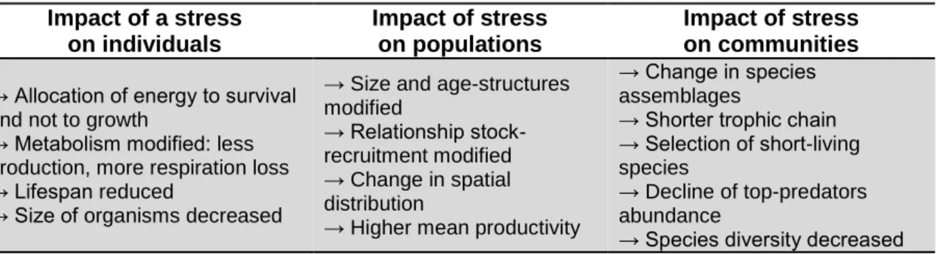
As the level of complexity of the ecosystem is increasing during maturation, the system would accumulate more energy through an increasing efficiency (Saint-Béat et al., 2015) and slower biomass flow transfers (Gascuel et al., 2008). Stress is suspected for altering the productivity and stability of marine ecosystems and may induce a return to a less mature system. Stress duration and intensity are expected to induce less stable and less productive ecosystems through faster biomass transfers and reduced transfer efficiencies. This will constitute the research hypothesis of our work and will be tested on Large Marine Ecosystems from 1950 to 2010. In fact, such stresses are in theory expected to modify the ecosystem at a global scale through several mechanisms. A stress modifies the metabolism at an individual scale and can enhance a higher respiration rate in order to maintain survival of the marine species (Table 1). Then, in the metabolic balance, the conversion rate of food into growth may decline. At the community level, stresses are causing natural selection of short-living species with fast but potentially less efficient energy transfers. The reduced abundance of top-predators is caused by lower energy availability in the top of the food web and may induce a reduced overall productivity (Odum, 1985).
Table 1 : Trends expected on individuals/populations/communities generated by stress (adapted from Odum, 1985)
Impact of a stress on individuals Impact of stress on populations Impact of stress on communities → Allocation of energy to survival
and not to growth
→ Metabolism modified: less production, more respiration loss → Lifespan reduced
→ Size of organisms decreased
→ Size and age-structures modified
→ Relationship stock-recruitment modified → Change in spatial distribution
→ Higher mean productivity
→ Change in species assemblages
→ Shorter trophic chain → Selection of short-living species
→ Decline of top-predators abundance
→ Species diversity decreased In this approach, we focus on the community level that expresses major changes in the ecosystem by succession of species through time series. Evidence for variations within the individual metabolism and growth and within populations have been highlighted in the scientific literature (Britten et al., 2016; Sumaila et al., 2011), but will not be considered here. The focus on the community level is useful to sick for trophic interactions and ecosystem functioning variability in terms of energy flows (Rombouts et al., 2013). The present research work focuses on how changes in species assemblages induced by fishing or climate change stresses modify the global functioning of marine ecosystems worldwide.
1.3 Theoretical parameters in ecology of the trophic ecosystem functioning
In order to examine the impact of intense stress, two parameters are being investigated. They both characterize the biomass flow within food webs from phytoplankton to top-predators. The first parameter, the trophic transfer efficiency (TE), is related to the ecosystem productivity. It represents the rate of biomass that is transferred in the food web
from one trophic level to the next. So, it results from the opposite of all the biomass loss that can occur during metabolism and the species life cycle (respiration, excretion, fishing, natural mortality other than predation). The second parameter is the speed of the biomass flow, also called kinetics, inversely proportional to the time necessary for a unit of biomass to cross the food web from one trophic level to the next.
The trophic transfer efficiency can be considered as an “indicator of the system status
and condition” (Libralato et al., 2004)
The concept of trophic transfer efficiency is largely used in ecosystem modelling, and discussed in the scientific literature. The trophic transfer efficiency is often fixed for the whole ecosystem: “Since (Lindeman, 1942), it has often been assumed that trophic transfer efficiencies in ecosystems vary around 10%” (Christensen et al., 1993). Several definitions of the transfer efficiency exist such as per trophic level “efficiency at which energy was passed from one trophic level to the next” (Lindeman, 1942), “proportion of prey production that is converted to predator production” (Jennings et al., 2002), or for the entire food web “transfer of energy from phytoplankton to progressively larger animals” (Barnes et al., 2010). Assumptions are made: “Transfer efficiency from mesozooplancton to fishes is also probably higher in less productive and clear oceanic waters than in more productive and turbid shelf and coastal waters” (Irigoien et al., 2014).
In theoretical ecology, the TE is expected to vary with the period of time (Libralato et al., 2004) and the type of ecosystem considered (Pauly and Christensen, 1995). Depending on which species or which part of the food web, the transfer efficiency might be variable: some species are more efficient than others (Straile, 1997). The food web efficiency could be a decreasing function of the trophic level (Christensen et al., 1993) or the species size (Jennings et al., 2002). However, even if we know a lot about this parameter in theory, in practice it is usually considered as a constant such as in ecosystem models (Tremblay-Boyer et al., 2011) or in ecosystem indicators calculation (Chassot et al., 2010; Christensen, 2000; Pauly and Christensen, 1995). The parameter variability is not enough explored. Here we will reconsider the models’ assumptions in order to see if the TE actually varies over the time-series and between geographical locations. The variability of the TE across trophic levels is also very few explored and calculated (Libralato et al., 2008) and will be investigated here. As the TE is increasing with the ecosystem development, the impact of stress would tend to abate the overall efficiency of the food web (Odum, 1985). The loss of complexity and return to a less mature system would disrupt the productivity.
“Flow kinetics is a key characteristic, partly determining the ecosystem’s response to human disturbances such as fishing pressure” (Gascuel et al., 2008)
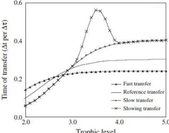
The kinetics traduces the speed of the trophic flow from one trophic level to the next, according to predation. This parameter, as a characteristic of the general biomass decreasing flow within the food web, is just as important and informative of the ecosystem functioning. “Quantifying flow kinetics appears as a key step in our understanding of ecosystems dynamics” (Gascuel et al., 2008). The speed of flows is the reverse of the time required to go up the food web (Figure 2). It is related to the life expectancy of organisms in its trophic class (Gascuel et al., 2011).
Following a steady-state hypothesis, the residence time may be accessed as the reverse of Production/Biomass ratio for a species, an ecosystem compartment or the entire food web (Gascuel et al., 2011; Schramski et al., 2015). This approach of the time, also developed in the EcoTroph model (Gascuel and Pauly, 2009) is considered here. The residence time of biomass particles is sensitive to ecosystems and temporal variability. For instance, the residence time in the food web is longer for coral reefs than for upwelling systems (Christensen et al., 1993). The residence time of carbon particles in a trophic compartment can raise with producer body mass (Schramski et al., 2015) and during the ecosystem development (Fath et al., 2004).
Fishing pressure would boost the speed in the ecosystem due to the reduction in life expectancy of exploited species and the selection of short-living species characterized by fast turn-over. This return to a less mature system would shorten the residence time of the biomass particles in the system. Climate change and elevating sea surface temperature are also expected to shorten this time of biomass transfer.
1.4 Research questions
Basically, the trophic transfer efficiency and the kinetics depend on the ecosystem structure and assemblages and from all species properties. Then, stress like climate change and fisheries are suspected to modify these parameters through – among other modifications – different species assemblages in the ecosystem. We developed here a way to assess the transfer efficiency and kinetics and to study their trends over time series. The purpose is to identify and possibly explain their variations depending on the fishing activities and climate change. As described by (Worm and Duffy, 2003), we are interested in two of the three aspects of the ecosystem: the quantity through the trophic transfer efficiency and the temporal stability, through the speed of biomass flows/residence time of biomass in the food web. Indeed, the quality of the ecosystem is not assessed here.
Studying the variability of theoretical functioning parameters allow to explore the following research questions:
Did changes in species assemblages, induced since 1950 by climate change and fishing pressure, modify the two major parameters of the food web functioning : the trophic transfer efficiency and the trophic kinetics ?
More specifically, this implies to answer the following sub-questions:
Are we able to identify such changes at the Large Marine Ecosystem scale using available data?
What are the main patterns of these changes?
Are they related to climate change and/or fishing pressure?
Do they express – as in Odum ecological theory – variations leading to less productive and less stable marine food webs?
Figure 2 : Time of transfer in the food web per
trophic level for various theoretical
kinetics/speeds of biomass flow (from Gascuel et al., 2005)
2. Method
2.1 Data, scale of the study
2.1.1 Sea Around Us catch database: worldwide marine ecosystems data
The database used for marine food webs species composition is the Sea Around Us (SAU) Project fisheries catch data (Pauly and Zeller, 2015). This catch data has been reconstructed starting in 1950 and until 2010 taking into account FAO declarations, small-scale fisheries, recreational fisheries, fisheries discards and illegal fishing or false declarations in order to get a better approach of the real impact of catch (Pauly and Zeller, 2015). Using catch data and not biomass or abundance information on species has two consequences. First, we consider only the exploited part of the ecosystem. For high trophic levels, most species are or can be fished and this exploited part of the biomass can be assumed very close (or similar) of the total biomass. In contrast, this is clearly not the case for low-trophic level species such as phytoplankton and zooplankton. Their influence cannot be studied here. This hypothesis has been tested on the North Sea ecosystem (Appendix II) thanks to the Ecopath model built by (Mackinson and Daskalov, 2007). It looks that biomass and catch give the same results, except for the low trophic-level species, as expected. Secondly, we do not consider changes induced by fishing strategies. We will discuss this assumption in the last part of this work, in light of our results.
In the objective of reducing the number of species for each ecosystem and to avoid bias linked to rare and poorly registered species, we selected only the species groups from the SAU data that represented at least 0.1% of the total catches at least one year between 1950 and 2010. For the North Sea, it divided the number of species by 2 (sensitivity analysis,
Appendix II). This method is often used at a global scale and is assumed to well represent
the ecosystem communities (Worm et al., 2009). This limit also allowed to get at least 95% of the catches every year for all the ecosystems.
All the trophic levels for taxonomic groups were also taken from the SAU Project. They were calculated from the most precise data available on FishBase (Froese and Pauly, 2016) and SeaLifeBase (Palomares and Pauly, 2016) for all the groups. The Sea Around Us dataset includes 2557 taxonomic groups. These groups can represent one species, one genus, one family, one order or one class.
2.1.2 Geographical scale: Large Marine Ecosystems
The spatial fisheries catch reconstruction from the SAU Project allows an ecosystem approach through the Large Marine Ecosystems (LMEs), ecosystem units defined by Sherman (1991). Nowadays, we count 66 LMEs (but 2 were taken out considering missing data for the Arctic and Antarctic Oceans). They correspond to coherent ecosystems defined by the bathymetry, the productivity, species assemblages and coastal areas limits (see the Large Marine Ecosystem official map in Appendix I). Coastal areas concentrate at least 80 to 90% of the total worldwide catch (Christensen et al., 2008): these ecosystems are representative of the major fisheries catch.
(USA), the Humboldt Current (South American upwelling ecosystem), the Gulf of Mexico, the Canary Current (Western Africa) and the Sea of Japan (Asia). Here, the purpose is to deeply analyze past changes in efficiency and speed of flows and their causes through various marine species assemblages since 1950.
Figure 3 : Worldwide map with the Large Marine Ecosystems boundaries from http://www.seaaroundus.org/
where are noticed the official LME number for the 6 chosen ecosystems (in blue) for the study (3: California Current, 5: Gulf of Mexico, 13: Humboldt Current, 22: North Sea, 27: Canary Current, 50: Sea of Japan) – the omitted LMEs in black.
A second statistical approach is leaded to test explicative factors for temporal variations in efficiency and speed, potentially affected by stress. The quantitative analysis is conducted on 56 of the 66 Large Marine Ecosystems, in order to include the ecosystems with the best data available (catch, climate data). Following Chassot et al., 2010, poorly documented LMEs were taken out: East China Sea, Yellow Sea, Chukchi Sea, Beaufort Sea, East Siberian Sea, Laptev Sea, Kara Sea, Antarctic, Hudson Bay and the Central Arctic Ocean (Figure 3).
2.1.3 Estimation of species parameters for all the Sea Around Us groups
Using SAU database and the LMEs, the following species parameters have been estimated: the von Bertalanffy growth coefficient, weight and length, varying with the geographical locations. Two large databases are used to get these ecological parameters: FishBase (Froese and Pauly, 2016) and EcoBase (Colléter et al., 2015). FishBase regroups ecological parameters for fish species. If the population traits are not available for the smallest geographical scale, we can focus on a larger one (Figure 4). If no parameter is available for the species, we will first look at other species geographically close from the same genus. If none parameters can be found, a larger taxonomic scale is used.
Figure 4 :Geographical and taxonomic scales included in the parameters estimation methodology
SeaLifeBase, a similar database for non-fish species has been considered (Palomares and Pauly, 2016). However, because it is not enough complete, an estimation of P/B, P/Q and Q/B ratios is taken from EcoBase, repository for a large number of Ecopath with Ecosim models where these ratios have been collected (Colléter et al., 2015). These estimations are not as precise as for the fish species: no geographical precision and for large groups of species only (Table 2).
Table 2 : Estimation of parameters of interest per group of species from the Ecobase depository
The growth parameters used such as the growth rate, the asymptotic length and weight are considered as constants over the whole time-period. The individual variability is not included. This methodology allowed us to get all the parameters for all the taxonomic groups selected from the SAU catch database for each LME. Because the taxonomic groups are not as precise all the time or because the parameters do not exist or are not reported into the database, a level of uncertainty and imprecision is existing. However, the methodology permitted to get the highest precision possible considering the taxonomic scale and level of the study.
2.2 Trophic-level based approaches: spectrum and indices
The trophic-level based approach was identified as adapted to answer the research question considering that species are not directly considered here but their trophic level by class. The variability of each trophic class by variations is the species assemblages, initiated by the TL classification of species (Gascuel et al., 2011) reflects the global variability. Then, from the species trophic level, we will transform the data into trophic class. Through this trophodynamic approach, partial transfer efficiency and speed of biomass flows are estimated.
2.2.1 Calculating ecological biomass flow parameters
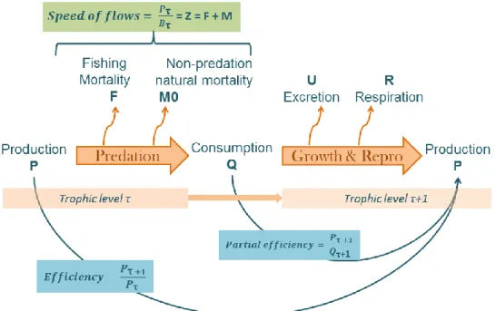
The speed of flow of each species is identified as the ratio P/B, production by biomass (TL.year-1) (Gascuel et al., 2008). Under equilibrium assumption, it is the total of mortalities noted Z, as the sum of the natural mortality and the fishing mortality (Allen, 1971) (Figure 5).
Here, we only consider the natural mortality M. Thus, we analyze the changes in flow kinetics induced by changes in species assemblages occurring at each trophic level, independently of the level of fishing pressure. In other word, the changes in species assemblages will be translated into changes in natural mortalities M per trophic class, as a different mortality rate can be associated to each species. M delivers the residence time of a species in the ecosystem. For short time living species, the natural mortality and the speed of flow are high. Numerous natural mortality empirical equations exist in order to calculate M directly from growth parameters. We tested some of them and led a sensitivity analysis to see if they actually influence the final results for the North Sea LME (Appendix II).
Groups of species
Abalones, Clams, Mussels, Oysters, Sessile molluscs, Sea urchins, Starfish, Echinoderms, Cnidarians, Sea Cucumbers, Sea Snails, Shrimps, Lobsters, Crabs, Crustaceans, Squids,
Octopuses, Cephalopods, Cuttlefishes, Cirripedes, Miscellaneous aquatic invertebrates, Miscellaneous crustaceans
Figure 5 : Predation process with all the kind of loss occurring in the energy transmission between the prey and
its predator (adapted from Gascuel et al., 2008)
The following equation initially fitted on FishBase data (Gascuel et al., 2008) has been selected as a reference one.
𝑃
𝐵
= 1.06 × 𝑒
0,018 ×𝑇
× 𝐾
0.75(1)
Where P/B is the speed of flows (TL.year-1), T in the temperature (°C) and K von Bertalanffy growth coefficient (year-1)
The trophic transfer efficiency, as the ratio of two production rates between preys and predators (Figure 5), will not completely be assessed here. The ratio P/Q, Production by Consumption, is directly calculated from P/B ratio as following:
(
𝑃 𝑄)
𝜏=
(𝑃 𝐵⁄ )𝜏 (𝑄 𝐵⁄ )𝜏=
𝑠𝑝𝑒𝑒𝑑 𝑜𝑓 𝑡ℎ𝑒 𝑏𝑖𝑜𝑚𝑎𝑠𝑠 𝑓𝑙𝑜𝑤 𝑓𝑜𝑜𝑑 𝑐𝑜𝑛𝑠𝑢𝑚𝑝𝑡𝑖𝑜𝑛 𝑟𝑎𝑡𝑒(2)
For getting P/Q, the food consumption ratio Q/B was estimated using the following empirical equation(Palomares and Pauly, 1998):
log (𝑄 𝐵) = 7,964 − 0,204 × log(𝑊𝑖𝑛𝑓) − 1,965 × 1000 𝑇 ′ + 0,083 × 𝐴𝑅 +0,532 × ℎ + 0,398 × 𝑑
(3)
Where Q/B is the food ingested relative to its biomass, Winf is the asymptotic weight from the Von Bertalanffy models (g), T is the water temperature (°K), AR is the aspect ratio of the caudal fin, h=1 if the species is herbivorous, d=1 if the species eats detritus
P/Q, being a partial trophic efficiency, is considered as the “gross food conversion efficiency” (Christensen et al., 1993). This ratio focusses on the effects that species composition might have on total losses related to respiration. So, it is strongly linked to the total transfer efficiency. Nevertheless, it should be noted that this partial efficiency does not consider the variability emerging from non-predation mortalities (Figure 4). In other words, the selection of
species with large predation mortalities (i.e. trophic dead-end species) caused by human-induced stresses will not be identified in our analysis.
It has been previously demonstrated that the respiration rates changes with time, especially with fishing activities and climate change (Cheung et al., 2012). The TE “depends on non-predation mortality, excretion and respiration” (Gascuel and Pauly, 2009) and it seems that respiration is the parameter that influences the most the efficiency (Christensen et al., 1993). Then, by looking into the various combinations of species assemblages per TL and trophic class, the partial efficiency variability will emerge from each species metabolic properties.
2.2.3 From species to the trophic class as units of study
P/B and P/Q parameters were estimated per trophic class using a trophic spectra approach following Gascuel et al., 2005. For that purpose, the R package EcoTroph was used (Colléter et al., 2013):
Figure 6 : Catch spectra for the North Sea – Left: Spectrum of the catches in 1990 per species (each color is a species) – Right: Spectrum of the catches from 1950 to 2010 every five years
A spectrum is the result of a transformation from the species data to trophic class data. From species catches and TL, a smooth function splits the value of interest through a log-normal distribution on the trophic levels. Thus, the value of interest is not distributed by species but by TL based on trophic class with a Δ𝜏=0.1 range. This trophic representation method of the ecosystem is useful to understand where the fisheries catch happen in the food web (Gascuel et al., 2005). For example, in the North Sea, catch are the most important in the trophic class 3.0-3.5 and changed over time (Figure 6). In order to study the time of residence of species in the ecosystem and the partial efficiency, we look at P/B and P/Q ratios spectra. For each trophic class [𝜏 ; 𝜏 + ∆𝜏 [ mean P/B and P/Q ratios are calculated proportionally to the related catch amount of each species i:
(
𝑃 𝐵)
𝜏=
∑ (𝑖 𝑃𝐵)𝑖 ×𝑌𝑖,𝜏 ∑ 𝑌𝑖 𝑖,𝜏and
(
𝑃 𝑄)
𝜏=
∑ (𝑖 𝑄𝑃)𝑖 ×𝑌𝑖,𝜏 ∑𝑖𝑌
𝑖,𝜏(4)
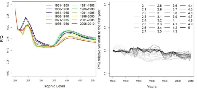
Where Y are the catches, P/B the speed of flows and P/Q the partial efficiency of species.Figure 7 : Spectra for the North Sea – Left: P/Q spectrum per trophic level every 5 years – Right: relative P/Q
values spectrum per year for each trophic class (step = 0.1), each value per year is divided by the P/Q (1950) Then, for each ecosystem, we calculate the spectra of both parameters for which we can already observe temporal variations per trophic class (Figure 7). This data transformation is a key step in our trophodynamic approach to analyze the changes of parameters along the time-series at a global scale or by having a focus on certain parts of the ecosystem. Then, another transformation of the data into global ecosystem indices has been realized to lead the LME meta-analysis.
2.2.4 From parameters per trophic class to integrated ecosystem indices
P/Q is a ratio without unit. We create a cumulated index that allowed quantifying the proportion of production transferred to the top of the food web. Then, if this index is decreasing with time, it shows that high-TL species are having less food available and that the ecosystem lost in productivity.
The Efficiency Cumulated Index (ECI) refers to the cumulated efficiency: from the multiplication in the index, the partial efficiency, just as in the food web, is progressively integrated from low trophic level parts of the food web to the top.
𝐸𝑓𝑓𝑖𝑐𝑖𝑒𝑛𝑐𝑦 𝐶𝑢𝑚𝑢𝑙𝑎𝑡𝑒𝑑 𝐼𝑛𝑑𝑒𝑥(𝑦) =
∏
(
𝑃 𝑄)
𝜏,𝑦∆𝜏 𝜏=𝑏 𝜏=2.0∏
𝜏=𝑏𝜏=2.0(
𝑄𝑃)
𝜏,1950∆𝜏(5) Δ𝜏 is the trophic-level step used from one trophic level class to the upper one (here Δ𝜏=0.1). The coefficient b corresponds to the upper trophic level chosen (2.5/3.0/3.5/4.0/4.5).
The Time Cumulated Index (TCI), reversly proportionate to the speed of flows, refers to the time necessary to go up the food chain:
Regarding the speed of flows P/B, we developed another way to look at it based on the EcoTroph approach (Gascuel and Pauly, 2009). The inverse of this ratio captures the time necessary for the biomass to go along the food chain. Thus, we sum up all the times from all trophic levels and it indicates how long it takes to go to the top of the food chain from TL=2.0
𝑇𝑖𝑚𝑒 𝐶𝑢𝑚𝑢𝑙𝑎𝑡𝑒𝑑 𝐼𝑛𝑑𝑒𝑥 (𝑦) =
∑ 𝛥𝜏 (𝑃𝐵)𝜏,𝑦 𝜏=𝑏 𝜏=2.0 ∑ 𝛥𝜏 (𝑃𝐵)𝜏,1950 𝜏=𝑏 𝜏=2.0(6)
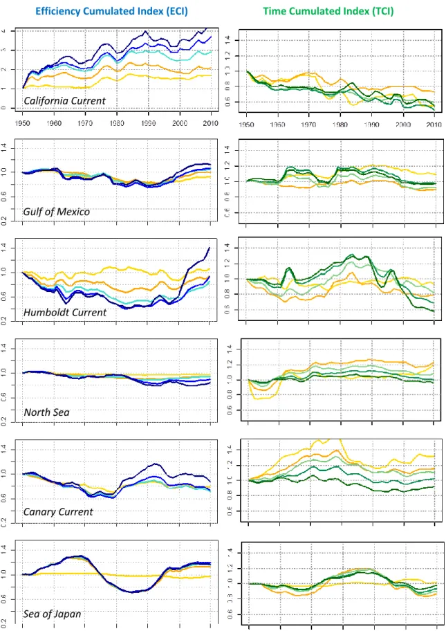
This TCI can be interpreted as a factor of stability in the ecosystem, but this will be more discussed later. These indices are calculated relatively to the first year of the time series so we can see their relative variations over time, standardized the same way for all LMEs. We calculate here the index from TL=2.0 to TL=4.0 as a reference. Indeed, b=4.0 is an interesting limit because it shows how much of the biomass is available for top-predators in the ecosystem. We also tested different limits to search for the progressive index changes along the food chain.
2.3 Choice of explanatory parameters for fishing pressure and climate change 2.3.1 Fishing pressure measures
Because no access to reliable fishing effort data at this global LME scale is available yet from the SAU Project, several fishing pressures indices are investigated:
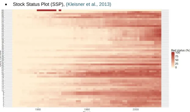
Stock Status Plot (SSP), (Kleisner et al., 2013)
Figure 8 : Top – Time-series of the % of over-exploited and collapsed assessed stocks per Large Marine Ecosystem from 1950 to 2010
This index of fishing pressure is available for each LME on the SAU website, where the method of assessment is detailed (www.seaaroundus.org/). It measures the proportion in number of collapsed or overexploited stocks in each LME (Figure 8). This measure relies on two strong disputable hypotheses: the highest pick of catches in the time-series is considered as the maximum sustainable catches amount, while it can come from changes of fisheries strategy or fisheries management. Decreases in catch are assumed to be the result of over-exploitation of the related population.
The Primary Production Required for fisheries (PPR) (Pauly and Christensen, 1995) is the amount of carbon needed to produce the catches:
𝑃𝑃𝑅
𝑘= ∑
(
𝑌𝑖𝑘 9) ×
𝑛 𝑖=1(
𝑇𝐸𝑘1)
𝜏𝑖−1 (7)Where PPRk is in t C.km-2.year-1 and k is the LME, i the species, Yik the catch of species i in LME k, TE is the Transfer Efficiency, here assumed to be equal to 10% and 𝜏 the trophic level of the species. The PPR value is not directly used, but the ratio PPR/PP (%) (where PP is the Primary Production) as the fishing pressure index. As a reference, a constant PP value is attributed to each LME from the Eppley correction observation data. However, the PPR/PP values (%) are extremely high for some ecosystems. This index should vary between 0 and 30-50% (Pauly and Christensen, 1995; Swartz et al., 2010), and our results show much higher variations (Appendix III). More particularly, PPR/PP is sensitive to the trophic transfer efficiency value used (Watson et al., 2014) and the primary production data (Cury et al., 2005). This led to a sensitivity analysis (Appendix III).
Lindex (Libralato et al., 2005)
𝐿
𝑖𝑛𝑑𝑒𝑥,𝑗,𝑘= −
𝑃𝑃𝑅𝑘 × 𝑇𝐸𝜏𝑐 (𝑘)−1 𝑃𝑃𝑘×ln (𝑇𝐸) (8)Where k is the LME, PPR is the primary production required for fisheries, TE is the transfer efficiency, 𝜏𝑐 is the mean trophic level of catches per LME and PP is the primary production from Eppley.
Again the transfer efficiency value is considered as 10% per ecosystem as a reference value. Lindex is constructed on a different way than the PPR, informing differently on the impact of fishing: it quantifies the loss in the secondary production in the ecosystem, due to fishing at the various trophic levels.
The Mean Trophic Level (MTL), (Pauly, 1998) of catch informs on the mean food web level of the fisheries catch
𝑀𝑇𝐿
𝑗,𝑘=
∑𝑛𝑖=1𝑌𝑖,𝑗,𝑘× 𝜏𝑖 ∑𝑛𝑖=1𝑌𝑖,𝑗,𝑘(9)
Where MTLj,k is the mean trophic level per year j and per LME k, Yi,j,k the catches per species, year
and LME, 𝜏𝑖 is the trophic level per species i.
Fishing in Balance (FIB) index, (Pauly, 2000) informs on the deployment of the fisheries on an ecosystem through an integrative construction relative to 1950:
𝐹𝐼𝐵
𝑗,𝑘= 𝑙𝑜𝑔10 (
∑𝑛𝑖=1𝑌𝑖,𝑗,𝑘 × 10𝜏𝑖∑𝑛𝑖=1𝑌𝑖,1950,𝑘× 10𝜏𝑖
)
(10)
Where FIBj,k is the index per year j and per LME k, Yi,j,k the catches per species, year and LME, 𝜏𝑖 is
the trophic level per species i.
2.3.2 Climate change data
Several sources of climate data have been considered, from satellite observations to models. As observations, the Eppley data (sbir.nasa.gov) have been used (as aggregated per Large Marine Ecosystems) for mean values over the observed time-series in order to get the best climate information. For the variation of the values from 1950 to 2010, GFDL model data was used (Geophysical Fluid Dynamics Laboratory, NOAA, www.gfdl.noaa.gov).
2.3.3 Other explanatory variables
Along the study, it appeared interesting to include as well other explanatory variables that inform differently on the ecosystem functioning: the proportion of fish, cephalopods and shrimps species in the catches, calculated all from the SAU database (Appendix III).
2.4 Statistical analysis of the index variations 2.4.1 Dynamic Factor Analysis
The Dynamic Factor Analysis (DFA) has been conducted in the following purpose: showing the relationship of the ecosystems time-series to temporal covariates trends. It is a multivariate time-series analysis, and it helps to put in light the major trends in the ecosystems. The DFA allows studying the correlation to the worldwide temporal trend in fishing pressure and climate change.
Using the MARSS R package (Holmes et al., 2013), several models were tested on the ECI only. Already used for LMEs meta-analysis with SAU data (Mcowen et al., 2015) and for other fisheries and marine species temporal trends (Mills et al., 2013; Zuur et al., 2003; Zuur and Pierce, 2004), this method was selected here in order to identify the major trends in the ECI common to all LMEs, and to include explanatory variables as additional trends. From the 1950-2010 time-series, we analyzed the temporal variations on the 56 LMEs. The DFA tests
m common trends within the time-series and can contain covariate effects. Basically, the
observations (ECIt) are considered as a linear combination of m trends (x), explanatory covariates (d) and noise (v). The model is constructed in the following way:
𝐸𝐶𝐼
𝑡= 𝑍𝑥
𝑡+ 𝑎 + 𝐷𝑑
𝑡+ 𝑣
𝑡(11)
Where ECIt are the observations at year t, Z the factor loadings, xt, the matrix of m trends, a the offsets, D the matrix containing the covariates effects on the observations, dt the covariates matrix at year t, vt the observations errors at year t as the noise component. This noise follows a multivariate normal distribution, centered on 0, with various possible variances and covariance relationships. The matrix of variance needs to be tested with several options during the model run (Zuur et al., 2003). We tested several models, and selected the best one/ones by their corrected Akaike’s information criteria (AICc), distinguishing the model getting the best number of trends and the best covariates to fit the ecosystem time-series. In order to restrict the test of models, we set the common trends from 2 to 5. The data was standardized by the mean on the time-series and the standard deviation (Appendix VII, Fig.1). Regarding the noise component, we choose to test a “diagonal and unequal” variance matrix: the ecosystems have unequal variance and no covariance (considering that LMEs have the same variance is not realistic). The covariates added to the model are mean of all ecosystem trends per year. Because we do not add the proper ecosystem covariate but the global worldwide signal, the model answers to the question: are the LMEs correlated / influenced by the worldwide temporal signal in fishing pressure and climate change? Five covariates have been tested separately into the Dynamic Factor Analysis (DFA) model. Then, two covariates were selected for a model incorporating climate change effects and fishing pressure effects.