Simulation of a passive house coupled with a reversible heat pump/organic Rankine cycle unit

(1)

9th International Conference on System Simulation in Buildings, Liege, December 10-12, 2014

Simulation of a passive house coupled with a heat pump/organic

Rankine cycle reversible unit

1. ABSTRACT

This paper presents a dynamic model of a passive house located in Denmark with a solar absorber, a horizontal ground heat exchanger coupled with a HP/ORC unit. The HP/ORC reversible unit is a module able to work as an Organic Rankine Cycle (ORC) or as a heat pump (HP). There are 3 possible modes that need to be chosen optimally depending on the weather conditions, the heat demand and the temperature level of the storage. The ORC mode is activated, as long as the heat demand of the house is covered by the storage, to produce electricity based upon the heat generated by the solar roof. The direct (free) heating is used when the storage cannot cover the heat demand of the house. Finally, when direct heating is not sufficient to cover the heat demand because of poor weather conditions, the HP mode is activated.

Dynamic simulations of the whole system are presented for different typical days of the year in Modelica language. A peak of 3.28 kW of power is reached in ORC mode with a heat input of 59.5 kW from the solar roof (23.9 kWh are produced during a typical summer day). In a representative winter day, 5.81 kWh are consumed by the heat pump with a daily average COP of 4.3. Conclusions regarding control strategies and enhancement of the global system are drawn. A control strategy with a low storage temperature set-point (50˚C) allows reducing electrical consumption from 20% up to 60% when compared to higher set-point (60˚C). The system performance to produce power could also be optimized if an extra tank is included to store heat uniquely to produce electricity with the ORC during the peak electricity consumption. Finally, the paper points that this technology is a promising way to achieve Plus Energy Building at low price and higher efficiency compared to competitive systems, as photovoltaic-thermal solar heat pump.

Keywords: Net Zero Energy Building, Reversible Heat Pump/Organic Rankine Cycle, Solar

energy.

2. INTRODUCTION

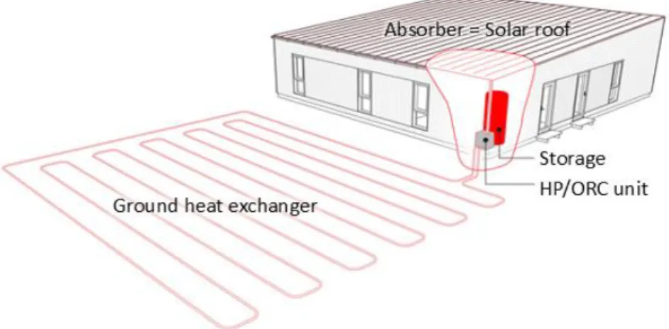
According to the European commission directive (European commission, 2011), all new buildings in Europe should be Net Zero Energy Building from 2019 (Jagemar et al, 2010; Kurnitski et al, 2014). In this context, heat pumps should play a major role (Bettgenhäuser et al, 2013; Hepbasli and Yalinci, 2009). This paper investigates a heat pump which presents the ability to operate as an organic Rankine cycle without increasing the costs significantly (Dumont, 2014(a)). This reversible HP/ORC unit is coupled to a passive house (Figure 1) with a large solar absorber and a horizontal ground source heat exchanger (Innogie, 2013).

(2)

Figure 1: The reversible HP/ORC unit integrated in the house (Dumont, 2014)

The paper is organized into 4 parts. Firstly, the reversible HP/ORC unit is introduced. Then, the models of the components are presented. Thereafter, results from simulation on typical days are described and discussed. Finally, prospects and conclusions are discussed.

A simplified scheme of the system, operating in ORC mode, is presented in Figure 2.

Figure 2: Simplified scheme of the unit (ORC mode) (Dumont, 2014(a))

Dynamic modelling of the whole system including the solar roof, the ground source heat exchanger, the storage tank, the reversible HP/ORC unit and the house is necessary to simulate the performance of the system. These simulations help to evaluate the performance with different climates, house envelope, storage size and control strategies.

3. MODELING

3.1 Introduction

In this chapter, the model of each sub-system is described. The control strategy is also introduced.

(3)

In the law of conservation of energy, if the mass and volume (or time constant) are negligible, then the equation becomes independent of time. Thus, it is important to evaluate the inertia of each component, fast transients should not be taken into account because their influence is negligible. Furthermore, the system composed of sub-systems having very different time constant requires very long simulation time. Time constant (τ) are evaluated experimentally or estimated with Eq. 1 and compared in Table 1.

In this equation, M is the mass of the system, 𝑚̇ is the typical flow and 𝛥𝑇 is taken equal to 10°C. This results from an energy balance assuming that flow and specific heat are constant. The time constant is reached when the increase in temperature has reached 63% of its final value.

Table 1: Time constant of the different sub-systems

Sub-system Method Time constant [min]

Reversible HP/ORC unit Experimentation 5

Solar roof Eq. 1 18

Storage Eq. 1 87

House Simulation 3133 (50h)

Ground source heat exchanger Experimentation (see section 3.6)

The inertia of the unit is, therefore, neglected because of its very low time constant. Solar roof, house and storage dynamics are of course modeled. The ground source heat exchanger inertia is discussed in section 3.6.

3.2 Reversible HP/ORC unit

The unit has been tested in a wide range of conditions experimentally (Dumont, 2014(a)). Following that, semi-empirical models have been calibrated to fit the measurements. In heat pump mode, the sub-cooling is imposed at 2 K and the over-heating at 6 K. In ORC mode, the sub-cooling is imposed by the NPSH (net positive suction head) of the pump and the over-heating is optimized (by adjusting the pump speed) to maximize the electrical power production. As shown in Dumont (2014(b)) the polynomials used to evaluate the outputs of the reversible unit.

3.3 Storage

The water tank storage system is described by partial differential equations which consist of derivatives with respect to time and space for an incompressible fluid. The spatial equations are discretized according to the finite volume method. Dymola/Modelica solves the dynamic part of those equations using DASSL solver.

𝜏 = 0.63. 𝑀. 𝛥𝑇 𝑚̇

(4)

Figure 3 shows the structure of the tank model. The water tank model can be divided into three subsystems: tank subsystem, one parallel internal heat exchanger subsystem and one counter flow internal exchanger subsystem.

Figure 3: Water storage unit with internal coils diagram.

The tank subsystem comprises the water tank, a top outlet and the bottom inlet that are part of the floor heating circuit. The tank is discretized using a modified version of the incompressible Cell1Dim model adding an additional heat port, which represent a model of a stratified tank and ambient losses (Quoilin et al, 2014). This subsystem is discretized into 20 cells, where the energy and mass conservation equations are applied. The momentum balance is neglected and the pressure is assumed to be constant in the whole tank. Each layer is described by one temperature variable. Each control volume takes into account water inflows, water outflows and conductive heat transfers with neighboring layers and with the environment.

The heat exchangers are modelled using the Flow1Dim component (Quoilin et al, 2014) and a wall component. The bottom heat exchanger - part of the reversible unit circuit and responsible for supply heat in DH and HP modes - is modelled using an original Flow1Dim component and a wall component. The top heat exchanger - the domestic hot water coil - is discretized using a modified version of Flow1Dim with a Countcurr component (Quoilin et al, 2014).

The fluid properties for the selected medium, StandardWater, are computed using the ThermoCycle library (Thermocycle, 2014). The dimensions and thermal constant of the tank model are summarized in Table 2.

Table 2: Water tank with two heat exchangers model parameters

Parameter Value Parameter Value

Tank total height [m] 1.44 Top Heat exchanger area (one side) [m2_] _2.5

Height bottom HX inlet [m] 0.54 Tank capacity [m3_] _0.5

Height bottom HX outlet [m] 0.09 Internal volume bottom HX [m3_] _0.011

Height top HX inlet [m] 0.09 Internal volume top HX [m3_] _0.025

Height top HX outlet [m] 1.225 U-value between inside of tank and ambient[W/m2_K]

(5)

Total heat exchange area of tank with ambient [m2_] _3.27 _{U-value of the heat exchanger[W/m}2_K] ₄₀₀₀

Bottom Heat exchanger area [m2_] _1.8

3.4 Solar roof

Since the recently patented roof (Innogie ApS, 2013) is being tested for the first time, no performance data is available and the solar roof is modeled with the classical correlation (Eq. 2) based on the ambient temperature (𝑇_𝑎𝑚𝑏) and on the mean temperature of the heat transfer fluid (𝑇_𝑚) with the area (A = 138.8 m2) of the roof and the solar irradiance absorbed by a collector per unit area of absorber (I). U is evaluated through the model of Klein (Klein, 1975). Finally the energy balance (Eq. 3) allows to evaluate the exhaust roof temperature with the mass M (104.6 kg), the specific heat (𝐶𝑝), and the mass flow rate of the working fluid, in

this case 30% glycol based water solution (𝑚̇).

𝑄̇_𝑐𝑜𝑙 = 𝐴(𝐼 − 𝑈(𝑇_𝑚− 𝑇_𝑎𝑚𝑏)) 2

𝑀. 𝐶_𝑝 . 𝑑𝑇_𝑚 = 𝑄̇_𝑐𝑜𝑙− 𝑚̇. 𝐶_𝑝 . (𝑇_{𝑤,𝑟𝑜𝑜𝑓,𝑒𝑥}− 𝑇_{𝑤,𝑟𝑜𝑜𝑓,𝑠𝑢}) 3

3.5 House model

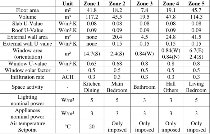
The present simulation model relies on a simplified multi-zone building model. The building is divided into 5 zones based on the house layout and the use of the spaces. The main characteristics of the building are presented by zone in Table 3.

Table 3: House main characteristics

Unit Zone 1 Zone 2 Zone 3 Zone 4 Zone 5

Floor area m² 41.8 18.2 7.8 19.1 45.7

Volume m³ 117.2 45.5 19.5 47.8 114.3

Slab U-Value W/m².K 0.08 0.08 0.08 0.08 0.08

Roof U-Value W/m².K 0.09 0.09 0.09 0.09 0.09

External wall area m² none 20.4 4.5 24.8 41.5

External wall U-value W/m².K none 0.15 0.15 0.15 0.15

Window area (orientation) m² 14.7(S) 2.4(S) 0.84(W) 0.84(W) 0.84(N) 6.7(E) 2.4(S) Window U-value W/m².K 0.63 0.68 0.8 0.8 0.8

Window solar factor - 0.5 0.5 0.5 0.5 0.5

Infiltration rate ACH 0.3 0.3 0.3 0.3 0.3

Space activity - Kitchen

Dining Main Bedroom Bathroom Hall Others Living Bedroom Lighting nominal power W/m² 5 5 3 3 5 Appliances nominal power W/m² 3 3 3 3 3 Air temperature Setpoint °C 20 Only imposed Only imposed Only imposed Only imposed

(6)

in zone 1 in zone 1 in zone 1

in zone 1

The Modelica model diagram of the house is presented in Figure 4. It is composed of models developed based on the Modelica Standard Library model (version 3.2) and also use the “MixingVolume” and “RadiantSlabs.SingleCircuitSlab” models developed in the Modelica library “Buildings” (Wetter et al, 2013). Hourly schedules are associated to the occupancy, the domestic hot water use, the lighting and appliances in each zone (Bertagnolio, et. al., 2013). The weather data used for the external temperature and the solar irradiance are provided by the DMI - Danmarks Meteorologiske Institut - (Wang et al, 2010).

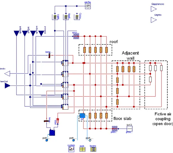
Figure 4: House model diagram in Dymola/Modelica

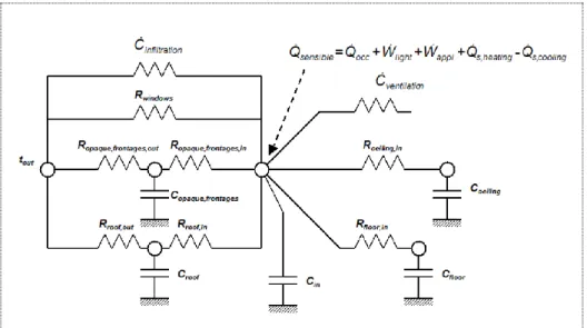
Each zone model is based on an equivalent R-C network including 5 thermal masses (Masy, 2006), corresponding to one occupancy zone, surrounded by external glazed and opaque walls (Figure 5).

(7)

9th International Conference on System Simulation in Buildings, Liege, December 10-12, 2014 Figure 5: Zone Model – Equivalent R-C Network Model

Massive walls are simulated using first order R-C “two-port networks”. A 2RC module is associated to each massive wall (Figure 6). The parameter of each “two-port network” are adjusted in order to produce wall admittance transmittance for a 24 hour period (Masy, 2006). The wall stationary U-value equals the invert of the whole two-port resistance. Ventilation system were not considered by means of computational simulation at this stage. To control indoor temperature rise a louver system is included.

Figure 6 - Capacitive wall and equivalent Dymola/Modelica model diagram

A PID controller controls the floor heating flow to regulate the ambient temperature (zone 1) inside the house close to the set point which is chosen equal to 20°C.

3.6 Ground heat exchanger

The ground heat exchanger is composed of a 300 meters long circuit disposed one meter deep in the ground. 36 thermocouples are disposed over the whole system (on third is 0.5 meter depth, the second third at 1 meter depth and the last one at 1.5 meter depth). Measurements in a second basis on the horizontal ground source heat exchanger showed that the ground temperature is very stable whatever the heat input/output. This temperature varies from 7°C in winter to 12°C in summer (day 182) with fall and spring temperatures of 10°C. For the moment, the temperature of the ground exchanger is therefore imposed following the measurements.

(8)

3.7 Global model

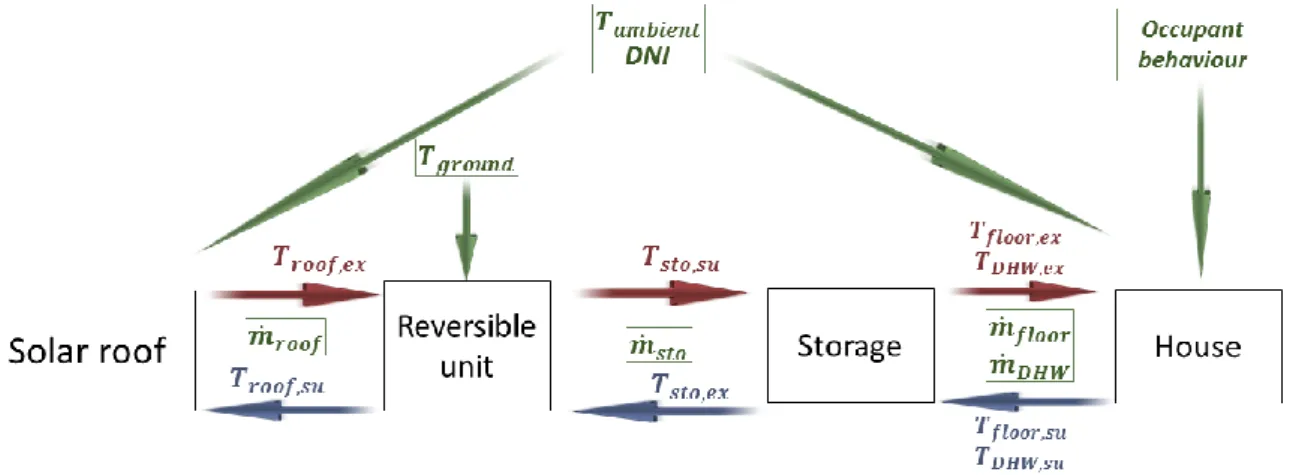
Figure 7 presents the flowchart of the global model combining the storage, building, roof, reversible unit and ground. The external inputs are meteorological data (ambient temperature and Direct Normal Radiation on hourly basis– Wang et al, 2010) and occupant behavior in the house (detailed in house model sub-section). The time step is fixed at 900 s. The consumption of auxiliary pumps is neglected, they represent less than 10% of the system consumption. Some parameters have to be fixed: Roof water flow, ground water flow, storage water flow and temperature set points of the storage. Practically, the following values are used for the flow based on real values measured in the house:

- Roof water flow = 0.6 kg/s, - Ground water flow = 1.5 kg/s, - Storage water flow = 0.6 kg/s - Floor water flow = 0.4 kg/s.

These flows should be optimized in future investigations to increase the energy efficiency of the system (Wystrcil, 2013). The influence of the set points values of the storage is investigated later (section 4.4).

Figure 7: Flowchart of the global model

3.8 Control strategy

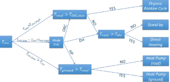
The control strategy is based on the following idea: Ensure the heat demand is covered while maximizing the net electricity production (Figure 8). That is the reason why the first control variable which is used is the storage temperature.

If the storage control temperature (𝑇_𝑠𝑡𝑜) is below a fixed low temperature threshold (𝑇𝑠𝑡𝑜,𝑙𝑜𝑤), the heat pump mode is activated to guarantee the space heating (SH) and

the domestic hot water (DHW). The heat pump cold source is the ground heat exchanger or the solar roof depending on which one is the warmest. If the storage control temperature is above the high temperature threshold (𝑇𝑠𝑡𝑜,ℎ𝑖𝑔ℎ), the ORC mode is activated if the roof

temperature is above the minimum temperature to get a net electrical production (𝑇𝑂𝑅𝐶,𝑚𝑖𝑛).

If the storage control temperature lies between the high and low threshold, the former mode is kept to avoid excessive chattering between modes reducing performance and reliability in practice. Finally, the by-pass mode is used if the storage temperature cannot be increased and

(9)

if the ORC mode is not able to produce a positive net electricity production. In the by-pass mode, only the roof pump is running to homogenize the roof temperature. This control strategy is relatively simple and should be improved in future works.

Figure 8: Control strategy of the global model

4. RESULTS FROM SIMULATIONS

Three typical days are simulated to evaluate the behaviour of the system with different inputs: a winter day (day 1), a spring day (day 62) and a summer day (day 182). To ensure steady-state conditions and for initialization each simulation is started 3h before the day considered. The two set points of the storage (𝑇_{𝑠𝑡𝑜,𝑙𝑜𝑤} and 𝑇_{𝑠𝑡𝑜,ℎ𝑖𝑔ℎ}) are 40°C and 50°C in this section. For each simulation, the following variables are plotted:

- Storage temperature from 10th cell (𝑇_{𝑠𝑡𝑜,𝑐𝑡𝑟𝑙}), - Outdoor temperature (𝑇_𝑜𝑢𝑡),

- House ambient temperature – zone 1 (𝑇_{ℎ𝑜𝑢𝑠𝑒}), - Exhaust roof temperature (𝑇𝑟𝑜𝑜𝑓,𝑒𝑥),

- Heat flow for floor heating (𝑄̇_{𝑓𝑙𝑜𝑜𝑟}), - Heat flow for domestic hot water (𝑄̇𝐷𝐻𝑊),

- Heat flow from unit (𝑄̇_{𝑢𝑛𝑖𝑡}),

- Electrical unit power consumption(-)/production(+) (𝑊̇_𝑒𝑙),

The mode in operation is detected by looking at the power and heating variables. If electrical unit power consumption is negative (resp. positive), it means that HP (resp. ORC) mode is activated. If heat flow coming from unit is positive and there is no electrical consumption, then DH mode is operating. Finally, in all the other cases, the bypass mode is enabled.

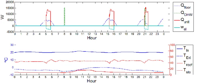
4.1 Winter - Day 1

Figure 9 shows the regulation mechanism during the first day of the year. When the storage temperature decreases down to the low threshold value (40°C) because of SH and/or DHW demand, the heat pump is activated to heat the storage to the high temperature threshold

(10)

(50°C). This control leads to 3 starts of the HP using the ground heat exchanger as heat source. The total electrical consumption of the heat pump is 5.81 kWh, leading to a daily average COP of 4.34 (Eq. 4).

𝐶𝑂𝑃𝑢𝑛𝑖𝑡 =

∫(𝑄̇ℎ𝑝+ 𝑄̇𝑑ℎ) 𝑑𝑡

∫ 𝑊̇𝑒𝑙 𝑑𝑡

4

The ambient temperature in the house is fairly well regulated around the set point (20°C) thanks to the regulation of the floor heating flow.

Figure 9: Dynamic simulation of the reversible unit coupled to a passive house for the 1st day of the year

4.2 Spring - Day 62

Figure 10 shows the main inputs and outputs for a typical spring day. In the morning, the HP is needed to keep the storage temperature higher than the low threshold temperature (40°C). From 10 AM to 12 PM, the direct heating increase the storage temperature until the storage temperature reaches the roof temperature (60°C). This heat coming from the roof allows to avoid the starting of the HP before next day. The electrical consumption of the HP is 1.68 kWh, leading to a daily 𝐶𝑂𝑃𝑢𝑛𝑖𝑡 of 10.48 (Eq. 3).

(11)

Figure 10: Dynamic simulation of the reversible unit coupled to a passive house for the 62nd

day of the year

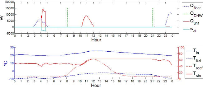
4.3 Summer – Day 182

Figure 11 shows the main variables for a typical summer day (182nd_{day). Different inferences}

can be drawn. Firstly, the only heat demand affecting the storage is the DHW (at 8h and 21h) because the house temperature is always above the temperature set point (20°C). It leads to the use of only two modes (ORC and bypass). Direct heating is used only a few decades of minutes to heat the storage when the temperature is below the low threshold value (not necessary all the days, see Figure 11). The ORC mode is activated as soon as the roof temperature reaches 70°C (i.e. the minimum value to start the ORC). The electrical production of the ORC reaches a maximum of 3.28 kW with a heat input on the roof of 59 kW (23.9 kWh are produced by the ORC during day 182). This leads to an efficiency of 5.5% to be compared with the theoretical one (7.5%). The main reason is that the model used for the ORC is based on the performance of the unit tested experimentally. Several factors like low expander efficiency, high sub-cooling and no thermal insulation explain this difference (see Dumont et al 2014(a)).

(12)

Figure 11: Dynamic simulation of the reversible unit coupled to a passive house for the 182nd day of the year

4.4 Control strategies

A lot of parameters have to be optimized in this model. The two main parameters of the control flowchart (Figure 8) are the high and low set-points of the storage. Two different control strategies are therefore investigated for the winter day and spring day. The first strategy control uses 𝑇_{𝑠𝑡𝑜,𝑙𝑜𝑤}= 40°C and 𝑇_{𝑠𝑡𝑜,ℎ𝑖𝑔ℎ}= 50°C and the second strategy respectively 40°C and 60°C. Looking at the summer day results (Figure 11), the control strategy is not influencing the results since storage temperature is always higher than 𝑇_{𝑠𝑡𝑜,ℎ𝑖𝑔ℎ}. Table 4 presents a comparison in terms of minimum DHW temperature (𝑇_𝐷𝐻𝑊), electrical energy production (+) /consumption (-) of the unit (𝑊_𝑒𝑙), number of times the mode changes, the daily COP (Eq. 4) and house temperature (𝑇_{ℎ𝑜𝑢𝑠𝑒}). For day 182, the daily ORC efficiency is evaluated with Eq. 5.

𝜂 = ∫ 𝑊̇𝑒𝑙 𝑑𝑡 ∫ 𝑄̇𝑟𝑜𝑜𝑓 𝑑𝑡

5

Several conclusions can be drawn from this comparison. Firstly, the temperature of the domestic hot water, which always needs to be at 40°C at least, is always guaranteed. But, if for some reason the DHW consumption happens at a different time, the storage temperature in the top should be sufficient at any time in the day. In this case, the second control strategy offers more security in terms of temperature level. Also, it is observed that the first strategy needs more mode changes compared to the first one. This could be an issue in terms of control and reliability. Nevertheless, the electrical consumption is 20% lower with the first strategy on D1 and 2.45 times lower for D62. This lower consumption for strategy one results from less energy in the storage (lower average temperature over time), highest COP due to lower condensation temperature and more heat coming from direct heating (because the lower storage temperature). To complete, further investigations should be performed to evaluate the

(13)

decrease in efficiency due to start and stop of the unit. Finally, the house ambient temperature is very slightly affected by the control. In conclusion, a strategy with a colder storage leads to a significant reduction of the electrical consumption but, on the other hand, leads to the possibility of slightly low DHW temperature and more mode changes.

Table 4: Comparison of different control strategies

Day D1 – Winter D62 - Spring D182 -Summer

Strategy 1 2 1 2 1/2 𝑇𝐷𝐻𝑊 [°C] 46,1 53,6 47,6 44,7 70 𝑊𝑒𝑙 [kWh] -5,81 -7,33 -1,68 -4,12 23.9 Mode changes [-] 6 4 4 3 2 𝑇_{ℎ𝑜𝑢𝑠𝑒} [°C] [19,6:21,6] [19,7:21,7] [19,5:25,5] [19,5:25,6] [19:28] COPunit / η[-] 4,34 3,54 10,48 2,91 0.06 5. CONCLUSION

A dynamic model of a reversible HP/ORC unit integrated in a passive house was developed. The electrical production in summer reaches 23.9 kWh while the consumption of the HP in a typical winter day reaches 5.81 kWh. Based on these first results, the electrical production of the house is estimated to be the double of the energy consumption. This indicates that this technology is a promising way to achieve Plus Energy Building at low price.

Three main conclusions can be drawn. First, an optimized control strategy with a low temperature set-point on the storage allows higher COP and energy savings up to 20% in a typical winter day.

Also the production of electricity during the sunniest days does not match with the demand. A possible improvement would be to store the heat produced during the day to shift the electricity production of the ORC in time to match the electricity demand of the house. A second, large, thermal storage is therefore necessary to store sufficient heat for the ORC production shifting.

Finally, the simulations show that the solar roof produces huge amount of heat. This heat is unused if the storage has reached the roof temperature and if the roof is too cold to start the ORC. A solution to avoid this loss of heat at low temperature could be the valorisation of the surplus heat in an external district heat network.

More simulations need to be performed to evaluate the system annual performance and to compare it with competitive products. An estimation of the price of this system compared to competitive products (heat pump combined with PVT for example) can be drawn. First, the reversible unit presents almost the same components (Dumont, 2014(c)) as a classical heat pump (meaning the same costs if produced in large series). Also, the solar absorber presents a cost close to PV panels (Abdul-Zahra et al, 2014). This shows that the price of the described system is close to competitive products. Further investigations will present a detailed analysis

(14)

of the investment and running costs (or benefits). In conclusion, this technology is a promising way to achieve Plus Energy Building at low price and higher efficiency compared to competitive systems as photovoltaic-thermal solar heat pump which performance is half of the HP/ORC system (Fang, et al., 2010).

6. NOMENCLATURE

Variables

A [m2] Area η [-] ORC daily efficiency

𝐶_𝑝 [J/(kg.K) Specific heat 𝑄̇ [W] Heat rate

DNI Direct normal irradiation τ [s] Time constant

Δ Difference T [°C] Temperature

I [W/m2] Solar irradiance U [W/(m2.K] Heat loss coefficient

M [kg] Mass 𝑊̇ [W] Power

𝑚̇ [kg/s] Mass flow W [J] Energy

Subscripts

amb Ambient ex Exhaust

app Appliances Out outdoor

cd Condenser ORC Organic Rankine Cycle

ctrl Control sc Sub-cooling

DH Direct heating su Supply

DHW Domestic hot water Sto Storage

el Electrical Roof Solar roof

ev Evaporator

REFERENCES

Abdul-Zahra, A., Fasßnacht, T., Wagner, A., 2014. Evaluation of the combination of hybrid photovoltaic solar thermal collectors with air to water heat pumps, proceeding of the conference eurosun 2014.

Bertagnolio, S., Georges, E., Gendebien, S. and Lemort, V., 2013. Modeling and simulation of the domestic energy use in Belgium following a bottom-up approach, Proceedings of the CLIMA 2013 11th REHVA World Congress & 8th International Conference on IAQVEC,

http://hdl.handle.net/2268/147390

Bettgenhäuser K., Offermann M., Boermans T., Bosquet M., Grözinger J., von Manteuffel B. and Surmeli N., 2013. Heat Pump Implementation Scenarios until 2030: An analysis of the

(15)

technology's potential in the building sector of Austria, Belgium, Germany, Spain, France, Italy, Sweden and the United Kingdom, ECOFYS Report, Project number: BUIDE12080. Dumont, O., Quoilin, S., Lemort, V., 2014 (a). Design, modelling and experimentation of a reversible HP/ORC prototype, Proceedings of the 11th International Energy Agency Heat Pump Conference.

Dumont, O., 2014 (b). Annexes of the paper “simulation of a passive house coupled with a Heat Pump/Organic Rankine Cycle reversible unit”, http://orbi.ulg.ac.be/handle/2268/171470. Dumont, O., Quoilin, S., Lemort, V., 2014 (c). Design, modelling and experimentation of a reversible HP/ORC prototype, Proceedings of the turbine technical conference and exposition ASME TURBO EXPO 2014.

Fang, G., Hu, H. and Liu, X., 2010. Experimental investigation on the photovoltaic-thermal solar air-conditioning system on water-heating mode, 2010, Experimental Thermal and Fluid Science, pp. 736-743, doi:10.1016/j.expthermflusci.2010.01.002

Hepbasli, A., Yalinci, Y., 2009. A review of heat pump water systems, IRESR, 13, 1211-1229.

Innogie ApS, 2013. Thermal solar absorber system generating heat and electricity, United States Patent Application Publication, US 2013/025778 A1.

Jagemar, L., Schmidt, M., Allard, F., Heiselberg, P., et Kurnitski, J., 2011. Towards NZEB – Some example of national requirements and roadmaps, REHVA Journal, May 2011, 14-17. Klein, S. A., 1975. Calculation of flat-plate loss coefficient, Soar Energy, 17, 79.

Kurnitski, J., Corgnati, S., Tiziana, B., Derjanecz, A., Litiu, A., 2014. NZEB definitions in Europe, REHVA Journal, March 2014, 6-9.

Masy, G., 2006. Dynamic Simulation on Simplified Building Models and Interaction with Heating Systems. Proceedings of the 7th International Conference on System Simulation in Buildings, Liège, Belgium.

Quoilin, S., Desideri, A., Wronski, J., Bell, I., Lemort, V., 2014. ThermoCycle: A Modelica library for the simulation of thermodynamic systems, Proceedings of the 10th International Modelica Conference, Modelica Association., 10.3384/ECP14096683.

Thermocycle library, 2014. http://www.thermocycle.net/, consulted the 20th of June 2014. Wang, P.G., Scharling, M., Nielsen, K. P., Kern-Hansen, C., 2010. Technical Report 13-19: 2001 – 2010 Danish Design Reference Year, Climate Dataset for Technical Dimensioning in Building, Construction and other Sectors, http://www.dmi.dk/fileadmin/Rapporter/TR/tr13-19.pdf

Wetter, M., Zou W., Nouidui T.S., Pang X., 2012. Modelica Buildings library, Journal of Building Performance Simulation, March 2013.

Wystrcil, E. A., 2013. Model-based optimization of control strategies for low-exergy space heating systems using an environmental heat source. 13th Conference of International Building Performance Simulation Association. Chambéry: BS2013