Semi-explicit modelling of watersheds with urban drainage systems

Texte intégral

(1)Engineering Applications of Computational Fluid Mechanics Vol. 6, No. 1, pp. 46–57 (2012). SEMI-EXPLICIT MODELLING OF WATERSHEDS WITH URBAN DRAINAGE SYSTEMS Benjamin J. Dewals *, Pierre Archambeau, Bruno Khuat Duy, Sébastien Erpicum and Michel Pirotton Department ArGEnCo, University of Liege, Chemin des Chevreuils 1, B52/3+1, B-4000 Liege, Belgium * E-Mail: B.Dewals@ulg.ac.be (Corresponding Author) ABSTRACT: In rainfall-runoff modelling of urbanized and semi-urbanized watersheds, the urban drainage systems considerably influence runoff propagation time. In small scale watersheds, the drainage network may be modelled explicitly. In contrast, for larger watersheds, most hydrological models are based on a rough representation of the effects of drainage systems, thus failing to represent the rapidly-varying real flow dynamics. Therefore, a trade-off methodology has been developed to account for impervious surfaces and drainage effects accurately, without the need for modelling the entire drainage network in detail. Undrained impervious areas have been distinguished from drained ones. Rain falling on the former has been discharged as overland flow, whereas flow on the later has been routed separately using “virtual pipes”, which enable a simplified process-oriented modelling of the drainage network. The methodology has been applied to a 130 km² Belgian catchment, resulting in the simulation of fast flow peaks, which do not appear when the effect of the drainage network is neglected. Keywords:. hydrology and water resource, sewers & drains, floods and floodworks. To account for impervious areas, different methodologies have been developed, depending mainly on the type of hydrological model used and on the extent of the watershed being studied:. 1. INTRODUCTION Flooding in urbanized areas may result from a variety of causes, including intense storms, prolonged rainfall over the urban area, incapacity of drainage systems, tidal surges, rise in groundwater level, as well as failure or overtopping of flood defences along rivers. In the latest case, a thorough analysis often requires a complete modelling chain (e.g., Khuat Duy et al., 2010; McMillan and Brasington, 2008), combining rainfall-runoff modelling, simulation of flood wave propagation in the river network, as well as detailed analysis of inundation flows using depth-averaged 2D simulations, possibly involving sediment transport or pressurized flows. In such complex studies, rainfall-runoff modelling in urbanized areas often plays an important part. The present contribution focuses on a semiexplicit approach for modelling watersheds with urban drainage systems. From a hydrological perspective, urbanization has two main consequences: an increase in impervious surfaces and the set up of drainage and sewer systems in the catchment. Both need to be considered in hydrological modelling. Impervious areas (Beighley et al., 2009; Endreny and Thomas, 2009) can be classified as drained or undrained, depending on whether they are connected or not to a sewage network (Alley and Veenhuis, 1983; Brabec, 2009).. . Statistical hydrological models are based on discharge measurements, and as such they incorporate the effect of impervious surfaces (Fleming, 1975), but they do not take into account future landuse changes. In particular, a number of recent developments in hydrological modelling have been based on soft computing techniques (e.g., Chau et al., 2005; Cheng et al., 2008; Cheng et al., 2002; Lin et al., 2006; Wang et al., 2009; Wu et al., 2009). . Other approaches, such as the rational method (Chow et al., 1988), enable a simple representation of urban areas using runoff coefficients representative of the landuse. These coefficients represent mean values based on an estimation of the urban density in the considered area (Chow et al., 1988; Thorndahl et al., 2006).. . One of the most widely used methods worldwide, namely the SCS Curve Number method, uses runoff coefficients depending on soil type, landuse and rainfall volumes (Garen and Moore, 2005; Hjelmfelt et al., 2004). For urban areas, specific coefficients are applied, which result from averaging the curve number values for the impervious surfaces and their. Received: 12 Feb. 2011; Revised: 5 Aug. 2011; Accepted: 15 Aug. 2011 46.

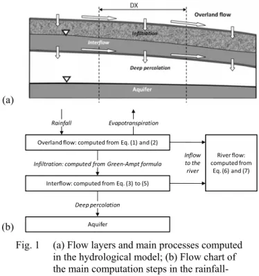
(2) Engineering Applications of Computational Fluid Mechanics Vol. 6, No. 1 (2012). falling on undrained areas has been discharged as overland flow. Rain falling on drained areas has been routed separately using a simplified modelling of the drainage network, called here virtual pipes. This separate modelling of the drained impervious areas constitutes our main original contribution.. surrounding areas (often considered as gardens) according to the local urban density (NRCS/ARS Curve Number Work Group and Moody, 2004). . In the model Topurban (Valeo and Moin, 2000), the runoff is routed separately depending on whether it is produced by pervious or impervious areas: rain falling on non saturated pervious areas is considered as throughflow, while runoff from impervious areas is considered as surface flow (with an optional routine accounting for storage ponds).. 2. RAINFALL-RUNOFF AND HYDRAULIC MODELS The rainfall-runoff model used here is processoriented and spatially distributed (Khuat Duy et al., 2010). Using a multi-layer approach based on layer-averaged equations (Figure 1), it computes the main hydrological processes, including overland flow, interflow, infiltration and deep percolation.. However, none of these approaches explicitly considers drainage systems, which may significantly modify the flow paths and shorten propagation times. Modelling the sewage systems is thus necessary if the rapidly-varying flows from drained impervious areas need to be represented. Detailed modelling of flows in drainage networks, such as sewers, is generally implemented only as far as urban hydrology is concerned. This refers to small-scale studies consisting mostly of impervious areas (Aronica and Cannarozzo, 2000; Rodriguez et al., 2008; Schmitt et al., 2004). In contrast, when broad-scale analyses of large watersheds are conducted, the impact of sewage systems is usually neglected, since most of the water travel time is spent in the river network. A watershed is considered here as “large” with respect to the impervious areas of interest, if the propagation time in the river network significantly exceeds the propagation time as overland flow in these impervious areas and to the river. In mid-size watersheds, the effect of the drainage network on discharge may not be negligible, while it may also not be feasible to take the drainage network into account with the same level of detail as in urban hydrology (Lhomme et al., 2004). In addition, the extent of drained areas remains hard to estimate (Walsh et al., 2009) and the opportunity of conducting direct measurements is restricted to limited cases mainly in urban hydrology (Alley and Veenhuis, 1983). In this paper, we present an original methodology to compute impervious surfaces accurately and to take drainage effects into account without modelling the entire drainage network in detail. An existing process-oriented and spatially distributed hydrological model has been adapted to accommodate the new methodology. The impervious surfaces have been estimated on the basis of landuse maps in vector format. Next, they have been classified as drained or undrained. Rain. (a) Rainfall. Evapotranspiration. Overland flow: computed from Eq. (1) and (2) Infiltration: computed from Green‐Ampt formula. Inflow to the river. River flow: computed from Eq. (6) and (7). Interflow: computed from Eq. (3) to (5) Deep percolation. (b). Aquifer. Fig. 1. (a) Flow layers and main processes computed in the hydrological model; (b) Flow chart of the main computation steps in the rainfallrunoff model.. The overland flow is modelled with the diffusive wave approximation. This model is derived from the fully dynamic shallow-water equations (SWE) by assuming that inertia terms may be neglected compared to gravity, friction and pressure terms. This assumption has been widely recognized as generally accurate for modelling overland flow (Jain and Singh, 2005). The hyperbolic fully dynamic shallow-water model may then be replaced by the following parabolic equation:. h   uh    vh    S with t x y h S fi  sin  i  cos  i i  x, y , i 47. (1).

(3) Engineering Applications of Computational Fluid Mechanics Vol. 6, No. 1 (2012). the infiltration coefficients, as suggested by Nearing et al. (1996). The rainfall runoff model computes lateral inflows to the rivers, which are next routed through the river network by means of the hydraulic model Wolf 1D. A suitable shock capturing scheme is used to solve the conservative form of the 1D Saint-Venant equations, enabling the simulation of flow regime changes and hydraulic jumps (Kerger et al., 2011). The following set of equations is solved:. where h [m] is the water depth, u and v [m/s] the velocity components along the x and y axis, S [m/s] the source terms (rainfall and infiltration), Sfi (i=x,y) [-] the friction slopes, θx [-] and θy [-] the projected bottom slopes. Using ManningStrickler formula, the velocity components can be related to the friction slopes as follows:. u. S fx 1 2/3 h 1/ 4 n  S 2fx  S 2fy . S fy 1 ; v  h 2/3 1/ 4 n  S 2fx  S 2fy . (2). . where n [s /m1/3] is a spatially distributed Manning coefficient. The infiltration is calculated using Green-Ampt formula (Chow et al., 1988), while the interflow is modelled with the depth-averaged Darcy equations. It is therefore computed using a diffusive wave equation similar to the overland flow equation:. p. hsub   usub hsub    vsub hsub     S sub t x y. usub  K s. vsub  K s. S. S. S fsub , x 2 fsub , x.  S 2fsub , y . 1/4. 2 fsub , x. . A. . (6) where A [m²] is the river cross section, q [m³/s] the discharge, h [m] the water height, qL [m³/s] the lateral inflow, J [-] the energy slope (accounting for bottom roughness and internal losses), θ [-] the mean bottom slope and lb [m] the channel bottom width. The pressure terms pA [m³] and px [m²] are defined as:. (3). (4). h. p A ( h)    h    l ( x,  ) d  ;.  S 2fsub, y . 1/ 4. S fsub ,i  sin  sub ,i  cos  sub ,i. .  qL      0    gA sin   gAJ  g cos  hl    hb   g cos  p  0  b x x  . ;. S fsub , x. q.   A     q2  t  q   x    g cos  p A . 0. hs i. h. i  x, y. p x ( h)    h   . (5). 0.  l ( x,  ) d x. (7). where l [m] is the channel width and a bound variable. The energy slope is evaluated using Manning formula as follows:. where p [-] is the soil effective porosity, hsub [m] the subsurface water depth, usub and vsub [m/s] the interflow velocity components, Ssub [m/s] the source terms (infiltration, deep percolation), Ks [m/s] the lateral hydraulic conductivity (spatially distributed), Sfsub,i (i=x,y) [-] the subsurface friction slopes, and θsub,i (i=x,y) [-] the projected slopes of the soil layer. Pre-processing of raw data has been carried out using the GIS interface of Wolf. The Digital Elevation Model (DEM) has been processed to remove depressions using an algorithm developed by Martz and Garbrecht (1999). The DEM-based flow paths have been made consistent with the real ones obtained from on-site surveys (Callow, 2007; Saunders, 1999). The roughness coefficient n has been deduced from landuse maps, while the soil type obtained from pedologic maps has been used to evaluate the soil conductivity based on pedotransfer functions (Rawls and Brakensiek, 1989). The influence of landuse on infiltration has been taken into account using effective values for. J. q2 K 2 A2 RH4/3. (8). with RH [m] the hydraulic radius and K [m1/3/s] the Strickler coefficient of the river. The spatial discretization of equations (1), (3) and (6) is based on the finite volume method combined with a self-developed flux-vector splitting technique. Upwind evaluation of the fluxes is performed, according to the sign of the flow velocity (Erpicum et al., 2010b). The stability of the scheme has been demonstrated using a linear stability analysis (e.g., Kerger et al., 2011). Efficiency, simplicity and low computational cost are the main advantages of this scheme. The resulting ordinary differential equations are integrated in time using an explicit Runge-Kutta scheme or an implicit algorithm based on the Generalized Minimal RESidual 48.

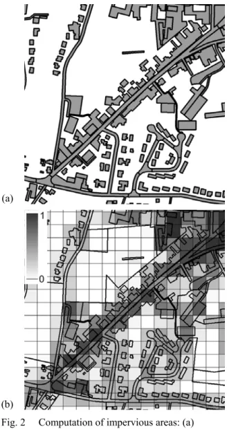
(4) Engineering Applications of Computational Fluid Mechanics Vol. 6, No. 1 (2012). method (GMRES). An original treatment of the junctions by means of Lagrange multipliers enables modelling of large river networks within a single simulation. The hydrologic inflows are treated as lateral inflows (source term qL) for the 1D simulations and have to be computed separately beforehand. The hydrologic and the river flow equations are therefore decoupled. The herein described models are parts of the modelling system Wolf, developed at the University of Liege. Wolf combines a set of complementary and interconnected modules for simulating free surface flows: process-oriented hydrology, 1D, 2D depth-averaged, 2D-vertical and 3D flow models. Their validity and efficiency have already been verified in numerous applications (Dewals et al., 2006; Dewals et al., 2008; Dufresne et al., 2011; Erpicum et al., 2009; Machiels et al., 2011), including inundation modelling (Dewals et al., 2011; Ernst et al., 2010; Erpicum et al., 2010a; Roger et al., 2009).. (a). 3. METHODOLOGY 3.1. Estimation of impervious surfaces. Existing methods to estimate the impervious surfaces can be classified as indirect or direct (Moglen, 2009). The former approach is the most standard one and consists in estimating the surface imperviousness based on the urban density, deduced from the corresponding landuse class, and using lookup tables (Beighley et al., 2009). This technique may however prove inaccurate, since the real amount of impervious areas for a given landuse class shows a high variability. Moreover, Thorndahl et al. (2006) highlighted that hydrological reduction factors calculated from measured rainfall and runoff have been found inconsistent with corresponding values for residential areas reported in literature. The indirect method is nonetheless often used, due to the wide data coverage available from remote sensing landuse recognition techniques. In contrast, direct methods identify the impervious areas by means of field surveys and aerial imagery, leading to a more accurate estimation of impervious surfaces (Beighley et al., 2009; Chabaeva et al., 2009; Jones and Jarnagin, 2009). The main drawbacks of direct methods are the limited availability and the cost of data. Endreny and Thomas (2009) introduced a combined approach, in which landuse maps were enhanced based on data on impervious areas extracted from road networks.. (b) Fig. 2. Computation of impervious areas: (a) Impervious landuse; (b) Impervious part of cells.. In our spatially distributed model, the impervious fraction of the surface has been computed in each cell based on landuse maps in vector format (Figure 2a). The impervious landuse types (such as roads, houses, car parks or concrete structures) have been selected and their corresponding surfaces have been summed for each cell, using a specific algorithm dedicated to the computation of overlay surface between a polygon and a regular mesh. As a result, a raster containing the impervious fraction of each cell has been obtained (Figure 2b). 3.2. Drainage network. After the computation of the impervious surface in each cell, drained and undrained cells have been distinguished. If data on the pipe network are available, our methodology assumes that all cells located within a given distance from the pipe network are drained. A cell is thus considered as 49.

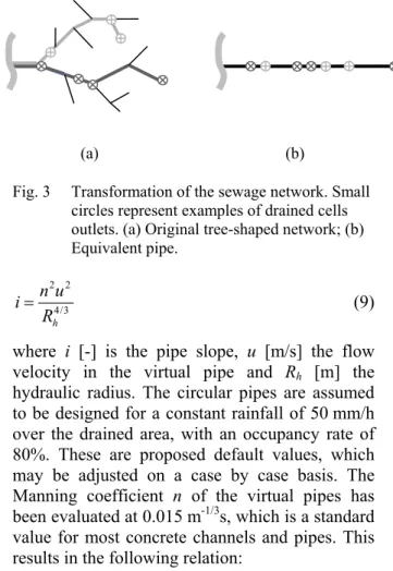
(5) Engineering Applications of Computational Fluid Mechanics Vol. 6, No. 1 (2012). drained if the distance from its centre to the nearest pipe is below a threshold value. The choice of this value is further analysed in the case study (section 4.2). In contrast, if the drainage network characteristics are unknown, the percentage of drained areas can be estimated following the approach suggested by Boyd (1993) for urban catchments. The estimation is based on selected low intensity rainfall events, during which the flow in the rivers is essentially generated from the drained impervious areas. The corresponding runoff coefficients are evaluated and their lower bound provides the part of drained areas in the catchment. This methodology applies provided a sufficiently high number of rainfall events are considered. Otherwise, the results may be affected by errors arising from measurement inaccuracies and from the selection of rainfall events during which not only drained impervious areas contribute to runoff. This method can also be used in combination with the previous one, either to validate the results or to calibrate the threshold distance from the drained areas to the pipe network. Real sewage systems are tree-shaped networks, with a high number of small pipes. The complete modelling of such systems for a whole watershed requires large amounts of data, usually partly unavailable. Moreover, the density of the network implies using very fine cells (down to a few meters) to represent the numerous individual pipes, reducing consequently the time step and dramatically increasing the computational cost. Our methodology consists in merging parts of this tree-shaped network into equivalent pipes, called hereafter virtual pipes, in order to reduce the model complexity while still representing the key processes leading to fast flow propagation to the river. As sketched in Figure 3, the runoff from each drained cell is discharged into a corresponding virtual pipe, at a location enabling to preserve the same length of flow path as in the real network. The slope of the virtual pipe is computed by a weighted average of the slopes of the corresponding real pipes. Its cross section varies as a function of the drained impervious surface. Since this cross-section depends on the detailed structure of the real network and on the dimensions of the real pipes, usually unknown, we have developed a relation to estimate default values for the equivalent pipe diameter. Uniform flow conditions are assumed in the pipe, as described by Manning-Strickler formula:. (a) Fig. 3. i. (b). Transformation of the sewage network. Small circles represent examples of drained cells outlets. (a) Original tree-shaped network; (b) Equivalent pipe.. n 2u 2 Rh4/3. (9). where i [-] is the pipe slope, u [m/s] the flow velocity in the virtual pipe and Rh [m] the hydraulic radius. The circular pipes are assumed to be designed for a constant rainfall of 50 mm/h over the drained area, with an occupancy rate of 80%. These are proposed default values, which may be adjusted on a case by case basis. The Manning coefficient n of the virtual pipes has been evaluated at 0.015 m-1/3s, which is a standard value for most concrete channels and pipes. This results in the following relation:.  Simp  Deq  0.005  1/2  i . 3/8. (10). where Deq [m] is the virtual pipe diameter, and Simp [m²] the impervious surface drained by the pipe. 3.3. River network. In a process-oriented and spatially distributed hydrological model, rivers serve as outlets for the runoff and baseflow, which are next propagated through the network of rivers. To this end, our methodology enables to determine the river network characteristics by combining three complementary data sources.. 50. . First, the DEM enables to generate a river network based on flow paths and a convergence treshold (Renssen and Knoop, 2000; Tarboton et al., 1991). This network covers the whole watershed, but contains limited information on the cross-sectional geometry of the rivers.. . Second, data from field surveys are exploited to incorporate a more detailed description of the river geometry and cross sections. However, such detailed data are generally available only on a limited part of the basin..

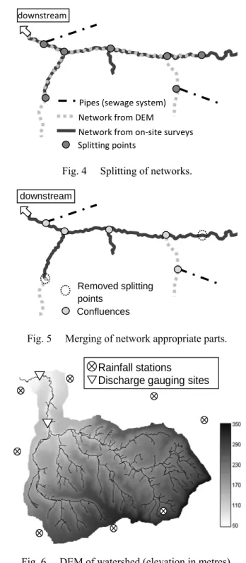
(6) Engineering Applications of Computational Fluid Mechanics Vol. 6, No. 1 (2012). . A third source of data is obtained from the sewage network, generated using the method described in section 3.2.. downstream. The overall procedure for generating the river network involves the following six steps: . The DEM is first modified using a dedicated algorithm to force the topography-based river paths to follow the real river courses where such data are available. Engineering structures affecting the flowpaths (such as road or railway dikes) are taken into account at this stage of the procedure.. . Next, a first river network is generated based on this modified DEM.. . In parallel, a second network is created using the field survey data, including every relevant hydraulic structure such as culverts, footbridges and pipes.. . Finally, these two networks and the additional pipes from the sewage system are merged. This is performed in three sub-steps:. Pipes (sewage system) Network from DEM Network from on‐site surveys Splitting points . Fig. 4. Splitting of networks.. downstream. Removed splitting points Confluences. 1. The river branches are first split into multiple reaches between characteristic points, such as junctions (Figure 4). Fig. 5. Merging of network appropriate parts.. Rainfall stations Discharge gauging sites. 2. Next, the DEM-based river reaches are replaced by field survey-based reaches where these are available. Possible inconsistencies between both networks, such as bed level discontinuities at the junctions, are handled at this stage of the process. 3. Eventually, all river reaches are merged again to form the complete river network (Figure 5). This method automatically generates a 1D network, which (i) covers the whole watershed, (ii) includes detailed data from field surveys (including cross sections and hydraulic structures, such as weirs and culverts) and (iii) incorporates the virtual pipes representing the drainage network.. Fig. 6. 4.1. DEM of watershed (elevation in metres).. Watershed description. The watershed is mainly covered by meadows (70%) and includes several low or mediumdensity towns. The DEM of the watershed is characterized by a mean slope of 7.2% (Figure 6). Hourly discharge measurements are provided by two gauging stations located on the river, while rainfall is measured daily at eight stations and hourly at one station. These stations are located either inside or nearby the catchment. A disagregation process has been applied to the daily series to provide hourly rainfall intensities (Koutsoyiannis, 1994; Koutsoyiannis, 2003).. 4. CASE STUDY. The methodology has been applied to the Berwinne watershed located in Belgium. River Berwinne is a tributary of river Meuse and has a catchment area of 132 km².. 51.

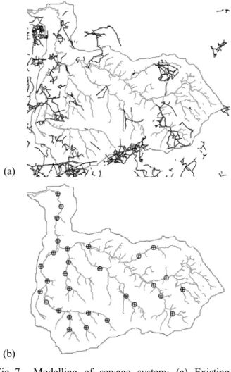
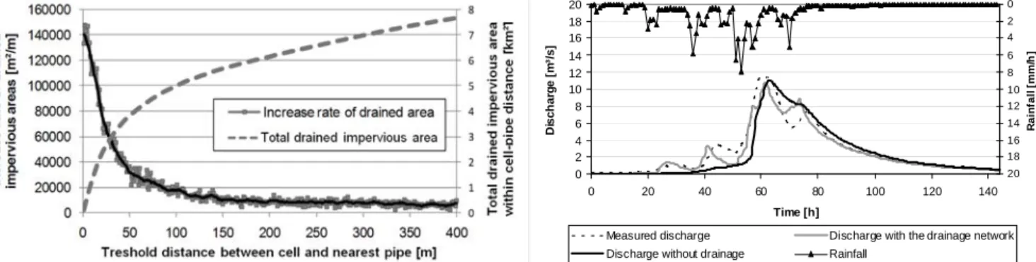
(7) Engineering Applications of Computational Fluid Mechanics Vol. 6, No. 1 (2012). 4.2. Application of the methodology. According to the procedure described above, the impervious surfaces have been computed based on landuse maps (section 3.1). These landuse maps were available in vector format on 92% of the watershed (source: Belgian National Geographic Institute). Application of this method has resulted in a mean value of 6.3% of impervious surfaces throughout the watershed. Modelling of the drained impervious areas has been performed based on the real sewer system, provided in the “Plan d'Assainissement par Sousbassin Hydrographique (PASH)” (SPGE 2007). These maps include the coordinates of the existing pipes in vector format (Figure 7a). Using the method described in section 3.2, the sewage network trees have been merged into virtual pipes. Virtual pipes with nearby outlets have been combined in order to further reduce the total number of pipes directly connected to the river. To obtain a reasonable number of virtual pipes in the final network, a minimal distance of 1000 m between two adjacent outlets was imposed. With this value, the propagation time lag between two adjacent outlets remains far below the time step at which rainfall data is available. Applying this methodology has resulted in a set of 30 virtual pipes representing the entire drainage network. The virtual pipes can be represented in the network by arbitrary lines of adequate length and starting from their outlet point situated along the river (Figure 7b). The cells are considered as drained by the sewage system if their centre lies at a distance below 150 m from the pipes. This distance represents the runoff path on impervious surfaces, in the gutters and in small pipes which do not appear in the drainage network. A sensitivity analysis has been carried out to assess the influence of this parameter on the drained surface. To this end, the distance from each cell to the nearest pipe was first computed (Figure 8). Using this information in the part of the map covered by vector data, the total drained impervious surface (sum of impervious areas from drained cells) has next been plotted as a function of the cell-pipe distance threshold (Figure 9). For small values of threshold distance from cell to pipe (below 50 m), the surface of drained impervious areas is found to increase significantly with the threshold value. This results from the tree-shape of the network. As can be seen in Figure 8, the chosen distance (150 m) enables to consider as drained most urbanized areas located. (a). (b) Fig. 7. Modelling of sewage system: (a) Existing sewage network; (b) Locations of outlets of virtual pipes.. Fig. 8. Distance (in metres) from each cell to nearest pipe (zoom on a town located in watershed).. near the sewage network. Above this distance, the rate of increase of the drained area with the threshold distance becomes significantly lower (Figure 9). This residual increase rate corresponds to the impervious areas located outside urbanized areas, such as roads or isolated houses and structures. 52.

(8) 20 18 16. 0. 14 12 10 8 6 4 2 0. 6. 2 4 8 10 12 14. Rainfall [mm/h]. Discharge [m³/s]. Engineering Applications of Computational Fluid Mechanics Vol. 6, No. 1 (2012). 16 18 20. 0. 20. 40. 60. 80. 100. 120. 140. Time [h]. Fig. 9. Drained impervious area and rate of change of drained impervious area (with moving average) as a function of the cell-pipe distance.. Measured discharge. Discharge with the drainage network. Discharge without drainage. Rainfall. Fig. 11 August 1996 flood: Rainfall intensity and comparison between measured and computed discharge at downstream gauging station.. 4.3. Validation. To assess the benefits of modelling the drainage network, simulations have been conducted for a real rainfall event (August 2006). Results obtained both with and without modelling of the drainage network have been compared with measured discharges at the most downstream gauging station. In both cases, the considered total impervious area was the same. Hourly rainfall values, disaggregated from daily values at the weather stations, were distributed over the catchment using the Thiessen polygons method. The program MudRain developed by Koutsoyiannis (2003) was used to perform multivariate disaggregation of rainfall data. Since the considered rainfall event occurred during a low-flow period, the baseflow has been shown to be negligible compared to the subsequent flood discharge. For the simulation without consideration of the drainage network, the spatially-distributed friction coefficient and soil conductivity were calibrated manually. The default parameter values, which were deduced from landuse maps and pedologic maps, have been multiplied by a different coefficient depending on the landuse category and soil type. In Figure 11, the rainfall intensities are plotted as spatially weighted means, while the dotted line represents the measured hydrograph at the gauging station. Measurement uncertainty is limited since the gauging curve has been extrapolated for high discharges using local 2D hydraulic modelling, instead of a mathematical extrapolation. Modelling the drainage network adds a fast flow component, which significantly modifies the computed hydrograph. This leads to a better representation of the observed flow rates, since the fast flow component is indeed similar to the. Fig. 10 Analysis of rainfall-runoff values for low intensity events.. In the Berwinne watershed, the computed drained impervious area was found to cover 2.5% of the catchment surface. A complementary analysis of discharge measurements from low intensity rainfall events has been carried out to estimate the drained impervious areas, as detailed in section 3.1. Figure 10 shows a rainfall-runoff plot, in which the baseflow component was subtracted from the measured discharge. All rainfall events considered in this analysis took place during lowflow periods, for which the baseflow was found almost constant and below 0.5 m³/s. The line shows a runoff coefficient of 2.1%. Most measured coefficients are bounded by this minimum value. This is a lower bound, since rainfall events during which undrained areas contributed to the runoff production have a higher runoff to rainfall ratio. This suggests that the drained impervious areas produce about 2.1% of the total runoff. Considering a mean runoff coefficient of 0.85 for these areas, to account for losses (evapotranspiration, surface storage), the impervious surface of the catchment is therefore estimated at 2.1% / 0.85 = 2.5% of its total surface. This value is fully consistent with the value estimated previously on the basis of the landuse map and the drainage network. 53.

(9) Engineering Applications of Computational Fluid Mechanics Vol. 6, No. 1 (2012). measurements. In contrast, the model disregarding drainage failed to represent the first peaks, since the runoff production from impervious areas does not reach the river fast enough to produce the first peak. For this event, the Nash-Sutcliffe efficiency coefficient has been found to improve from 0.81 to 0.92 (Nash and Sutcliffe, 1970). Nevertheless, some differences remain between the two curves. Although runoff on drained areas generates a rapidly varying flow component, other processes also influence the discharge at an hourly time steps. For instance, saturated areas located close to the river may similarly induce rapidly varying flows (Cosandey, 1996). The disaggregation of daily rainfall to hourly series is another source of uncertainty.. predictions, but may not be considered as the only phenomenon determining the rapidly varying flow components of river hydrographs. The proposed methodology constitutes an original approach for the modelling of drained areas. The proposed simplified modelling of the drainage network can be usefully incorporated into existing rainfall-runoff models and can be run automatically, requiring limited extra effort from the modeller. Further verification using additional rainfall events and different catchments is still needed to assess more generally the performance of the methodology and the sensitivity of the results. In future developments of the concept of virtual pipes, the main original contribution of the present research, the focus should be set on the sizing of the pipes, in order to compute more accurately the flow propagation through the real network. Additionally, it would be of key practical interest to identify objective criteria to assess a priori the need for explicitly modelling the drainage network, based on the watershed size and its mean degree of urbanisation.. 5. CONCLUSIONS. Impervious surfaces can produce a significant part of the surface runoff. In small and mid-size watersheds, the flow dynamics of the water falling on such impervious areas differs significantly depending on whether these areas are connected or not to a drainage network, such as a sewage system. A methodology has been developed to accurately compute the contributions of impervious surfaces and to take into account the main effects of the drainage network without the need for its detailed modelling. The impervious part of each cell surface is computed as the sum of the impervious areas delimited in a detailed landuse map in vector format. The real drainage network is modelled by means of a simplified network, called virtual pipes, which routes the rain falling on drained cells to the river. The separation of drained and undrained areas is based on a maximal distance criterion between the cells and the nearest pipe from the drainage network. In the case study of river Berwinne, the model not taking into account the drainage network failed to simulate the fast evolution of the river discharges, even after a calibration process. In contrast, the improved capacity of the developed model to represent the river dynamics at an hourly time step has been demonstrated in this case study. Nevertheless, the computed river discharges at such small time scales may also be affected by other hydrological processes (e.g. rainfall falling on saturated areas near the rivers) and by uncertainties due to data resolution (e.g. daily rainfall time series disaggregated into hourly series). Therefore, accounting for the drained impervious areas is necessary to improve flow. NOMENCLATURE. A Deq h hsub i J K Ks l lb n pω, px q qL. Rh S Sfi Sfsub,i Simp 54. river cross section [m²] equivalent pipe diameter [m] water depth [m] subsurface water dept [m] slope of virtual pipe energy slope (accounting for bottom roughness and internal losses) Strickler coefficient of the river [m1/3/s] lateral hydraulic conductivity [m/s] channel width [m] channel bottom width [m] Manning coefficient [s /m1/3] pressure terms defined in (7) [m³] [m²] discharge [m³/s] lateral exchanges (lateral inflow and exchanges between mainstream and floodplains) [m³/s] the hydraulic radius [m] source terms (rainfall and infiltration) [m/s] friction slopes (i=x,y) subsurface friction slopes (i=x,y) impervious surface drained by a.

(10) Engineering Applications of Computational Fluid Mechanics Vol. 6, No. 1 (2012). Ssub u, v usub, vsub θ θsub,i θx, θy. virtual pipe [m²] source terms (infiltration, deep percolation) [m/s] velocity components along x and y axis [m/s] interflow velocity components [m/s] mean bottom slope projected slopes of the soil layer (i=x,y) projected bottom slopes. 11. 12.. 13.. REFERENCES. 14.. 1. Alley WM, Veenhuis JE (1983). Effective impervious area in urban runoff modeling. Journal of Hydraulic Engineering 109(2):313-319. 2. Aronica G, Cannarozzo M (2000). Studying the hydrological response of urban catchments using a semi-distributed linear non-linear model. Journal of Hydrology 238(1-2):35-43. 3. Beighley E, Kargar M, He Y (2009). Effects of impervious area estimation methods on simulated peak discharges. Journal of Hydrologic Engineering 14(4):388-398. 4. Boyd MJ (1993). Pervious and impervious runoff in urban catchments. Hydrological Sciences Journal 38(6):463-478. 5. Brabec EA (2009). Imperviousness and landuse policy: Toward an effective approach to watershed planning. Journal of Hydrologic Engineering 14(4):425-433. 6. Callow JN (2007). How does modyfying a DEM to reflect known hydrology affect subsequent terrain analysis? Journal of Hydrology 332:30-39. 7. Chabaeva A, Civco DL, Hurd JD (2009). Assessment of impervious surface estimation techniques. Journal of Hydrologic Engineering 14(4):377-387. 8. Chau KW, Wu CL, Li YS (2005). Comparison of several flood forecasting models in Yangtze River. Journal of Hydrologic Engineering 10:485. 9. Cheng CT, Ou CP, Chau KW (2002). Combining a fuzzy optimal model with a genetic algorithm to solve multi-objective rainfall-runoff model calibration. Journal of Hydrology 268(1-4):72-86. 10. Cheng CT, Wang WC, Xu DM, Chau KW (2008). Optimizing hydropower reservoir operation using hybrid genetic algorithm and. 15.. 16.. 17.. 18.. 19.. 20.. 21.. 22.. 55. chaos. Water Resources Management 22(7):895-909. Chow VT, Maidment D, Mays LW (1988). Applied Hydrology. McGraw-Hill. Cosandey C (1996). Surfaces saturées, surfaces contributives : Localisation et extension dans l'espace du bassin versant. Hydrological Sciences Journal 41(5):751-761. Dewals BJ, Erpicum S, Archambeau P, Detrembleur S, Pirotton M (2006). Depthintegrated flow modelling taking into account bottom curvature. J. Hydraul. Res. 44(6):787795. Dewals BJ, Kantoush SA, Erpicum S, Pirotton M, Schleiss AJ (2008). Experimental and numerical analysis of flow instabilities in rectangular shallow basins. Environ. Fluid Mech. 8:31-54. Dewals BJ, Erpicum S, Detrembleur S, Archambeau P, Pirotton M (2011). Failure of dams arranged in series or in complex. Natural Hazards 56(3):917-939. Dufresne M, Dewals BJ, Erpicum S, Archambeau P, Pirotton M (2011). Numerical investigation of flow patterns in rectangular shallow reservoirs. Engineering Applications of Computational Fluid Mechanics 5(2):247258. Endreny TA, Thomas KE (2009). Improving estimates of simulated runoff quality and quantity using road-enhanced land cover data. Journal of Hydrologic Engineering 14(4):346-351. Ernst J, Dewals BJ, Detrembleur S, Archambeau P, Erpicum S, Pirotton M (2010). Micro-scale flood risk analysis based on detailed 2D hydraulic modelling and high resolution land use data. Nat. Hazards 55(2):181-209. Erpicum S, Meile T, Dewals BJ, Pirotton M, Schleiss AJ (2009). 2D numerical flow modeling in a macro-rough channel. Int. J. Numer. Methods Fluids 61(11):1227-1246. Erpicum S, Dewals BJ, Archambeau P, Detrembleur S, Pirotton M (2010a). Detailed inundation modelling using high resolution DEMs. Engineering Applications of Computational Fluid Mechanics 4(2):196-208. Erpicum S, Dewals BJ, Archambeau P, Pirotton M (2010b). Dam-break flow computation based on an efficient flux-vector splitting. Journal of Computational and Applied Mathematics 234(7):2143-2151. Fleming G (1975). Computer Simulation Techniques in Hydrology. American Elsevier Publishing Co., Inc..

(11) Engineering Applications of Computational Fluid Mechanics Vol. 6, No. 1 (2012). 35. Mcmillan HK, Brasington J (2008). End-toend risk assessment: A coupled model cascade with uncertainty estimation. Water Resources Research 44(W03419):14. 36. Moglen GE (2009). Hydrology and impervious areas. Journal of Hydrologic Engineering 14(4):303-304. 37. Nash JE, Sutcliffe JV (1970). River flow forecasting through conceptual models part I A discussion of principles. Journal of Hydrology 10(3):282-290. 38. Nearing MA, Liu BY, Risse LM, Zhang X (1996). Curve numbers and Green-Ampt effective hydraulic conductivities. Water Resources Bulletin 32(1). 39. NRCS/ARS Curve Number Work Group, Moody HF (2004). Hydrologic soil-cover complexes. In: Part 630 Hydrology National Engineering Handbook. Ed. USDA. 40. Rawls WJ, Brakensiek DL (1989). Estimation of soil water retention and hydraulic properties. In: Unsaturated Flow in Hydrologic Modeling. Ed. Morel-Seytoux HJ. Kluwer Academic Publishers. 41. Renssen H, Knoop JM (2000). Global river routing network for use in hydrological modeling. Journal of Hydrology 230(34):230-243. 42. Rodriguez F, Andrieu H, Morena F (2008). A distributed hydrological model for urbanized areas - Model development and application to case studies. Journal of Hydrology 351(34):268-287. 43. Roger S, Dewals BJ, Erpicum S, Schwanenberg D, Schüttrumpf H, Köngeter J, Pirotton M (2009). Experimental und numerical investigations of dike-break induced flows. J. Hydraul. Res. 47(3):349359. 44. Saunders W (1999). Preparation of DEMs for use in environmental modelling analysis. 1999 ESRI User Conference, San Diego, California. 45. Schmitt TG, Thomas M, Ettrich N (2004). Analysis and modeling of flooding in urban drainage systems. Journal of Hydrology 299(3-4):300-311. 46. SPGE (2007). Plans d'Assainissement par Sous-bassins Hydrographiques - document de travail - : mise à jour juin 2007. 47. Tarboton DG, Bras RL, Rodriguez-Iturbe I (1991). On the extraction of channel networks from digital elevation data. Hydrological Processes 5(1):81-100. 48. Thorndahl S, Johansen C, Schaarup-Jensen K (2006). Assessment of runoff contributing. 23. Garen DC, Moore DS (2005). Curve number hydrology in water quality modeling: uses, abuses, and future directions. Journal of the American Water Resources Association 41(2):377-388. 24. Hjelmfelt AT, NRCS/ARS Curve Number Work Group, Moody HF (2004). Estimation of direct runoff from storm rainfall. In: Part 630 Hydrology National Engineering Handbook. Ed. USDA. 25. Jain MK, Singh VP (2005). DEM-based modelling of surface runoff using diffusion wave equation. Journal of Hydrology 302(14):107-126. 26. Jones JW, Jarnagin T (2009). Evaluation of a moderate resolution, satellite-based impervious surface map using an independent, high-resolution validation data set. Journal of Hydrologic Engineering 14(4):369-376. 27. Kerger F, Archambeau P, Erpicum S, Dewals BJ, Pirotton M (2011). A fast universal solver for 1D continuous and discontinuous steady flows in rivers and pipes. Int. J. Numer. Methods Fluids 66:38-48. 28. Khuat Duy B, Archambeau P, Dewals BJ, Erpicum S, Pirotton M (2010). River modelling and flood mitigation in a Belgian catchment. Proc. Inst. Civil. Eng.-Water Manag. 163(8):417-423. 29. Koutsoyiannis D (1994). A stochastic disaggregation method for design storm and flood synthesis. Journal of Hydrology 156(14):193-225. D (2003). Rainfall 30. Koutsoyiannis disaggregation methods: Theory and applications. In: Workshop on Statistical and Mathematical Methods for Hydrological Analysis, Rome. 31. Lhomme J, Bouvier C, Perrin JL (2004). Applying a GIS-based geomorphological routing model in urban catchments. Journal of Hydrology 299(3-4):203-216. 32. Lin JY, Cheng CT, Chau KW (2006). Using support vector machines for long-term discharge prediction. Hydrological Sciences Journal 51(4):599-612. 33. Machiels O, Erpicum S, Archambeau P, Dewals BJ, Pirotton M (2011). Theoretical and numerical analysis of the influence of the bottom friction formulation in free surface flow modeling. Water SA 37(2):221-228. 34. Martz LW, Garbrecht J (1999). An outlet breaching algorithm for the treatment of closed depressions in a raster DEM. Computers & Geosciences 25:835-844.. 56.

(12) Engineering Applications of Computational Fluid Mechanics Vol. 6, No. 1 (2012). 49. 50.. 51.. 52.. catchment areas in rainfall runoff modelling. Water Science & Technology 54(6-7):59-56. Valeo C, Moin SMA (2000). Variable source area modelling in urbanizing watersheds. Journal of Hydrology 228(1-2):68-81. Walsh CJ, Fletcher TD, Ladson AR (2009). Retention capacity: A metric to link stream ecology and storm-water management. Journal of Hydrologic Engineering 14(4):399-406. Wang WC, Chau KW, Cheng CT, Qiu L (2009). A comparison of performance of several artificial intelligence methods for forecasting monthly discharge time series. Journal of Hydrology 374(3-4):294-306. Wu CL, Chau KW, Li YS (2009). Predicting monthly streamflow using data-driven models coupled with data-preprocessing techniques. Water Resources Research 45(8).. 57.

(13)