May 19 -24, 2013, Orlando, Florida, USA
Comparison of parameterization schemes for solving the discrete material optimization
problem of composite structures
Pierre Duysinx1, Maria Guillermo1, Tong Gao2, Michael Bruyneel3
1
University of Liege (Ulg), Belgium, {p.duysinx, mguillermo}@ulg.ac.be
2 Northwestern Polytechnical University (NWPU), Xi’an, China, [email protected] 3
LMS-SAMTECH, Belgium, [email protected]
1. Abstract
Optimal design of composite structures can be formulated as an optimal selection of material in a list of different laminates. Based on the seminal work by Stegmann and Lund, the optimal problem can be stated as a topology optimization problem with multiple materials. The research work carries out a large investigation of different interpolation and penalization schemes for the optimal material selection problem. Besides the classical Design Material Optimization (DMO) scheme and the recent Shape Function with Penalization (SFP) scheme by Bruyneel, the research introduces a generalization of the SFP approach using a bi-value coding parameterization (BCP) by Gao, Zhang and Duysinx. The paper provides a comparison of the different parameterization approaches. It also proposes alternative penalization schemes and it investigates the effect of the power penalization. Finally, we discuss the solution aspects in the perspective of solving large-scale industrial applications. The conclusions are illustrated by a numerical application for the compliance maximization of an in-plane composite ply.
2. Keywords: Composite Structure Optimization, Topology Optimization, Discrete Material Optimization Sequential Convex Programming.
3. Introduction
Taking the best of composite material high strength and stiffness to weight ratios is essential to improve the efficiency of airplanes, ground vehicles, wind turbines and renewable energy systems. To this end, the discrete optimal orientation optimization is a fundamental problem of composite structure optimization, which can be applied to solve different problems of interest, for instance, the optimal orientation distribution problem of plies, or the optimal stacking sequence of multiple-layer laminated structures. The Discrete Material Optimization (DMO) approach proposed by Stegmann and Lund [10] has opened a breakthrough in composite optimization. The fundamental idea is to formulate the composite optimization problem as an optimal material selection problem in which the different laminates and ply orientations are considered as different materials and to solve it as a topology optimization problem using continuous variables.
This approach can be regarded as a generalization of the multi-phase topology optimization proposed in Thomsen [12] and in Sigmund and Torquato [9]. To transform the discrete problem into a continuous one, one introduces a suitable parameterization to express the material properties as a weighted sum of the candidate material properties. Some difficulties of the discrete material selection using topology optimization are 1/ to find efficient interpolation and penalization schemes of the material properties and 2/ to be able to have efficient solution algorithms to handle very large scale optimization problems with many design variables. Besides the seminal work by Stegmann and Lund [10], we extend and generalize the work by Bruyneel [2] with the alternative SFP scheme by using a bi-value coding parameterization (BCP) by Gao et al. [6]. The present research work carries out a large investigation of different interpolation and penalization schemes for the optimal material selection problem. In particular, the work considers the solution aspects in the perspective of solving large-scale industrial applications.
4. Discrete Material Optimization Models
The discrete optimal orientation design of the laminate can be treated as an optimization material selection problem with multiple materials. Following the idea by Lund and Stegmann [10], the Discrete Material Optimization (DMO) consists in writing the linear anisotropic material stiffness matrix Ci of a composite ply noted
‘i’ as a weighted sum over the stiffness of some candidate materials {j} (i.e. plies with different orientations):
m j i
wij i
1 0 ij 1 ij 1 ik 0 when ij 1 j w w w k j w
(2)From the conditions (2), it comes that no additional constraint is needed to ensure the presence of a single material phase at each design element if one end up with a 0/1 design satisfying the constraints. This is achieved by using a penalization of the intermediate densities
4.1. Discrete Material Optimization (DMO)
Stegmann and Lund [10] presented several Design Material Optimization (DMO) interpolation schemes, among which the most usual one (usually called DMO4) is:
v 1 1 with 0 1 m p p ij ij i ij j w x x x
(3)In this scheme, the number of design variables attached to each designable element or region just equals the number of candidate material phase, i.e., mv=m. The design variables range from 0 to 1, meaning the presence or
absence of material i. As in the SIMP method, the penalization factor p is applied to push the design variables to their extreme values 0 and 1.
4.2. Shape Function with Penalization
More recently, Bruyneel [2] presented an alternative parameterization model named SFP based on the finite element shape functions. For a design problem with 0°, 90°, -45° and 45° plies, the shape functions of four-node finite elements are introduced as:
1 1 2 2 1 2 3 1 2 4 1 2 1 1 1 1 1 1 4 4 1 1 1 1 1 1 4 4 1 1, 1, 2,3, 4 p p i i i i i i p p i i i i i i ij w x x w x x w x x w x x x j (4)Obviously, the SFP interpolation scheme also satisfies the conditions (2). As in the SIMP method, the penalization factor p is applied to push the design variables to their extreme values +/-1. When compared to the DMO scheme, SFP introduces only two variables for four fiber orientations. In SFP, the presence of one material phase is characterized by a specific combination of design variables taking bi-values of +1 and/or -1. The smaller number of design variables in SFP is an advantage over the DMO schemes to reduce the size of the optimization problem. As indicated in Ref. [2], even if it may be quite difficult, it is possible, in principle, to extend the SFP to more than four materials by building complex shape functions related to ‘n’ node finite elements satisfying the conditions (2). 4.3. Bi-value coding parameterization (BCP)
The bi-valued coding parameterization (BCP) scheme generalizes the SFP scheme and provides an alternative to the classical DMO interpolation scheme. To overcome the shortcoming of the SFP scheme, one can abandon the idea of finite element shape functions and keep in mind only the idea of defining the shape function using bi-values of +1 and -1. Thus, a new BCP scheme is proposed here as the material parameterization model for ‘m’ material phases,
v v 1 1 1 with 1 1 and 1, , 2 v p m i j m jk ik ik k w s x x k m
(5)where mv, the number of design variables is an integer defined by the ceiling function of mv=log2m. In other words,
the BCP scheme makes it possible to interpolate between 2(mv1)1 and 2mv material phases with m
v design
variables. For example, for mv=3 one can interpolate between m materials with 5≤m≤8. The sjk values are given at
Tables 1 and 2 for 2 and 3 binary coding variables. The values of sjk are equal to 1 or -1. For mv=2 obviously the
BCP material parameterization recovers exactly the SFP scheme (4). To illustrate the “coding” clearly, a sketch is shown in Fig. 1. Each candidate material phase locates at the vertex of the square or of a cube in the 2D or 3D spaces.
Table 1:
s
jkvalues (mv=2, m=4) j k 1 2 3 4 1 -1 1 1 -1 2 -1 -1 1 1 Table 2:s
jkvalues (mv=3, m=8) j k 1 2 3 4 5 6 7 8 1 -1 1 1 -1 -1 1 1 -1 2 -1 -1 1 1 1 1 -1 -1 3 -1 -1 -1 -1 1 1 1 1 M1 M2 M3 M4 1 x 2 x -1 -1 1 1 1 x 2 x 3 x M1 M2 M3 M4 M5 M6 M7 M8 (a) mv=2, m=4 (b) mv=3, m=8Figure 1: Illustrations of the BCP scheme 4.3. Penalization of intermediate densities
In eq. (3), (4) and (5), the power penalization of intermediate is used to prevent the intermediate values of the design variables at the solution, and therefore to avoid any mixture of candidate materials in the final design. The power penalization with an exponent p [1] is very convenient but this choice is not unique. Other penalization schemes have been explored successfully by the authors: If the intermediate values of a variable must be penalized, the following schemes have been investigated:
-SIMP [1] ( ) p f (6) -RAMP [11] ( ) 1 (1 ) f p (7) -Halpin Tsai [7] ( ) (1 ) r f r (8) -Polynomial [13] 1 1 ( ) p f (9)
Basically, one can find equivalent penalizations of intermediate densities by a proper choice of the penalization parameter in each scheme. For instance, the parameters p = 3 for SIMP, r = 0.269 for Halpin-Tsai and = 16 for the polynomial scheme provide similar penalization schemes. Our numerical experiments showed that the different
The authors also investigated continuation procedures in which the penalization is progressively increased. Because of the presence of many local optima, the idea is to use a classic continuation strategy to increase progressively the penalization parameter. However, the continuation strategy gives no guarantee to avoid the local optima. It is just reduces the tendency to be trapped in a local configuration.
5. Laminate stiffness optimization problem 5.1. Minimization of structural compliance
Here, the minimum compliance design of a laminated composite is considered with fiber angles to be optimized. With a discrete material parameterization, the optimization problem of a laminate can be stated as follows:
v
T find: 1, , ; 1, , minimize: subject to: ik x i n k m C F u F Ku (10)One notices that no volume constraint is included because we consider an optimum orientation problem. For fixed loads, the sensitivity of the compliance can be generally expressed as:
T T T 2 ik ik ik ik C x x x x F K K u u u u u (11)
For each finite element, the element stiffness matrix is calculated using one of the interpolation schemes (3), (4) or (5) so that the partial derivative can be calculated with:
1 m ij j i i j ik ik w x x
K K (12)Obviously, from the sensitivity expression, the sensitivity C/xik might be positive or negative due to the
summation expression of the stiffness interpolation scheme, which means the objective function can be non-monotonous and many local solutions might exist. The large-scale optimization problem is solved by applying the well-known concept of sequential convex programming (SCP), in which one resorts to a sequence of convex subproblems of (10). In this paper, the structural analysis is carried out using SAMCEF finite element software and the MMA family optimizer [4] is adopted to seek the optimal solution of each subproblem.
5.2. Maximization of natural frequency
The problem of maximization of natural frequency is stated as follows:
v 2 2 find: 1, , ; 1, , minimize: subject to: 0 1 1 ik ik x i n k m x K M u (13)where K and M are the stiffness and mass matrix of the whole structure, respectively. ω is one of the circular natural frequencies and u the corresponding mode shape. Likewise, the sensitivities can be derived by differentiating the eigenvalue equation so that
T 2 T 2 T i i i i i i ik ik ik x x x K M u u u u u Mu (14)
where Mi is the element mass matrix. Generally, the natural frequency is a non-monotonous function of design
variables because the sensitivity in eq. (14) might be positive or negative. Here, it is important to notice that both element stiffness and mass matrices should be parameterized. Similarly to the situation of stiffness matrix, the mass matrix can be written as follows if using for instance the BCP interpolation scheme:
v
v 1 1 1 1 2 M p m m j i ij i i j m ik ik j k v v s x
M M (15)Notice that the penalty factors pK and pM in both interpolations may take different values. However generally one
5.3. Introduction of a volume constraint
In fact, the BCP scheme presented above can only be used to attribute a certain solid material phase of all candidates to each finite element while no void is allowed. To reduce the structural weight, the following interpolation model was proposed by Bruyneel et al. [5] to allow the selection of discrete materials and the presence of void simultaneously.
1 0 1 m j q i i ij i i j c y w c y
(16)where yi refers to the additional topology variable that identifies the presence of the solid material
(yi=1;wij=1;wik=0, k≠ j) and void (yi=0) over element i. q is the penalization factor intending to push yi toward 0 or
1. Correspondingly, the volume constraint can be stated as i i i
V
y V V (17)Here, V denotes the whole volume of the structure accumulated by each element volume Vi full of solid materials.
V refers to the upper bound of the volume constraint. Note that the volume is controlled without distinction
between solid material phases.
However, if the volume constraint is concerned with specific material phases for a general layout design of inhomogeneous materials, the above expression is no longer suitable. Suppose ξ and ζ indicate two different sets of solid material phases, e.g., porous materials and fiber reinforced composites, the following parameterization model of general form is proposed to distinguish the contributions of specific material phases
1 0 1 q q i i i i i i i i c y w c y w c y
(18)In this case, the volume control of material set ξ still holds the expression of eq. (14). Clearly, the parameterization model of eq. (18) will automatically degenerate into eq. (16) if only one set of solid material phase exists. To guarantee the “uniform” weights, i.e. exactly “fair” starting guess of each candidate material, the initial value of the topology variable should be set to be yi=0.5
1/q
, depending upon the penalization factor q. An alternative general interpolation model using the “
1
bi-value” concept is written as: 1 1 1 1 2 2 q q i i i i i i i i y y c w c w c y
(19)Correspondingly, the volume constraint used to control material set ξ is expressed as 1 1 1 2 i i i i y V V V y
(20)In fact, material set ζ is indirectly controlled when the volume constraint is imposed to material set ξ. Likewise, a “uniform” weighting can be achieved when the initial value is set to be yi=0.
6. Numerical applications
In this section, we consider several numerical applications to illustrate and compare the different interpolation schemes.
6.1. Structural compliance minimization
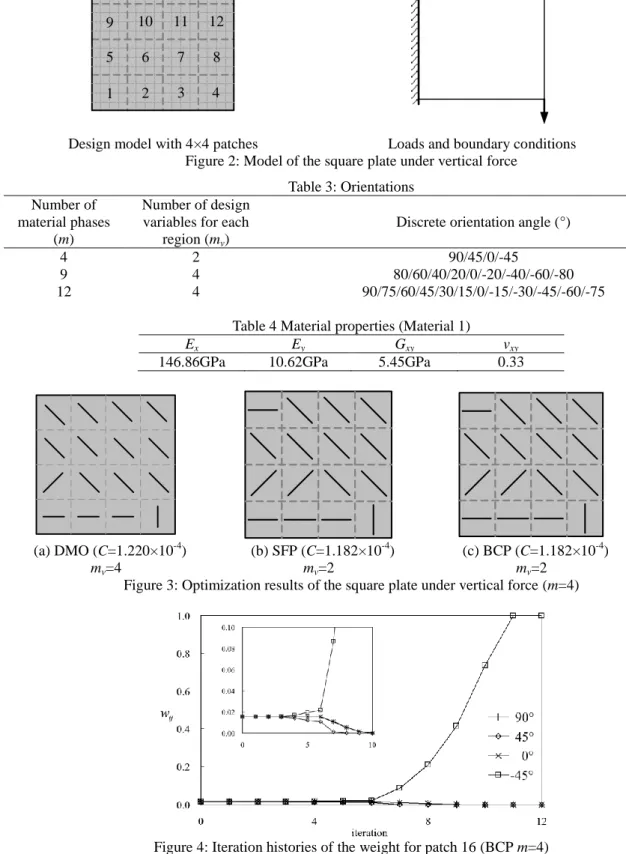
The maximum in-plane compliance problem (10) is solved by selecting the optimal orientation of the ply. An orthotropic composite material whose properties are listed in Table 4. The local ply orientation can be searched in a list of discrete orientation angles (see Table 3). A square structural domain consisting of a single ply is considered (see Fig. 2). The model is meshed with 16×16 quadrangular finite elements. The structure is clamped along the left edge and a pin point vertical load is applied at the lower right corner. Besides, 16 separate designable patches are considered. This means that all elements of each patch have the same orientation, while the orientations might be different between patches. The DMO, SFP and BCP schemes are adopted to parameterize the material properties.
1 2 3 4 5 6 7 8 9 10 11 12 13 14 15 16
Design model with 4×4 patches Loads and boundary conditions Figure 2: Model of the square plate under vertical force
Table 3: Orientations Number of
material phases (m)
Number of design variables for each
region (mv)
Discrete orientation angle (°)
4 2 90/45/0/-45
9 4 80/60/40/20/0/-20/-40/-60/-80
12 4 90/75/60/45/30/15/0/-15/-30/-45/-60/-75
Table 4 Material properties (Material 1)
Ex Ey Gxy vxy
146.86GPa 10.62GPa 5.45GPa 0.33
(a) DMO (C=1.220×10⁻⁴) mv=4 (b) SFP (C=1.182×10⁻⁴) mv=2 (c) BCP (C=1.182×10⁻⁴) mv=2
Figure 3: Optimization results of the square plate under vertical force (m=4)
Figure 4: Iteration histories of the weight for patch 16 (BCP m=4)
The case of four orientations (m=4) is considered. For this problem, four design variables per patch are needed using the DMO scheme; while only two variables are required for SFP and BCP schemes. The optimization results by DMO, SFP and BCP schemes are given in Fig. 3. All solutions are nearly the same even though small differences exist. Actually, BCP and SFP schemes result in exactly the same solution because both schemes are identical in this particular case. The optimum compliance using the SFP/BCP scheme is a little better. However, the gradient-based algorithms used in the sequential convex programming optimization algorithms cannot guarantee the global optimum convergence.
Using the BCP scheme, the iteration histories of the weights wij for patch 16 are plotted in Figure 4. At the starting
point, all weights are exactly the same. Finally, the orientation -45° emerges as the optimum choice for this patch with a unit weight, while the weights of the other orientations gradually diminish to zero for the elimination of their effect.
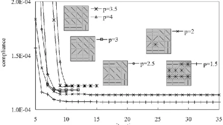
Figure 5: Influence of the penalization factor p of the BCP scheme upon the optimization results The influence of the penalization factor p on the optimization results is investigated in Fig. 5. For different values of p, the optimization iterations are quite stable, but the compliances and orientation layouts are different in the optimization results. As in topology optimization, a smaller penalization factor leads to stiffer design optimums. However, a too small penalization factor ‘p’ makes the optimization iteration converge quite slowly. In the cases of
p=2 and p=1.5, the optimization processes have not converged after 30 iterations, while the other tests need about
10 to 15 iterations. Besides, there are still some patches consisting of “mixed” material for these two tests after even 50 iterations, as shown in Fig. 5. As a conclusion, the suggested value for the penalization factor isp
2.5, 4
.6.2. Natural frequency maximization
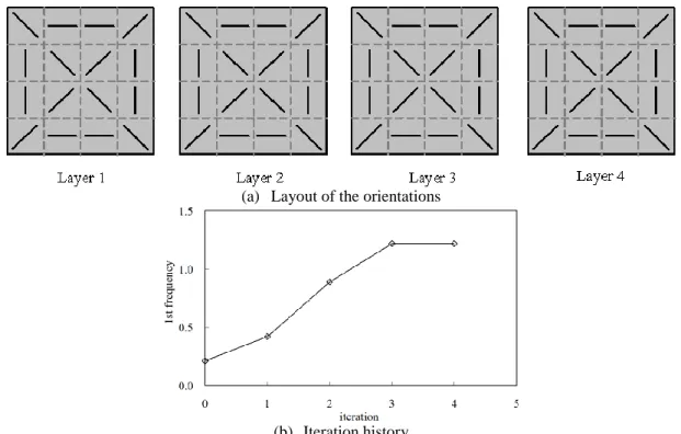
We consider a 4-layer square plate whose four corners are simply fixed (see Figure 6). The plate size is 4×4m and the total thickness is 0.1m. Each layer is meshed into 16×16 quadrangular solid shell elements and 4×4 patches. As a result, there are totally 64 designable patches.
Figure 6: Model of a 4-layer square laminate
Assume Material 1 (see Table 4) is adopted and four candidate orientations (90/45/0/-45) are used. First, the fundamental frequency is maximized without volume constraint. The optimal layout is obtained very quickly after 4 iterations. As shown in Fig.7, all layers have the same layout. Here, layer 1 refers to the bottom layer and layer 4 the top one.
Now, the volume constraint related to eq. (18) is added into the optimization model and suppose only 75% patches can be filled with material 1. As shown in Fig. 8(a), both bottom and top layers are exactly the same as those without volume constraint in Fig.7. For the middle layers, 8 patches near the edges are void while the filled patches have the same fiber orientations as those in Fig.7. The optimization iteration curves are plotted in Fig. 8(b).
(a) Layout of the orientations
(b) Iteration history
Figure7: Optimization results of the fundamental frequency maximization
(a) Layout of the orientations
(b) Iteration history
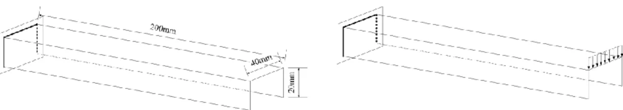
Figure 8: Optimization results of the fundamental frequency maximization with volume constraint 6.3. Four-layer laminated U-beam
The beam is shown in Figure 9a. The thickness of the laminate is 1mm. Quadrangular multi-layer solid shell elements in Samcef are used to discretize the laminate beam with a basic mesh size of 4×4mm2 and all elements can be designed independently. The element stiffness matrix related to each layer of each candidate orientation is extracted for sensitivity analysis. The beam is clamped at one end and a uniform line force is applied on the other end, as shown in Figure 9b. Suppose both flanges have a symmetrical fiber orientation layout and only one flange is shown for all optimization results.
Figure 9: Model of a 4-layer laminated beam. a/ geometry. b/ load case Table 5 Material properties (MC2)
glass-epoxy
Ex Ey Gxy vxy
54GPa 18GPa 9GPa 0.25
polymer-foam
E v
0.125GPa 0.3
Suppose now both orthotropic glass-epoxy with 4 candidate orientations and isotropic polymer-foam are available (see Table 5). The volume fraction of glass-epoxy is assumed to be less than 80% of the whole structure. According to eq. (18), the starting point is feasible for the penalization factor pV=1. As shown in Fig. 11(a), the
optimization process is stable and converges after 31 iterations. The optimal orientation layout is presented in Fig. 11(b). Layer 1 refers to the inner layer and layer 4 indicates the outer one. It is seen that the volume constraint is less than its upper bound at the starting point and stably increases to the upper bound. Meanwhile, glass-epoxy is placed at the loaded end of the beam, especially the vertical rib, while the polymer-foam, denoted by gray, occupies the fixed end and inner layer. Meanwhile, glass-epoxy of orientation 0/-45 degree is not used in the final layout.
7. Conclusions
In this paper, we present a novel parameterization scheme based on a bi-value coding for solving the discrete material optimization of composite structures. With a reduced number of design variables, the BCP scheme [6] generalizes the SFP scheme [2] and is a challenger to the classic DMO [11] for large-scale problems. Furthermore, the BCP formulation provides a well-posed problem for an efficient solution using sequential convex programming algorithms. Different penalization functions of intermediate densities have been proposed and the choice of the penalization parameters has been discussed. The on-going work is devoted to extend the application of this novel parameterization scheme to larger problems involving industrial composite structures including compliance, displacement, stress constraints but also buckling and perimeter constraints.
8. Acknowledgements
This work was supported by the Walloon Region of Belgium and SKYWIN (Aerospace Cluster of Wallonia), through the project VIRTUALCOMP.
Layer 4
Layer 3
Layer 2
Layer 1
Figure12 Optimization result of the 4-layer laminated beam under line force with volume constraint – Orientation layout
9. References
[1] M.P. Bendsøe, M. P. Optimal shape design as a material distribution problem. Structural Optimization, 1 (4), 193-202, 1989
[2] M. Bruyneel. SFP – a new parameterization based on shape functions for optimal material selection: application to conventional composite plies. Structural and Multidisciplinary Optimization. 43 (1), 17-27, 2011.
[3] M. Bruyneel and P. Duysinx. Note on topology optimization of continuum structure including self-weight.
Structural and Multidisciplinary Optimization. 29 (4), 245-256, 2005.
[4] M. Bruyneel, P. Duysinx, and C. Fleury. A family of MMA approximations for structural optimization.
Structural and Multidisciplinary Optimization, 24 (4), 263-276, 2002.
[5] M. Bruyneel, P. Duysinx, C. Fleury and T. Gao. Extension of the Shape Functions with Penalization for Composite-Ply Orientation. AIAA Journal, 49 (10), 2325-2329, 2011.
[6] T. Gao, W. Zhang, and P. Duysinx. A bi-value coding parameterization scheme for the discrete optimal orientation design of the composite laminate. Int. J. for Num. Methods in Engng. 91 (1), 98-114, 2012 [7] J.C. Halpin and S.W. Tsai. Effect of environmental factors on composite materials. AFML-TR, 67-423, June
1969.
[8] E. Lund, and J. Stegmann. On structural optimization of composite shell structures using a discrete constitutive parametrization. Wind Energy, 8, 109-124, 2005
[9] O. Sigmund and S. Torquato. Design of materials with extreme thermal expansion using a three-phase topology optimization method. Journal of the Mechanics and Physics of Solids, 45 (6), 1037-1067, 2000 [10] J. Stegmann and E. Lund. Discrete material optimization of general composite shell structures. Int. J. for
Num. Methods in Engng. 62 (14), 2009-2027, 2005
[11] M. Stolpe and K. Svanberg. An alternative interpolation scheme for minimum compliance topology optimization. Structural and Multidisciplinary Optimization, 22 (2), 116-124, 2001.
[12] J. Thomsen. Topology optimization of structures composed of one or two materials, Structural Optimization, 5(1-2): 108-115, 1992.
[13] J. Zhu, W. Zhang and P. Beckers. Integrated layout design of multicomponent systems. Int. J. for Num.