Optimal power dispatching strategies in smart-microgrids with storage

O

pen

A

rchive

T

OULOUSE

A

rchive

O

uverte (

OATAO

)

OATAO is an open access repository that collects the work of Toulouse researchers and

makes it freely available over the web where possible.

This is an author-deposited version published in :

http://oatao.univ-toulouse.fr/

Eprints ID : 11997

To link to this article : doi:10.1016/j.rser.2014.07.138

URL : http://dx.doi.org/10.1016/j.rser.2014.07.138

To cite this version : Rigo-Mariani, Rémy and Sareni, Bruno and

Roboam, Xavier and Turpin, Christophe Optimal power dispatching

strategies in smart-microgrids with storage. (2014) Renewable and

Sustainable Energy Reviews, vol. 40 . pp. 649-658. ISSN

1364-0321

Any correspondance concerning this service should be sent to the repository

administrator:

staff-oatao@listes-diff.inp-toulouse.fr

Optimal power dispatching strategies in smart-microgrids with storage

Rémy Rigo-Mariani

n

, Bruno Sareni, Xavier Roboam, Christophe Turpin

LAPLACE, UMR CNRS-INPT-UPS, ENSEEIHT, 2 Rue Camichel, 31 071 Toulouse, France

Keywords: Smart-grids

Optimal power dispatching Trust region algorithm Genetic algorithms Particle swarm Dynamic programming

a b s t r a c t

With the development of decentralized power sources based on renewable energy, power grids need smarter operations to be run properly. This paper investigates different procedures for the optimal power dispatching of a grid-connected prosumer with an energy storage consisting in a high speed flywheel. An off-line optimal scheduling for the day ahead aims at minimizing the cost with regards to the daily energy rates and considering the forecasts for both consumption and production. That dispatching is performed thanks to global optimization procedures based on a trust-region method or on a niching genetic algorithm. Another approach using step by step optimization and exploiting an original self-adaptive dynamic programming strategy is also developed. The paper discusses the performance of all the considered methods with regards to the obtained results and the computational time.

Contents

1. Introduction . . . 649

2. Power flow model of the microgrid . . . 650

2.1. Considered microgrid and constraints . . . 650

2.2. Equations and degrees of freedom . . . 651

2.3. Storage efficiency. . . 651

2.4. Input variables . . . 652

3. Optimal power dispatching problem . . . 652

4. Approaches for solving the optimal dispatching problem . . . 653

4.1. Global optimization of power flows . . . 653

4.2. Global optimization with a sampled problem . . . 653

4.2.1. Graph representation and Bellman–Ford algorithm. . . 653

4.2.2. Undetermined SOC levels . . . 654

4.2.3. Transition optimization . . . 654

4.2.4. Self-adaptive DP. . . 655

5. Simulations and results . . . 656

5.1. Performance and computational time of the power dispatching procedures . . . 656

5.2. Storage benefits . . . 656

6. Conclusions . . . 657

Acknowledgment . . . 657

References . . . 657

1. Introduction

Global energy consumption has increased by 50% since the 90's and is expected to keep going up with a ratio of 1.6% per year due to the growing population on earth and the new needs that have

http://dx.doi.org/10.1016/j.rser.2014.07.138 n

Corresponding author: Tel.: þ33 5 34 32 23 56.

emerged[1]. To face that increasing demand of electrical power in compliance with the liberalization of the electricity market and the need of reducing CO2 emissions, many distributed energy resources have appeared and especially the generation systems that utilize renewable energy sources. Thus, distribution networks evolve towards more meshed structures, and they are likely to become associations of a large number of “microgrids” combining both consumption and production and interacting with the main grid [2]. Due to the stochastic nature of those generations, it requires smarter operations to keep feeding loads in a supply-on-demand system. The improvements in storage technologies allow those operations with a more flexible and reliable management of energy [3]. Renewable energy sources associated with storage units are then considered like active distributed generators, one of the fundamental elements of the “Smart Grid” concept[4]. Adding a storage device deeply questions the most widely used model that consists in selling all the highly subsidized production at important prices and buying the whole consumption. It also allows the owners of microgrids to optimize the power exchanged with the main grid in compliance with the electricity market and the forecasts for the day ahead [5]. Thus, more and more methods based on optimization algorithms are developed to perform the optimal scheduling of power flows within the hybrid electrical systems with load, production and storage[6,7]. In the microgrid considered in this study, all the components are connected through a DC bus (Fig. 1a) with the following data:

!

Consumption: A building with a maximum contractual power of 156 kW.

!

Production: Solar PV arrays with a total capacity of 175 kWp.

!

Storage: A 100 kW/100 kWh storage consisting in ten 10 kW/ 10 kWh high speed flywheels.

In this paper, an off-line optimal power dispatching problem is introduced with the aim of minimizing global energy cost, con-sidering the forecasts for consumption and production and the possible constraints imposed by the main grid operator. The second section describes the power flow model used to represent the system and the corresponding equations. Then, the next part refers to the proposed optimization methods using an evolution-ary algorithms or a trust region strategy that both consider the global load consumption and the PV production over the day. A step by step optimization based on basic Dynamic Programming

(DP) is also presented and an original self-adaptive DP is devel-oped. Finally, some results performed with the various algorithms are exposed and discussed, especially in terms of reliability, efficiency and computational time.

2. Power flow model of the microgrid

2.1. Considered microgrid and constraints

Voltages and currents are not considered so far. The study refers to the optimization of active power flows piwhich appear to

be a widely used formulation for such a problem[8,9]. A nomen-clature of all the used symbols is given inTable 1. Eleven power flows are identified to entirely characterize the system at each time step.

!

p1: power flowing through the consumption meter

!

p2: power flowing between the DC bus and the consumption branch after the converter

!

p3: power flowing between the DC bus and the consumption branch before the converter

!

p4: power flowing between the storage and the DC bus after the converter

!

p5: power flowing between the storage and the DC bus before the converter

!

p6: power flowing between the production branch and the rest of the DC bus

!

p7: effective solar production after the converter

!

p8: effective solar production before the converter

!

p9: derating of the solar production in case of microgrid congestion (section 2.2)

!

p10: power flowing through the production meter before the converter

!

p11: effective production sold

Due to the grid policy, three system constraints have to be fulfilled at each time step t:

!

Pp(t)Z0: the power cannot return to the grid through the

consumption meter.

!

Ps(t)Z0: the main grid cannot feed the DC bus through the

production meter.

!

Pprod_c(t)Z0: the storage cannot be discharged through the

production meter.

A particular attention is attached to the grid power Pgrid(t)

which should comply with requirements possibly set by the grid operator Pgrid_minand Pgrid_max:

PgridðtÞ ¼ PpðtÞ % PsðtÞ ð1Þ

Pgrid_minðtÞ o PgridðtÞ o Pgrid_maxðtÞ ð2Þ

2.2. Equations and degrees of freedom

Equations are generated using the graph theory and an inci-dence list to describe the system with particular equations corresponding to each type of node [10]. In Fig. 1b, the black arrows between nodes represent sign conventions for power flows while the possible directions (mono or bi-directional) are illu-strated by the dotted arrows. Three degrees of freedom are required to control the whole system (Fig. 1a):

!

Pst(t): the power flowing from/to the storage unit

!

Pprod_c(t): the power flowing from the solar PV arrays to the

common DC bus

! Δ

PPV(t): denotes the possibility to decrease the solar PV

production (MPPT derating) in order to fulfill grid constraints, in particular when the power supplier does not allow (or limits) injection of the solar PV production to the main grid (Pgrid_min).

For instance, if the flywheels are fully charged while production is greater than consumed energy and if no injection is allowed

to the grid, a part of the produced energy should be wasted to fulfill the main grid constraints.

Those degrees of freedom being set from a management process, all power flows in the microgrid can be expressed from the consumption Pload(t) and production Pprod(t) and from the

input data, i.e.

η

CVS,i(typically

η

CVS,i¼95%) the efficiency related to

the power converter corresponding to the node i. From the graph representation, subsequent equations can be derived:

p1ðtÞ ¼ PloadðtÞ % p2ðtÞ ð3Þ p2ðtÞ ¼ p3ðtÞ þ 1% 1 η_CVS;3 ! : maxð0; % p3ðtÞÞ þ ðηCV S;3%1Þ: maxð0; p3ðtÞÞ ð4Þ p3ðtÞ ¼ p4ðtÞ þ p6ðtÞ ð5Þ p₄ðtÞ ¼ p₅ðtÞ þ 1 % 1 ηCVS;5 ! : maxð0; %p₅ðtÞÞ þ ðηCV S;5%1Þ: maxð0; p5ðtÞÞ ð6Þ p7ðtÞ ¼

η

CVS;8:p8ðtÞ ð7Þ p₈ðtÞ ¼ PprodðtÞ % p9ðtÞ ð8Þ p10ðtÞ ¼ p7ðtÞ % p6ðtÞ ð9Þ p₁₁ðtÞ ¼

η

CV S;11:p10ðtÞ ð10Þ

Note that in(4) and (6)the power flows through converters are bidirectional. Two cases are identified depending on the direction of the flows to determine how the corresponding converter efficiency

η

CVS,ihas to be considered. That is performed using the

max function:

maxða; bÞ ¼ a if a Zb maxða; bÞ ¼ b if a ob (

ð11Þ The next sections only refer to the flows Pp, Ps, Pgridand the

degrees of freedom that are the truly interesting powers in term of management.

2.3. Storage efficiency

The storage losses are computed versus the state of charge SOC (in %) and the power Pstusing a function Ploss(SOC) and calculating

the efficiency with a fourth degree polynomial interpolation

η

FS(Pst) as shown in(11). Interpolations are extracted from

experi-mental measurements provided by the manufacturer. Note that due to confidentiality constraints, no additional information related to quantitative data have been allowed to be provided. Both Plossand

η

FSfunctions are also extracted from measurements

provided by the manufacturer. Another coefficient KFS(in kW) is

also introduced to estimate the self-discharge of the flywheels when they are not used [11]. Once the overall efficiency is computed, the true power PFS associated with the flywheel is

calculated as well as the SOC evolution using the maximum stored energy EFS(here 100 kWh), the time step

Δ

t(typically 1 h for the

off-line optimization) and the control reference p5.

PstðtÞ o0-PFSðtÞ ¼ PstðtÞ &

η

FSð % PstðtÞÞ PstðtÞ 40-PFSðtÞ ¼ PstðtÞ=

η

FSðPstðtÞÞ

(

ð12Þ Thus, when a power p5is required from the storage (i.e. p540), the actual power PFSincluding the flywheels losses is computed to

estimate the loss of stored energy that have to be decreased to the discharge power. The same process is performed when p5becomes negative for storage charging. If no power flows from/to the flywheels, the loss of stored energy is limited to the

self-Table 1

Nomenclature of the used symbols.

Pload Consumed power kW

Pprod solar PV production kW

pi power flows used to characterize the system (Section

2.1)

kW

Pp power flowing through the consumption meter kW

Ps power flowing through the production meter kW

Pst power flowing from/to the storage unit kW

PFS power flowing from/to the flywheel taking account of

device losses

kW Pst_min,

Pst_max

lower and upper bounds for Pst kW

EFS maximum stored energy in the storage unit kWh

KFS self-discharge coefficient of the flywheels (Section 2.3) kWh/

h ηFS flywheels efficiency depending on the exchanged power

Pst

–

SOC state of charge of the storage unit %

SOCmin,

SOCmax

lower and upper bounds for the SOC level % SOCstart,

SOCend

initial and final daily values for the SOC level % Pgrid power flowing between the main grid and the microgrid kW

Pgrid_min,

Pgrid_min

lower and upper bounds for Pgridpossibly set by the

power supplier

kW ηCVS,i efficiency of the ith converter in the graph

representation (Fig. 1b)

-ΔP%

PV solar production derated in case of microgrid congestion

(Section 2.2)

kW Cpurchase instantaneous cost for the purchased energy €/kWh

Csale instantaneous cost for the sold energy €/kWh

t time step h

Pref matrix with the scheduled controls for the degrees of freedom

kW C(Pref) daily cost to be minimized by the optimization

algorithm

€

Cnl vector with the non linear constraints of the optimization problem

discharge coefficient:

PstðtÞ a0-SOCðt þ

Δ

tÞ ¼ SOCðtÞ %PFSðtÞ&EFSΔt&100

PstðtÞ ¼0-SOCðt þ

Δ

tÞ ¼ SOCðtÞ %KFS_E&Δt

FS &100 8

<

:

ð13Þ The energy management strategy must ensure that both power and energy bounds are fulfilled with regards to storage power limits, i.e. Pst_min¼ %100 kW and Pst_max¼100 kW. With a storage

assumed to be charged at SOCstart¼50% at the beginning of the

day, the solving procedures should fulfill both upper and lower energy limits (i.e. SOCmin¼0% and SOCmax¼100%) while ensuring a

final value SOCend¼50%.

2.4. Input variables

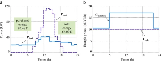
The energy management strategy is based on consumption and production forecasts similar to the example depicted inFig. 2a. The consumption profile is computed using measurements performed on the microgrid site and the production forecast uses a geophy-sical model considering among other the incidence and orienta-tion of the solar PV arrays[12,13]as well some estimation of the radiated energy on the microgrid site for the corresponding day.

The energy prices result from one of the fares proposed by the French main energy supplier. The purchase cost Cpurchasehas night

and daily values with 0.10 €/kWh from 10 p.m. to 6 a.m. and 0.17 €_{/kWh for the other time steps. An average fare of Csale¼0.10 €/kWh} is also considered for the production meter (Fig. 2b). Finally, an additional grid power constraints is introduced with P grid_-max¼0 kW between 7 p.m. and 10 p.m. with the aim of imposing

the microgrid autonomous operation during this period. Otherwise the bounds are set to high values (typically 103 _{kW). Without} storage device and optimal management, all the consumption is purchased from the grid while the PV production is sold. The resulting cost for that initial situation (noted Init) is 28.39 €. If the self-consumption of the production is considered, the generated energy feds the loads and the surplus is sold. In that case (noted SelfCons) the overall cost is of 5.82 €. Note that in both situations the previous grid constraints cannot be fulfilled by the microgrid. 3. Optimal power dispatching problem

The problem consists in planning, for each hour of a 24h-period, the best power dispatching that ensures the minimal energy cost of the microgrid while complying with the grid requirements. The decision variables computed in a vector Pref are the degrees of freedom defined in the previous section

according to upper and lower bounds respectively computed in vectors uband lb.. Those bounds can be expressed using a vector J24composed of 24 values equal to one. With a time step of 1 h, the total number of decision variables is 72.

Pref¼ ½P5ðtÞ P6ðtÞ P9ðtÞ(with t A½0::24 h(; noted P ¼ ½P5 P6

Δ

P9(

lb¼ ½Pst_min:J24 0:J24 0:J24(

ub¼ ½Pst_max:J24

η

CV S;8:PprodPprod( ð14Þ

The overall cost to be optimized is the difference between the sold and purchased energies during the day obtained by calculating the flows Ppand Psall along the simulated period (typically 24 h) for a

set of parameters Pref:

CðPrefÞ ¼ ∑ 24 t ¼0

CpurchaseðtÞ U PpðtÞ % CsaleUPsðtÞwith

Δ

t ¼1 h ð15Þ

Some constraints in the microgrid are implicitly included in the bounds previously defined. Additional constraints are added in order to fulfill all power flow requirements defined inSection 2. Eq.(16)allows controlling the powers though the meters that have both to remain positive with the given convention and set the two corresponding constraints CPpand CPs.

CPp¼ ∑ 24h t ¼0 max ð0; %PpðtÞÞ2 CPs¼ ∑ 24h t ¼0 max ð0; %PsðtÞÞ2 8 > > > > < > > > > : ð16Þ

The possible bounds set by the grid operator for Pgrid are

considered by summing all the overshoots. The negative and positive deviations are computed in constraints CPgrid% and CPgridþ .

CPþ grid¼ ∑

24h t ¼0

max ð0; PgridðtÞ % Pgrid_maxðtÞÞ2 CP%

grid¼ ∑ 24h t ¼0

max ð0; Pgrid_minðtÞ % PgridðtÞÞ2

8 > > > > < > > > > : ð17Þ

The three last limits refer to the use of the storage unit. Indeed the SOC has to remain between its lower and upper bounds and return at a given value at the end of the day (i.e. t¼24 h). The corresponding constraints are noted CSOC%

, CSOCþ

and CSOCend.

CSOCend¼ SOCð24hÞ %SOCend CSOCþ_¼24h_∑

t ¼0

max ð0; SOCðtÞ%SOCmaxÞ2 CSOC%_¼

∑ 24h t ¼0

max ð0; SOCmin% SOCðtÞÞ2

8 > > > > > > < > > > > > > : ð18Þ

0

6

12

18

24

0

40

80

120

0

6

12

18

24

0

5

10

15

20

Temps (h)

Temps (h)

P

o

w

er

(k

W

)

E

n

erg

ie

p

ri

ce

s

(c

€

/k

W

h

)

P

prod

P

load

_C

sale

C

purchase

purchased

energy

95.48 €

sold

energy

66.09 €

All those constraints are strongly nonlinear due to the bi-directional characteristic of static converters and the flywheel efficiency. They are computed in a vector Cnlthat will be used in the algorithms developed to optimize the energy management. Cnl¼ ½CPp CSOC% CSOCþ CSOCend CPgridþ CPgrid% ( ð19Þ

For all the constraints (except CSOCend), the returned value is

computed as the sum of the instantaneous violations determined with the max function all along the day. For instance, considering

(16), if Ps(t) is negative, the instantaneous violation is expressed as

the square value of the power flow. Then, the overall correspond-ing constraint for the dispatchcorrespond-ing problem is the sum of all overshoots. The final optimal dispatching problem consisting in managing the power flows for the day ahead with 1 h of time step could be considered as a long term scheduling. In real time, a short term scheduling (with a shorter sampling period) has to be run to take account of the differences between the actual values and the forecasts for the production and consumption [14]. At a lower level, an efficient control loop has to be implemented to manage the current/voltage references for the different converters accord-ing to the values returned by the short term schedulaccord-ing. Those two last problems are not the aim of the paper but are crucial in the field of smart microgrids[15].

4. Approaches for solving the optimal dispatching problem

4.1. Global optimization of power flows

The optimal dispatching in microgrids could be solved using step by step decisions with rules based methods such as state machine or fuzzy logic[16,17]. A great part of studies referring to scheduling in such systems use algorithms that consider the whole profiles and perform the global optimization of the mission for the entire time horizon (here 24 h). For instance, linear programming is often performed to control of the system on a large time scale

[9,18]. In this paper, three procedures are firstly investigated to manage optimal scheduling considering the mission all along the day.

The first optimization approach is a trust-region-reflective algorithm [19]. That method aims at solving the problem by approximating the objective function with a simpler quadratic function in a trust-region area. From an initial starting solution, the algorithm minimizes the cost while fulfilling all constraints and returns the best solution Pref

n

within the predefined bounds: Pn ref¼ ½P n st P n prod_c

Δ

P n PV( ¼arg min Pref ðCðPrefÞÞwith Cnlr0 ð20Þ The second method uses the clearing algorithm [20] a niching genetic algorithm which preserves diversity in the population in order to avoid premature convergence. The particle swarm

optimization method [21] is lastly used to solve the power management scheduling [22]. For those metaheuristics, all con-straints related to power flows are included in the cost function with a classical exterior penalty approach. The algorithm returns the best individual in the population (or in the particle swarm) from a given number of iterations:

Pn ref¼ ½P n st P n prod_c

Δ

P n PV( ¼arg min Pn ref CðPrefÞ þ

λ

:∑ i CnlðiÞ ! ð21Þ where the penalty coefficient

λ

is set to 106 _{to ensure the} constraints fulfilment.

4.2. Global optimization with a sampled problem 4.2.1. Graph representation and Bellman–Ford algorithm

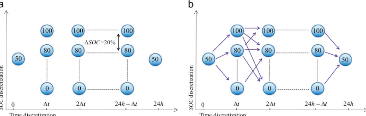
Just like the three methods previously exposed, the approach presented in this section optimizes the whole mission (i.e. the references for the degrees of freedom for the whole day). The problem is here represented as a succession of possible discrete states characterized by a time position t over one day and a state of charge

SOC[23]as shown inFig. 3a. With both SOCstartand SOCendfixed in the

problem there is only one available state for the initial and final time step. The mix of individual states taken for each time step returns a

SOCprofile all along the day that corresponds to a given solution Pref computed with all the instantaneous controls ensuring transitions between the selected states. Finding the best solution Pref

n

is equivalent to estimating the shortest path in terms of cost from the initial state to the final one. That is the base of the Dynamic Programming (DP) approach as developed here.

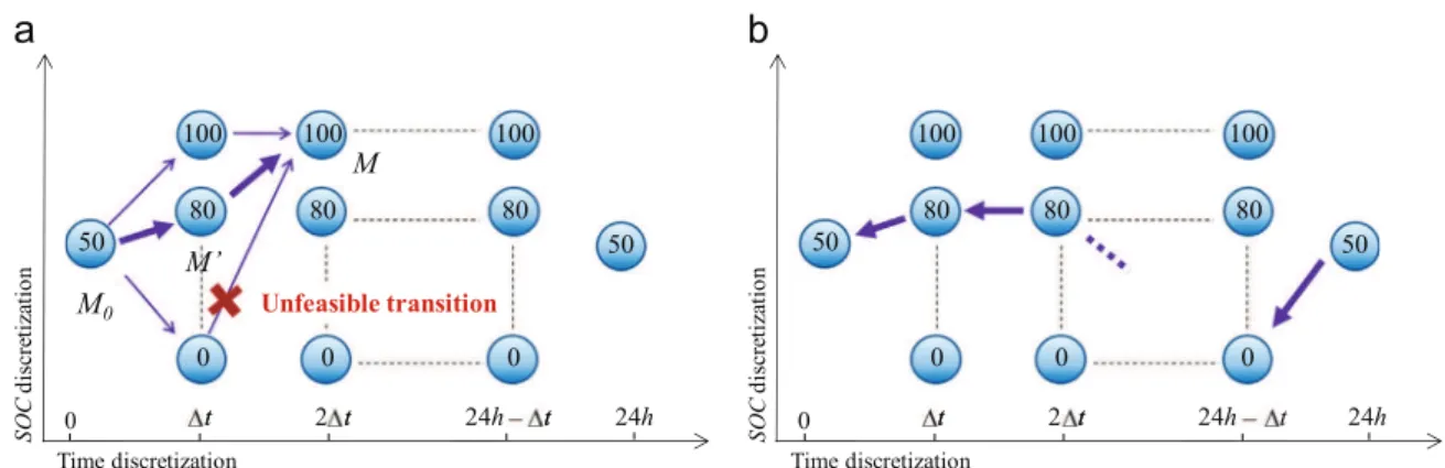
The cost of a solution equals to the sum of all the individual costs referring to the transitions between states. Thus, the Dynamic Programming requires computing all the transitions between the states situated at two successive time step (Fig. 3b). Transition are studied with regard to the instantaneous cost that depends on the values of the consumption and production as well as the instantaneous references of the degrees of freedom. The estimated cost of a transition is optimized as explained inSection 4.2.3. This cost is highly penalized if the corresponding transition appears to be infeasible due to the non-fulfilment of the system constraints (e.g. non fulfilment of the bounds associated with the main grid power Pgrid).

Once all transitions are studied, it is possible to determine the shortest path (i.e. the lowest cost) that allows reaching a state M starting from the initial point M0. At the previous time step, the obtained shortest path goes through the “predecessor” of M and denoted as M' (Fig. 4a). The predecessors of all the states are then determined moving forward for successive time steps. When all the predecessors are known, the optimal path is rebuilt backward from the final state using the Bellman–Ford algorithm [24]

(Fig. 4b). The returned solution Pref n

is the concatenation of all

the instantaneous controls of the power flows which relate to the degrees of freedom that allow to follow the optimal path.

4.2.2. Undetermined SOC levels

Moving from one SOC level to another consists in finding the best instantaneous degrees of freedom Pst(t), Pprod_c(t) and

Δ

PPV(t)

that ensure the transition with the lowest cost. Note that a transition between two pre-determined states of charge implicitly imposes the power value flowing through the storage unit Pst(t). However, in some cases, this can lead to the non-fulfilment of the grid constraints and the impossibility to ensure the transition. The resulting cost would be would be penalized.Fig. 5illustrates a case with fictive values without considering losses. In this example, there is no production and the grid operator imposes a consump-tion to a given value Pgrid(t) different from Pload(t). Thus Pprod_c(t)¼

Δ

PPV(t)¼0 and then Pst(t) should fed the difference Pgrid(t)%

Pload(t). That value does not necessary comply with the transition

between two predetermined states of charge and a non conver-gence of the algorithm could occur.

The previous algorithm is then modified with the aim of relieving the storage constraints by considering a space search 7

δ

around a predetermined SOC. The initial value of

δ

is set to

Δ

SOC/2 and is progressively reduced in case of non-convergence (typically

δ

’

δ

/2). In the example given inFig. 5, moving towards undetermined SOC levels allows ensuring the transition starting from a SOC equal to 40% and could avoid a non convergence of the overall Dynamic Programming algorithm.

4.2.3. Transition optimization

As already said, studying a transition between two states M and

M' consists in minimizing the cost while adapting the state of

charge for the next time step. This is performed using the trust region algorithm with a simpler problem than in the case with the global dispatching in so far as the number of decision variables simply equals here the number of degrees of freedom (i.e., three in the studied case). The bounds associated with the degrees of freedom as well as the grid constraints are expressed using the instantaneous values of the consumption and production. The storage constraints defined in(18)are modified in order to comply with the studied transition and adapt the SOC at the following state with SOC'7

δ

:

CSOCþ_{ðtÞ ¼maxð0; SOCðt þ}

Δ

tÞ % SOC0_þ

_δ

_Þ CSOC%_{ðtÞ ¼maxð0; %SOC}0_%

_δ

_{% SOCðt þ}

Δ

tÞÞ ð22Þ

Finally, the local optimal dispatching problem to be solved at each time step can be expressed as:

PrefðtÞ ¼ ½PstðtÞ Pprod_cðtÞ

Δ

PPVðtÞ(

lb ¼ ½Pst_min 0 0(

ub ¼ ½Pst_max

η

CVS;8:PprodðtÞ PprodðtÞ(

Pn refðtÞ ¼ ½P n stðtÞP n prod_cðtÞ

Δ

P n PVðtÞ( ¼argmin PrefðtÞ ðCpurchaseðtÞ:PaðtÞ % CsaleðtÞ:PsðtÞÞ with Ct

nlðPrefðtÞÞ ¼ ½CPaðtÞ CPsðtÞ CSOCþðtÞ CSOC%ðtÞ

&CPgrid% ðtÞ CPgridþ ðtÞ( r0 ð23Þ

Fig. 4.Dynamic Programming – (a) Computation of the predecessors and (b) optimal path rebuilt.

4.2.4. Self-adaptive DP

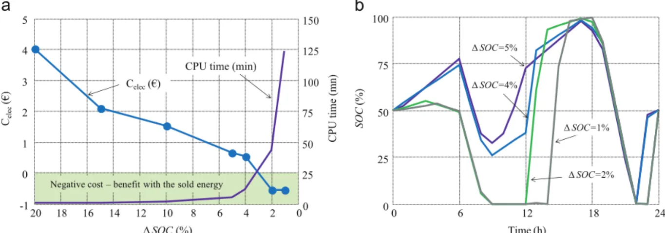
The DP returns good solutions but some preliminary results shows that its efficiency and convergence strongly depends on

Δ

SOCand

δ

. As shown inFig. 6a, the cost is improved with the

reduction of

Δ

SOC while the computational time required to obtain the optimal solution is drastically increased. Note that the trajectories obtained for different values of

Δ

SOCshows the same energy balance of the storage which is discharged at the beginning

Δ SOC=4% 0 2 4 6 8 10 12 14 16 18 20 -1 0 1 2 3 4 5 0 25 50 75 100 125 150 0 6 12 18 24 0 25 50 75 100 Celec(€)

CPU time (min)

Celec (€ ) CPU time (mn) Δ SOC (%) SOC (%) Time (h) Δ SOC=1% Δ SOC=2% Δ SOC=5%

Negative cost – benefit with the sold energy

Fig. 6.DP results for different SOC level of accuracy: (a) Cost and CPU time – (b) Storage energy.

ΔSOC1

ΔSOC2

ΔSOC1

Step 1:

Corse DP run with a

large ΔSOC sampling value

Step 2:

Space search and

number of states reduction

Step 3:

New DP run with a

smaller SOC sampling on the

reduced area (ΔSOC2=ΔSO

C

1

/2)

Fig. 7.Illustration of the self-adaptive Dynamic Programming.

Table 2

Performance of the trust-region reflective algorithm on the dispatching problem.

Pref01 Pref02 Pref03 Pref04

Starting point [PloadPprodPprod] [Pload0.J240.J24] [0.J240.J240.J24] [0.J24Pprod0.J24]

Convergence no yes no yes

C (Prefn) (in €) x 4.09 x 6.63

CPU time 33 s 24 s 1 s 16 s

Table 3

Performance of the clearing algorithm on the dispatching problem.

Number of generations 1000 5000 10,000 25,000 50,000

Cost – Average Values (€) 3.8071.08 1.6270.95 1.2570.81 0.9670.52 0.8770.38

Cost best values (€) 2.53 1.11 0.79 0.69 0.66

Average CPU Time (s) 6 min 35 min 1 h 10 min 2 h 45 min 5 h 30 min

Table 4

Performance of the particle swarm algorithm on the dispatching problem.

Number of Generations 1000 5000 10,000 25,000 50,000

Cost -Average Values (€) 23.63723.96 19.04 719.51 18.79719.89 17.86719.75 17.80719.81

Cost – best values (€) 9.35 6.48 4.99 4.90 4.90

of the day. Then the SOC increases when there is a great amount of solar production during the day. From 7 p.m. to 9 p.m., the flywheels are used to fulfill the grid constraints before returning to the desired state of charge at the end of the day. That optimal energetic behavior is found with great

Δ

SOC. Indeed, decreasing the discretization allows reducing the cost by optimizing the losses within the elements of the microgrid.

In order to get the best solution corresponding to the finest SOC sampling without a prohibitive CPU time, a self-adaptive DP (SDP) has been developed. At first, a basic DP is performed with a coarse

Δ

SOC. Then, a space search is defined around the obtained solution meaning that the number of possible states is reduced around the optimal profile. Afterwards, a new DP is computed considering the reduced search space with a smaller

Δ

SOC. As illustrated inFig. 7, the self-adaptive DP consists in a succession of basic DP optimizations starting with a large

Δ

SOC and decreasing it to smaller values. At each iteration, the search space is reduced by considering a new area around the optimal path. Then, this area is refined by discretizing it with a smaller value of

Δ

SOC(typically

Δ

SOC¼

Δ

SOC/2).

5. Simulations and results

5.1. Performance and computational time of the power dispatching procedures

In this section, the results obtained with the different proce-dures are compared with regard to the cost function value and the

computational time. All tests are performed by considering a time step of 1 h and with the production and consumption profiles defined inSection 2.Table 1shows the outputs of the trust region reflective algorithm with a maximum number of iterations equal to 150. Four starting points Pref0i are considered. They do not necessarily fulfill the constraints and correspond to various assumptions such as providing all the consumption though the storage for instance. The convergence only occurs in half of the cases and the obtained results depend on the starting points (Table 2).

Tables 3 and 4show the best results obtained by the nature inspired metaheuristics (i.e. clearing and PSO) after 10 indepen-dent runs. Average values with 95 % level of confidence as well as the best results are presented. Performances become greater with high numbers of generations with a population size equal to 100 elements in the two algorithms. Both strategies are more reliable than the trust-region method with better accuracy for the genetic algorithm but their CPU time up to 2 h is rather expensive.

The self-adaptive DP gives the best results with a good accuracy and a reduced computational time (Table 5). A solution with accuracy of

Δ

SOC ¼1% is finally reached after 10 min instead of 2 h with the basic DP. It should be noted that the small deviation on the cost between the basic DP with

Δ

SOC¼1% and the self-adaptive DP can be explained by different optimal paths found due to distinct values of

δ

around SOC levels during the search.

5.2. Storage benefits

Performance is now studied with regard to the optimal power profiles found with the solution returned by the SDP and noted PrefSPD.Fig. 8ashows that the grid power fulfils the constraints between 7 p.m. and 9 p.m. The storage is discharged at the beginning of the day in order o lower the cost when prices are higher (after 6 a.m.). Then the solar production feds the loads and charges the flywheels. At the end of the day the storage is fully used to satisfy the constraints before returned to the desired value

SOCend(Fig. 8b).

The optimal power sharing obtained with the SPD is illustrated inFig. 9 with few of energy purchased from the grid during the daily hours. The high amount of PV production is self-consumed in the loads and the storage. The surplus is even sold to the grid to get an additional benefit with a negative final electrical bill (Celec(PrefSDP) ¼ %0.17 €).

Table 5

Results obtained with the basic and self-adaptive DP.

ΔSOC 20% 15% 10% 5% 2% 1% SDP

Cost (€) 4.02 2.09 1.52 0.64 %0.56 %0.65 %0.17

CPU time 30 s 50 s 1 min 30 s 5 min 45 min 2 h 15 min 10 min

Table 6

Costs analysis for different cases.

Init SeflCon PrefSPD

Purchased energy (€) 95.48 39.18 23.43

Sold energy (€) 66.09 33.36 25.60

Constraint fulfillment no no yes

TOTAL (€) 28.39 5.82 %0.17

0

6

12

18

24

-100

-50

0

50

100

Grid constraints

fulfilled

PV production

self-consumed

Time (h)

P

gr id

(k

W

)

P

refSPD

0

6

12

18

24

0

25

50

75

100

Time (h)

S

O

C

(%

)

Init

The cost analysis of the solution PrefSDPis now compared with the electrical bills corresponding to the cases Init and SelfCon. The best cost corresponds to a case with storage and optimal management (Table 6). Less production is sold but the self-consumption allows reducing the bill by lowering the purchased energy when prices are higher. Note that with no storage the grid constraints cannot be fulfilled. This could lead to pay additional penalties to the grid operator. On the contrary encouraging the constraints fulfillment with additional benefit could allow justifying the implementation of a storage unit whose cost has not been considered so far in the study.

6. Conclusions

In this paper, various optimization approaches have been compared in order to perform the optimal dispatching of power flows in a grid connected smart system involving loads, decen-tralized sources of renewable energy (solar PV panels) and flywheels as storage unit. In particular, an original self-adaptive method based on DP has been developed to enhance the perfor-mance in terms of cost with rapid convergence. For the given hypothesis and constraints relative to grid consumption and solar PV production, this method was revealed more efficient than a classical trust-region based approach and a evolutionary algo-rithms. All investigated procedures take account of the forecasts of consumption and production and aim at generating the best power dispatching for the day ahead. In real-time, an additional control has to be performed so as to ensure the predicted efficiency by correcting the possible forecast errors as described in[14]. Further works will also investigate the generalization of the approach for more complex microgrid architectures including other parameters, e.g. multiple energy storages of different nature (flywheels, electrolyzer-fuel cell association, batteries), various energy rates related to the cost of the grid power depending on the target load (storage charge or consumer feeding) and other grid services such as peak shaving or grid disconnection. Finally, additional studies will focus on the coupling between the sizing of the storage and the energy management aiming at optimizing the tradeoff between the cost of the storage systems and the reduction of the microgrid energy consumption by considering simulations over a longer period of time.

Acknowledgment

This study has been carried out in the framework of the SMART ZAE national project. The authors thank the project leader

INEO-SCLE-SFE and partners LEVISYS and CIRTEM for their support and Colomiers high school for providing the data of solar irradiation. The SMART ZAE project is supported by ADEME (Agence de l'Environnement et de la Maîtrise de l'Energie)

References

[1] Conti J, Holtberg PD, Beamon JA, Napolitano SA, Schaal AM, Turnure JT. Annual energy outlook. US energy information administration; 2011. Available at: 〈http://www.eia.gov〉.

[2] Celli G, Pilo F, Pisano G, Allegranza V, Cicoria R, Iaria A. Meshed vs. radial MV distribution network in presence of large amount of DG. Power Systems Conference and Exposition IEEE PES; 2004.

[3] Yeleti S, Fu S. Impacts of energy storage on the future power system. North American Power Symposium (NAPS) 2010: 1–7.

[4] Lu D, François B. Strategic framework of an energy management of a microgrid with a photovoltaic-based active generator. ELECTROMOTION, EPE Chapter ‘_{Electric Drives' Joint Symposium; 2009, Lille, France.}

[5]Colson CM. A Review of Challenges to Real-Time Power Management of Microgrids. IEEE Power & Energy Society General Meeting 2009:1–8. [6]Banos R, Manzano-Agugliarob F, Montoyab FG, Gila C, Alcaydeb A, Gomezc J.

Optimization methods applied to renewable and sustainable energy: A review. Renewable and Sustainable Energy Reviews 2011;15:1753–66.

[7]Erdinc O, Uzunoglu M. Optimum design of hybrid renewable energy systems: Overview of different approaches. Renewable and Sustainable Energy Reviews 2012;16:1412–25.

[8]Nottrott A, Kleissl J, Washom B. Storage dispatch optimization for grid-connected combined photovoltaic-battery storage systems. Power and Energy Society General Meeting, IEEE 2012:1–7.

[9] Bagherian A, Moghaddas SM. A developed energy management system for a microgrid in the competitive electricity market. IEEE Bucharest Power Tech Conference; 2009.

[10]Harris JM, Hirst JL, Mossinghoff MJ. Combinatorics and Graph Theory. 2nd EditionSpringer; 2000.

[11]Hadjipaschalis I, Poullikkas A, Efthimiou V. Overview of current and future energy storage technologies for electric power applications. Renew Sustain Energy Rev 2009;13:1513–22.

[12]Darras C, Sailler S, Thibault C, Muselli M, Poggi P, Hoguet JC, et al. Sizing of photovoltaic system coupled with hydrogen/oxygen storage based on the ORIENTE model. Int J Hydrog Energy 2010;35:3322–32.

[13]Mehdaoui A, Sadok M, Chikhi SA, Mammeri A. Gain énergétique entre deux configurations de système de pompage d'eau photovoltaïque Application au site d'Adrar. Rev Energies Renouv 2010;13:571–82.

[14] Rigo-Mariani R, Sareni B, Roboam X, Astier S, Steinmetz JG, Cahuet E. Off-line and On-line power dispatching strategies for a grid connected commercial building with storage unit. In: IFAC Power Plant and Power System Control; 2012.

[15]Kanchev H, Lu D, Colas F, Lazarov V, François B. Energy management and operational planning of a microgrid with a PV-based active generator for smart grid applications. IEEE Trans Ind Electron 2011;58.

[16]Sechilariu M, Wang B, Locment F. Building integrated photovoltaic system with energy storage and smart grid communication. IEEE Trans Ind Electron 2013;60:1606–18.

[17]Manjili YS, Vega R, Jamshidi M. Cost-efficient environmentally-friendly control of micro-grids using intelligent decision-making for storage energy manage-ment. Intell Autom Soft Comput 2013;19:649–70.

Temps (h)

Temps (h)

0

6

12

18

24

0

40

80

120

0

6

12

18

24

0

20

40

60

P

con so

(k

W

)

P

pr od

(k

W

)

from the PV

from the grid

from the storage

to the loads

sold to the

grid

to the storage

[18]Bradbury K, Pratson L, Patiño-Echeverri D. Economic viability of energy storage systems based on price arbitrage potential in real-time U.S. electricity markets. Appl Energy 2014;114:512–9.

[19]Coleman TF, Li Y. An interior trust region approach for nonlinear minimization subject to bounds. SIAM J Optim 1996;6:418–45.

[20] Petrowski A. A clearing procedure as niching method for genetic algorithms. In: Proceedings of IEEE evolutionary computation; 1996: p. 798–803. [21] Kennedy J, Eberhart R. Particle swarm optimization. In: IEEE Proceedings of

the international conference on neural networks; 1995: p. 1942–8.

[22] Phuangpornpitak N, Tia S, Prommee W, Phuangpompitak W. A study of particle swarm technique for renewable energy power systems. In: International con-ference on energy and sustainable development: issues and strategies (ESD); 2010: p. 1–6.

[23] Riffoneau Y, Bacha S, Barruel F, Ploix S. Optimal power flow management for grid connected PV systems with batteries. IEEE Trans Sustain Energy 2011;2:309–19.

[24] Bertsekas P. Dynamic programming and optimal control. 2nd Edition, Athena Scientific; 2000.