Seasonal Time Series and Autocorrelation Function Estimation

Série Scientifique

Scientific Series

Montréal Octobre 1997

97s-35

Seasonal Time Series and Autocorrelation Function Estimation

Hahn Shik Lee, Eric Ghysels, William R. Bell

Ce document est publié dans l’intention de rendre accessibles les résultats préliminaires de la recherche effectuée au CIRANO, afin de susciter des échanges et des suggestions. Les idées et les opinions émises sont sous l’unique responsabilité des auteurs, et ne représentent pas nécessairement les positions du CIRANO ou de ses partenaires.

This paper presents preliminary research carried out at CIRANO and aims to encourage discussion and comment. The observations and viewpoints expressed are the sole responsibility of the authors. They do not necessarily represent positions of CIRANO or its partners. CIRANO

Le CIRANO est une corporation privée à but non lucratif constituée en vertu de la Loi des compagnies du Québec. Le financement de son infrastructure et de ses activités de recherche provient des cotisations de ses organisations-membres, d’une subvention d’infrastructure du ministère de l’Industrie, du Commerce, de la Science et de la Technologie, de même que des subventions et mandats obtenus par ses équipes de recherche. La Série Scientifique est la réalisation d’une des missions que s’est données le CIRANO, soit de développer l’analyse scientifique des organisations et des comportements stratégiques.

CIRANO is a private non-profit organization incorporated under the Québec Companies Act. Its infrastructure and research activities are funded through fees paid by member organizations, an infrastructure grant from the Ministère de l’Industrie, du Commerce, de la Science et de la Technologie, and grants and research mandates obtained by its research teams. The Scientific Series fulfils one of the missions of CIRANO: to develop the scientific analysis of organizations and strategic behaviour.

Les organisations-partenaires / The Partner Organizations

•École des Hautes Études Commerciales •École Polytechnique

•McGill University •Université de Montréal

•Université du Québec à Montréal •Université Laval

•MEQ •MICST •Avenor

•Banque Nationale du Canada •Bell Québec

•Caisse de dépôt et placement du Québec

•Fédération des caisses populaires Desjardins de Montréal et de l’Ouest-du-Québec •Hydro-Québec

•Raymond, Chabot, Martin, Paré •Scetauroute

•Société d’électrolyse et de chimie Alcan Ltée •Téléglobe Canada

•Ville de Montréal

Corresponding Author: Eric Ghysels, CIRANO, 2020 University Street, 25th floor, Montréal, Qc,

*

Canada H3A 2A5 Tel: (514) 985-4000 Fax: (514) 985-4039 e-mail: [email protected] The first author would like to acknowledge the support of the Bureau of the Census where part of the research was completed while he was a participant in the ASA/NSF/Census Research Program. The second author acknowledges the financial support of the Natural Sciences and Engineering Research Counsil of Canada and the Fonds FCAR du Québec.

Sogang University H

Pennsylvania State University and CIRANO I

U.S. Bureau of the Census

§

Seasonal Time Series and Autocorrelation

Function Estimation

Hahn Shik Lee , Eric Ghysels , William R. Bell

Résumé / Abstract

Lorsqu’on calcule une fonction d’autocorrélation, il est normal d’enlever d’une série la moyenne non conditionnelle. Cette pratique s’applique également dans le cas des séries saisonnières. Pourtant, il serait plus logique d’utiliser des moyennes saisonnières. Hasza (1980) et Bierens (1993) ont étudié l’effet de la moyenne sur l’estimation d’une fonction d’autocorrélation pour un processus avec racine unitaire. Nous examinons le cas de processus avec racines unitaires saisonnières. Nos résultats théoriques de distribution asymptotique, de même que nos simulations de petits échantillons, démontrent l’importance d’enlever les moyennes saisonnières quand on veut identifier proprement les processus saisonniers.

Time series are demeaned when sample autocorrelation functions are computed. By the same logic it would seem appealing to remove seasonal means from seasonal time series before computing sample autocorrelation functions. Yet, standard practice is only to remove the overall mean and ignore the possibility of seasonal mean shifts in the data. Whether or not time series are seasonally demeaned has very important consequences on the asymptotic behavior of autocorrelation functions (henceforth ACF). Hasza (1980) and Bierens (1993) studied the asymptotic properties of the sample ACF of non-seasonal integrated processes and showed how they depend on the demeaning of the data. In this paper we study the large sample behavior of the ACF when the data generating processes are seasonal with or without seasonal unit roots. The effect on the asymptotic distribution of seasonal mean shifts and their removal is investigated and the practical consequences of these theoretical developments are also discussed. We also examine the small sample behavior of ACF estimates through Monte Carlo simulations.

Mots Clés : Saisonalité stochastique et déterministe, identification de modèles, racines unitaires saisonnières, autocorrélation

Keywords : Deterministic/stochastic seasonality, model identification, seasonal unit roots, autocorrelation

1 Introduction

Since the work by Box and Jenkins (1976), it is standard practice to analyze the sample autocorrelation and partial autocorrelation functions in order to identify, specify and diagnose univariate models for seasonal time series, using the raw, first-differenced or seasonally-first-differenced data. Inspection of the characteristics of the autocorrelation function [henceforth ACF] was later complemented with formal statistical tests for unit-root nonstationarity. Since the work of Fuller (1976) and Dickey and Fuller (1979), testing for a zero-frequency unit root has become commonplace, and the properties of various testing procedures have been widely discussed. While testing for unit roots at the seasonal frequencies is a relatively more recent occurrence, it also has generated considerable interest with the tests proposed by Hasza and Fuller (1982), Dickey, Hasza and Fuller (1984), Hylleberg, Engle, Granger and Yoo (1990), Ghysels, Lee and Noh (1994), among others. The ACF is typically computed from demeaned data. Yet, seasonal means are almost never removed before computing the ACF in seasonal time series. It is perhaps somewhat surprising that the consequences of not removing seasonal mean shifts on the identification and specification of seasonal time series has hitherto received little attention. As for non-seasonal processes, Hasza (1980) and Bierens (1993) investigated the asymptotic properties of the sample ACF of integrated series, which depend on whether the data were demeaned. We study the large-sample behavior of the ACF when the data-generating processes are seasonal with or without seasonal unit roots. The effects of varying seasonal means are investigated, and the practical consequences of these theoretical developments are also discussed by examining the behavior of the ACFs before and after removing seasonal means. We show that there are some serious deficiencies in the usual model identification procedures which rely on simple demeaned data.

The paper is organized as follows. We first study the theoretical properties of the ACF for seasonal time series. Section 2 discusses the asymptotic distribution of the sample ACF for seasonal data which contain some roots on the unit circle and/or different means across different seasons. Section 3 reports the finite sample behavior of the ACF via Monte Carlo simulation. Section 4 reports some empirical results. Section 5 concludes with a brief discussion about the potential implications of the results for modeling seasonal time series.

2 Asymptotic Distribution of Sample ACF for Seasonal Processes

In applied time series analysis, an investigation of the sample autocorrelation structure often suggests the identification and specification of empirical models. In the well-known Box-Jenkins approach, this idea is often used in detecting certain types of nonstationarities in the data. In the first subsection, we discuss the limiting distribution of the sample autocorrelation function for a general nonstationary process with unit roots at seasonal frequencies as well as at the zero frequency. Our

ˆr_1k

2 k ' 2

2 k/ 2 ˆr_1k ' 'T_t'k%1(y_t&¯y)(y_t&k&¯y) / 'T_t'1(y_t&¯y)2

¯y ' 'T_t'1y_t/T.

y_t ' y_t&1 % u_t,

T(1& ˆr_1k) 6 k{ 2_k/ 2 % W(1)2 & 2W(1)I1₀W(r)dr % 2[I1₀W(r)dr]2} ÷ 2{I1₀W(r)2dr & [I1₀W(r)dr]2},

The sample autocorrelation coefficient has first index one, as it refers 1

to the Data Generating Process (henceforth DGP) appearing in (2.2), which corresponds to a first-difference stationary process. In general the first index will refer to the order of differencing.

Note that, when u is i.i.d., 2 _t and hence the expression in equation (2.3) reduces to 1.

analysis extends the results obtained by Hasza (1980) and Bierens (1993), who focused exclusively on the zero-frequency properties. The second subsection covers the case when seasonality in the data is caused by different seasonal means for different seasons.

2.1 Nonstationary series with some seasonal unit roots

It is well-known that the ACF of a stationary process decays towards zero, whereas that of a nonstationary process with a unit root at the zero frequency tends to stay near one. In particular, Hasza (1982) and Bierens (1993) have shown that the sample ACF for integrated processes converges in probability to one. It is shown in this paper that the behavior of the sample ACF is quite different from that of the usual integrated processes when unit roots at the seasonal frequencies are also present. To clarify this, suppose that we have T observations, (y ,y ,..., y ), of a time_{1 2 T} series process y . The sample ACF at lag k denoted r^ is then given by:_{t 1k}

(2.1)

where k $ 1 and 1 For an integrated process generated by

(2.2)

where u follows a martingale difference sequence obeying the conditions for the_t functional central limit theorem as, for instance, in Phillips (1987). It has been shown that the sample autocorrelation function converges in probability to one. Moreover, for any fixed integer k, Bierens (1993) shows that for r^ defined in_1k (2.1):2

2 k ' limT64T&1' T t'k%1E[(k&1/2' t j't&k%1uj) 2_], 2 _{' lim} T64E[T&1(' T t'1ut) 2_] y_t ' y_t&d % u_t.

ˆr_dk ' 'T_t'dk%1(y_t& ¯y) (y_t&dk& ¯y) / 'T_t'1(y_t& ¯y)2,

T(1& ˆr_dk) 6 dk{'d_i'1[W_i(1)2 % 2_dk/ 2] & 2W₁(1)I1₀W₁(r)dr % 2[I1₀W₁(r)dr]2} ÷ 2{'d_i'1I1₀W_i(r)2dr & [I1₀W₁(r)dr]2},

2

dk ' limT64T&1' T

t'd(k&1)%1E[(K&1/2' k&1 j'0ut&dj)

2_{], ˆr} dk

ˆr_dk( ' 'T_t'dk%1(y_t& ¯y_ts)(y_t&dk& ¯y_t&dks ) / 'T_t'1(y_t& ¯y_ts)2 where '6' denotes weak convergence

while

and W(r) is a standard Brownian motion. Consider now a seasonal time series process generated by

(2.4)

The process in (2.4) contains unit roots at the seasonal frequency and its harmonies as well as at the zero frequency. The asymptotic distribution of the sample autocorrelation function at lag dk,

denoted which is associated with the

DGP in (2.4) is as follows:

(2.5)

where is defined in analogy with

r ^ , and W (r) for i = 1,2,...,d are mutually independent standard Brownian motions._{1k i} It is worth noting that (2.5) reduces to the expression in (2.3) when d = 1. Moreover, the sample ACF converges in probability to one only at lags which are

multiples of d, while for lags k' û dk it converges in distribution to functions of

standard Brownian motions which are with probability one bounded away from unity.

To compute the sample autocorrelation function, it is standard to remove the overall mean y& of the series. In seasonal time series, however, it is often observed and/or assumed that the series has different seasonal means. Therefore, it is worth investigating the behavior of the sample ACF when seasonal means, rather than the overall mean, are removed in calculating the autocorrelations. Instead of removing the overall mean, as in (2.1), let us consider the following form of the sample ACF:

¯y_ts ' 'd_s'1D_st¯y_s and ¯y_s ' (d/T)'T_t'1D_sty_t

D_st ' 0

T(1& ˆr_dk() 6 dk'd_i'1{[W_i(1)2% 2_dk/ 2] & 2W_i(1)I1₀W_i(r)dr% 2[I1₀W_i(r)dr]2} ÷ 2'd_i'1{I1₀W_i(r)2dr & [I1₀W_i(r)dr]2}. ˆ r_dk( ˆ r_1k W_i((r) ' W_i(r) & I1₀W_i(r)dr W₁(r) y_t&dk y_t

where with a set of seasonal dummies D_st

(that is, for s = 1,2,...,d, D = 1 if t mod d = s and st otherwise). We can derive the asymptotic distribution of the sample ACF in (2.6), which is given in the following theorem.

Theorem 2.1 : Let the model (2.4) and the associated assumptions for u hold [see_t Assumption A.1 in the Appendix]. Then, the asymptotic distribution of the sample ACF defined in (2.6) is:

(2.7)

Proof: See Appendix A.

The distributional result in (2.7) reduces again to the expression in (2.3) when d = 1. Hence, Theorem 2.1 shows that the distribution of the sample autocorrelation defined in (2.6) is different from that of in (2.1). It is important to note that the resulting changes in the asymptotic distribution can be viewed as the replacement of W (r) by "demeaned" Brownian motions, say, i for i = 2,3,...,d, while only in (2.5) is already in "demeaned" form. The sample autocorrelation r^ can be calculated via the OLS estimate of the coefficient _{dk dk} in the regression (y_t-dk - y) = & _dk(y -y) + e . Hence, removing the overall mean of the_t & _t series in calculating r^ is equivalent to including a constant term in the regression_dk of y_t-dk on y . On the other hand, removing the seasonal means is equivalent to_t including seasonal dummies D (s = 1,,2,...,d) in the regression of _st on (or using the residuals from the regression of the original series on seasonal dummies D ). A constant term affects the distribution theory of the zero-frequency case only,_st but not that of all the seasonal frequencies. Seasonal dummies, however, affect the asymptotic distributions of all the frequencies. Not surprisingly, this is quite similar to the impact of seasonal dummies in running auxiliary regressions when testing zero and seasonal frequency unit root hypotheses. See Hylleberg et al. (1990) or Ghysels et al. (1994) for further details.

ˆ

r_dk( rˆ_1k

y_t ' 'd_{s'1 s}D_st % u_t

s û s&k s ' s%dj

slowly at lags which are multiples of the seasonal frequency suggest one should consider seasonal differencing to induce stationarity. This is appropriate when the DGP belongs to the class of processes appearing in (2.4). When series have different seasonal means, however, then deterministic as well as stochastic seasonality are not removed in the usual computation of the sample ACF. As the distribution of the sample ACF in (2.6) is different from that of in (2.1), the result in Theorem 2.1 suggests that we need to remove seasonal means in calculating the autocorrelations of seasonal time series in order to characterize the stochastic structure of the series.

2.2 Seasonal dummy processes

The observation in the previous subsection that the behavior of the sample ACF is affected by removing seasonal means in calculating the sample ACF has more practical relevance when the series under consideration displays strong seasonal fluctuations which are mainly caused by deterministic seasonal dummies. In this subsection, we consider the behavior of the sample ACF for the DGP which exhibit seasonality due to seasonal mean shifts. Namely, suppose that a seasonal time series is generated by:

(2.8)

where D is a set of seasonal dummies, _st (for at least some 0 < k # d), (for s = 1,...,d), and u satisfies the regularity conditions appearing in the_t Appendix and is therefore not necessarily seasonal in nature. As the DGP in (2.8) exhibits seasonal fluctuations the usual sample ACF will display slowly decaying peaks at the seasonal lags. These peaks would disappear when seasonal means are removed in calculating the autocorrelations, as seasonal dummies are the main cause of seasonality. Let us first look at the standard situation where no seasonal means are removed. For the sake of simplicity let us assume that u is a sequence of i.i.d._t series with mean zero and variance . Then it is easy to show that when k is a_u2 multiple of d, i.e., k = dj (for any j û 0):

(1 & ˆr_1k) p 6 ' d s'1( s& s&k) 2_{/2d %} 2 u 'd s'1 2 s/d% 2 u&(' d s'1 s/d)2 . s ' s%dj. (1 & ˆr_1k) p 6 2 u /[' d s'1 2 s/d% 2 u&(' d s'1 s/d) 2_]. s, ˆ r_k( p 6 0 ˆr_k( ˆ r_1k (2.9)

For k = dj, i.e., when k is a multiple of d, the first term in the numerator vanishes as Consequently, (2.9) reduces to

(2.10)

The expression in (2.10) shows that the sample ACF may result in significantly larger values depending on the values of _u2 and and that autocorrelations will display some spikes at seasonal lags. Thus, the sample ACF appears not to reflect the "stochastic" correlation of the series, which would be zero when u is i.i.d._t However, when seasonal means are removed in calculating the sample ACF, as in (2.6), it is expected that the autocorrelation structure of the series would be consistent with its stochastic nature. Indeed, it can be shown that

for all k, (2.11)

where is defined as in (2.6) with d=1. This result is consistent with the fact that u is i.i.d. Hence, when seasonal means are removed, the sample ACF would usually_t have small values for any k. This result implies that the seasonal peaks present in disappear when seasonal means are removed in calculating the sample ACF of the series (2.8). It was noted in Ghysels, Lee and Noh (1994) that the inclusion of seasonal dummies has important consequences for testing for seasonal unit roots. The comparison between (2.10) and (2.11) suggests that similar arguments should be made regarding the sample ACF whenever it is used as a tool to identify seasonal time series.

u_t ' C(L)g_t ' '4_j'0C_jg_t&j '4j'0|Cj|<4 gt 2 g. (1 & ˆr_1k) p 6 ' d s'1( s& s&k) 2_{/2d %} 2 u(1& k) 'd s'1 2 s/d% 2 u&(' d s'1 s/d) 2 ˆr_1k p 6 ' d s'1 s s&k/d % k & (' d s'1 s/d) 2 'd s'1 2 s/d % 0 & (' d s'1 s/d) 2 ˆ r_k( 6 _k for all k

In the remainder of this section we will generalize and formalize the arguments made so far. More specifically, let us assume that u follows a martingale differencet sequence as specified in Theorem 2.1. The behavior of the sample ACF would depend in such cases on the autocorrelation structure of the u process. For example,_t consider for instance a stationary process generated by

(2.12)

where and is an i.i.d. sequence with mean zero and variance The following theorem shows the asymptotic behavior of the sample ACFs when seasonal means are removed, as defined in (2.1), and are not removed, as defined in (2.6).

Theorem 2.2: Suppose the data are generated by a DGP as in (2.8) together with the implicitly defined autocorrelation structure appearing in (2.12). Then, for the ACF without seasonal means removed one has:

(2.13)

while, in contrast, for the seasonally demeaned ACF:

y_t ' 'd_{s'1 s}D_st % u_t. (1& ˆr_1k) p 6 0(1& k) / ' d s'1 2 s/d % 0 & (' d s'1 s/d) 2 _, ˆ r_1k ˆ r_k( ˆ r_k( ˆ r_1k

where D = 8 /8 with 8 = E(u u )._{k k 0 k t t-k}

Proof: See Appendix A.

For k=dj, the result (2.13) can be rewritten as

which indicates that the sample ACF would show some peaks at seasonal lags even if the u process reveals no seasonality. These peaks in the sample ACF due_t to different seasonal means may be amplified when the u process also features_t seasonal autocorrelation. The behavior of the seasonally demeaned ACF only depends on the autocorrelation structure of u , regardless of the magnitude of_t deterministic seasonal variations in y . Hence, the sample ACF _t shows no seasonal peaks unless the stochastic component u of the series y displays seasonal_{t t} fluctuations which eventually decay because of stationarity.

The results in Theorem 2.2 have important consequences for the usual model identification approach proposed by Box and Jenkins (1976). That is, the Box-Jenkins approach based on the usual sample ACF would suggest a seasonal differencing filter even when seasonal variations are mainly due to seasonal dummies as in (2.8). It also suggests that it would be more sensible to remove seasonal means, rather than the overall mean, whenever one uses the sample autocorrelation structure to examine and identify seasonal time series.

The type of time series process that has more practical relevance would be the one generated by

As this process contains a unit root at the zero frequency, it can easily be shown that both the usual sample ACF and the seasonal-mean-adjusted ACF converge in probability to one, which suggests that the first-difference filter is required to induce stationarity. In this case, the discussion about different seasonal means can be used to appropriately filtered data.

ˆ r_4k rˆ_4k( ˆ r_4k( ˆ r_4k ˆ r₄₄( rˆ₄₄

3 Finite Sample Behavior of Autocorrelated Functions

In this section we study the finite sample properties of the ACF via Monte Carlo simulation. We investigated both monthly and quarterly data generating processes, but report only the quarterly case because the monthly results were not surprisingly quite similar. Tables B.1 and B.2 appearing in Appendix B contain the mean, median as well as the 5%, 10%, 90% and 95% percentiles of the simulated distributions of the two different versions of the sample ACFs and for k = 1,2,3 and 4. Data were generated for the DGP appearing in (2.4) for d = 4 with i.i.d. N(0, 1) innovations. Hence we studied pure seasonal random walk processes. We also examined white noise processes with seasonal mean shifts. For the former seasonal differencing yields an ACF with theoretical values zero while for the latter removing seasonal dummies does the same. The seasonal means for the process in (2.8) were set at -1, 1, -1, and 1, and hence the series also has an overall mean zero. All simulations involved 10,000 replications using samples of sizes 10, 20, 30, 40 and 100 years of quarterly data. Because of certain repetitiveness we report only the 10, 20 and 100 years sample results.

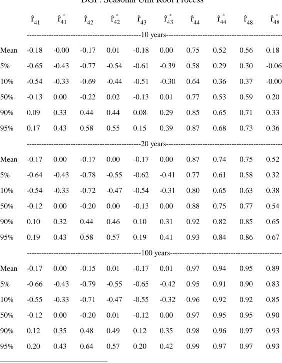
Table B.1 summarizes the simulation results for the DGP specified in (2.4) where the process contains unit roots at the seasonal frequencies as well as at the zero frequency. The striking result emerging from Table B.1 is that the ACF with seasonal means removed, i.e. has for k = 1,2,3 (i.e., non-seasonal lags) a distribution which is symmetric and centered around zero. When seasonal means are not removed, very different results emerge. Indeed, the distribution of is centered around -0.17 with a long left-tail, and hence is not symmetric. Hence, not removing seasonal means results in a strong negative bias in the ACF at non-seasonal lags. For k = 4, we find that is downward biased relative to . Yet, in moderate to large samples, the difference does not appear to be large. As the estimated ACF tends to follow the behavior of the theoretical ACF, the computed values of the sample ACF can be used to detect the presence of certain unit roots, which complements the outcome of the test results for seasonal unit roots, and hence to suggest appropriate model specification. Overall the simulations confirm that the asymptotic results in (2.5) and (2.7) hold for small and moderate sample sizes. The distributional properties of the sample ACF for seasonal dummy models are reported in Table B.2. In this case, while the behavior of the sample ACF depends on the autocorrelation structure of u process, the usual form of the sample ACF_t displays strong spikes which decay very slowly at the seasonal lags. These seasonal spikes disappear when seasonal means are removed in calculating the

autocorrelations, which is expected from the result in Theorem 2.2. In this case, it would be more sensible to remove seasonal means when we use the sample autocorrelation structure for the model identification and specification.

4 Concluding Remarks

Seasonal fluctuations are an important source of variation in economic time series, and part of the increasing interest in the treatment of seasonality in economic time series has focused on detecting the presence of unit roots at some of the seasonal frequencies as well as at the zero frequency. Yet, no clear view has emerged out of the ongoing debates on the model specification for seasonal time series. One objective of this paper is to discuss what classes of seasonal processes are responsible for the seasonality in most economic time series data, and hence to improve our understanding of seasonality and to capture it in a statistical model. In this paper, we discuss the issues concerning the model identification approach to seasonal time series data. We first investigate theoretical and practical issues on the behavior of the sample ACF in seasonal time series. In particular, two types of DGPs are considered, namely: when the process contains some roots on the unit circle, and when the process has different seasonal means.

References

Bell, W.R. and S.C. Hillmer (1984), "Issues Involved with the Seasonal Adjustment of Economic Time Series (with Comments)", Journal of Business and

Economic Statistics 2, 291-349.

Bierens, H.J. (1993), "Higher-Order Sample Autocorrelations and the Unit Root Hypothesis", Journal of Econometrics 57, 137-160.

Box, G.E.P. and G.M. Jenkins (1976), Time Series Analysis, Forecasting and

Control (Holden Day, San Francisco).

Chan, N.H. and C.Z. Wei (1988), "Limiting Distributions of Least Squares Estimates of Unstable AR Processes", Annals of Statistics 16, 367-401. Dickey, D.A. and W.A. Fuller (1979), "Distribution of the Estimators for

Autoregressive Time Series With a Unit Root", Journal of the American

Statistical Association 74, 427-431.

Dickey, D.A., H.P. Hasza and W.A. Fuller (1984), "Testing for Unit Roots in Seasonal Time Series", Journal of the American Statistical Association 79, 355-367.

Engle, R.F., C.W.J. Granger, S. Hylleberg and H.S. Lee (1993), "Seasonal Cointegration: The Japanese Consumption Function", Journal of

Econometrics 55, 275-298.

Fuller, W.A. (1976), Introduction to Statistical Time Series (Wiley, New York). Ghysels, E., H.S. Lee and J. Noh (1994), "Testing for Unit Roots in Seasonal Time

Series: Some Theoretical Extensions and a Monte Carlo Investigation",

Journal of Econometrics 62, 415-442.

Hasza, D.P. (1980), “The Asymptotic Distribution of the Sample Autocorrelations for the Integrated ARMA Process”, Journal of the American Statistical

Association 75, 349-352.

Hasza, D.P. and W.A. Fuller (1982), "Testing for Nonstationary Parameter Specifications in Seasonal Time Series Models", The Annals of Statistics 10, 1209-1216.

Hylleberg, S., R.F. Engle, C.W.A. Granger and B.S. Yoo (1990), "Seasonal Integration and Cointegration", Journal of Econometrics 44, 215-238.

Lee, H.S. (1992), "Maximum Likelihood Inference on Cointegration and Seasonal Cointegration", Journal of Econometrics 54, 1-47.

Pierce, D.A. (1978), "Seasonal Adjustment When Both Deterministic and Stochastic Seasonality are Present", in Seasonal Analysis of Economic Time

Series (ed.) by A. Zellner (U.S. Bureau of the Census), 242-273.

Phillips, P.C.B. (1987), "Time Series Regression With a Unit Root", Econometrica 55, 277-301.

T (1& ˆr_dk() ' T['

T

t'dk%1( yt& ¯y s

t ) (yt&dk& ¯y s t&dk) 'T t'1( yt& ¯y s t ) 2 ] ' T[' T t'1(yt& ¯y s t ) 2_&'T t'dk%1ytyt&dk%' T t'dk%1yt¯y s t&dk%' T t'dk%1yt&dk¯y s t &' T t'dk%1¯y s t 2 'T t'1( yt& ¯y s t ) 2 ] .

E(u_t) ' 0 for all t.

sup_t E(u_t) < 4 for some > 4.

2 _{' lim}

T64

E[T&1('T_t'1u_t)2_{] exists and} 2 _{> 0.}

{u_t}4₁ is &mixing with '4_s'1 (s)1&4/ < 4.

ˆ

r_dk(

The results in Theorem 2.1 and 2.2 hold true under similar conditions, as 3

given in Assumption 2.1 of Phillips (1987).

APPENDIX A: Proof of Theorems

In order to prove Theorems 2.1 and 2.2, we shall assume the following regularity conditions given in Bierens (1993), namely:3

Assumption A.1 (a) (b) (c) (d) Proof of Theorem 2.1

'T t'1y 2 t &' T t'dk%1ytyt&dk&' d

s'1¯ys[( ys%...%ydk&d%s)%(yT&dk%s%...%yT&d%s)] % k'd s'1¯y 2 s ' (y 2 1%...%y 2 dk)%' T

t'dk%1yt(yt&yt&dk)&' d

s'1¯ys[(ys%...%ydk&d%s) %(y_T&dk%s%...%y_T&d%s)]%k'd_s'1¯y_ts2

T (1& ˆr_dk() ' o_p(1) %

T&1'T_t'dk%1y_t( y_t&y_t&dk)&T&1'd_s'1¯y_s( y_T&dk%s%...%y_T&d%s)% T&1k'd_s'1¯y_s2

T&2'T_t'1y_t2& 1 dT &1_'d s'1¯y 2 s . T&2'T_t'1y_t2 6 2 d2' d s'1_m 1 0 W_s(r)2dr

T&1'T_t'1y_t( y_t&y_t&dk) 6 2 d k' d s'1[Ws(1) 2_% 2 dk 2] 'T t'1¯y s t 2 ' 'T t'1yt¯y s t ' T d' d s'1¯y 2 s , 'T t'1( yt& ¯y s t ) 2_{' '}T t'1y 2 t & T d' d s'1¯y 2 s,

T&1(y₁2%...%y_dk2) 6 0 and T1/2(y_s%...%y_dk&d%s) 6 0,

(A.1)

(A.2)

(A.3)

Since the denominator of the above expression

becomes

while the numerator can be rewritten as

Noting that the above

expression can be written as

The asymptotic distribution of the sample ACF in (2.7) can now be derived by using the results on the limiting distribution of the terms in (A.1), [see Chan and Wei (1988)], namely:

T&1/2¯y_s 6 d m 1 0 W_s(r)2dr for s' 1,...,d T&1/2y_T&dj%s 6 d W_s(1) for j' 1,...,k and s ' 1,..,d. n (ˆ_µd& 1) &2Wi(1)m 1 0 W_i(r)dr rˆ_dk( ˆ_µd ¯y p 6 1 d ' d s'1 s ¯y_s p 6 s T&1'T_t'1y_ty_t&k p 6 1 d ' d s'1 s s&k % k (A.4) (A.5)

Remark: It is worth noting that the expression in (2.7) is similar to the limiting distribution of in Theorem 1 of Dickey, Hasza and Fuller (1984), except for the term in the numerator. This term appears here as is obtained from the regression of y_t-dk on y , while _t is from the regression of y on_t y .t-d

Proof of Theorem 2.2

Similarly to the proof of Theorem 2.1, the distributional results in (2.13) and (2.14) can be derived by using the following relations for the time series generated by (2.8):

(A.6)

(A.7)

ˆr₄₁ ˆr₄₁( ˆr₄₂ ˆr₄₂( ˆr₄₃ ˆr₄₃( ˆr₄₄ ˆr₄₄( ˆr₄₈ ˆr₄₈( APPENDIX B: Simulation Results

Table B.1: Monte Carlo Simulations Autocorrelation Functions DGP: Seasonal Unit Root Process

---10 years---Mean -0.18 -0.00 -0.17 0.01 -0.18 0.00 0.75 0.52 0.56 0.18 5% -0.65 -0.43 -0.77 -0.54 -0.61 -0.39 0.58 0.29 0.30 -0.06 10% -0.54 -0.33 -0.69 -0.44 -0.51 -0.30 0.64 0.36 0.37 -0.00 50% -0.13 0.00 -0.22 0.02 -0.13 0.01 0.77 0.53 0.59 0.20 90% 0.09 0.33 0.44 0.44 0.08 0.29 0.85 0.65 0.71 0.33 95% 0.17 0.43 0.58 0.55 0.15 0.39 0.87 0.68 0.73 0.36 ---20 years---Mean -0.17 0.00 -0.17 0.00 -0.17 0.00 0.87 0.74 0.75 0.52 5% -0.64 -0.43 -0.78 -0.55 -0.62 -0.41 0.77 0.61 0.58 0.32 10% -0.54 -0.33 -0.72 -0.47 -0.54 -0.31 0.80 0.65 0.63 0.38 50% -0.12 0.00 -0.20 0.00 -0.13 0.00 0.88 0.75 0.77 0.54 90% 0.10 0.32 0.44 0.46 0.10 0.31 0.92 0.82 0.85 0.65 95% 0.19 0.43 0.58 0.57 0.19 0.41 0.93 0.84 0.86 0.67 ---100 years---Mean -0.17 0.00 -0.15 0.01 -0.17 0.01 0.97 0.94 0.95 0.89 5% -0.66 -0.43 -0.79 -0.55 -0.65 -0.42 0.95 0.91 0.90 0.83 10% -0.55 -0.33 -0.71 -0.47 -0.55 -0.32 0.96 0.92 0.92 0.85 50% -0.12 0.00 -0.20 0.01 -0.12 0.00 0.97 0.95 0.95 0.90 90% 0.12 0.35 0.48 0.49 0.12 0.35 0.98 0.96 0.97 0.93 95% 0.20 0.43 0.64 0.57 0.20 0.42 0.99 0.97 0.97 0.93 ___________________________

Notes: The data generating process is: y = y + u , where u is i.i.d. standard normal. Thet t-4 t t

Monte Carlo simulations involved 10000 replications. The autocorrelations r , k = 1, 2,^ 4k

3, 4 and 8 are defined in (2.1) and use the unconditional sample mean while the r_4k*

autocorrelations involve seasonal means. They are defined in (2.6). Entries to the table are the Monte Carlo distribution mean and percentiles.

ˆr₄₁ ˆr₄₁( ˆr₄₂ ˆr₄₂( ˆr₄₃ ˆr₄₃( ˆr₄₄ ˆr₄₄( ˆr₄₈ ˆr₄₈(

y_t ' 'd_{s'1 s}D_st% u_t,

r_4k(

Table B.2: Monte Carlo Simulations Autocorrelation Functions DGP: Seasonal Dummies Process

---10 years---Mean -0.50 -0.00 0.46 -0.01 -0.47 0.00 0.44 -0.10 0.39 -0.10 5% -0.69 -0.27 0.24 -0.26 -0.66 -0.26 0.22 -0.33 0.19 -0.32 10% -0.65 -0.21 0.29 -0.20 -0.62 -0.20 0.27 -0.29 0.24 -0.26 50% -0.51 0.00 0.46 -0.01 -0.48 0.00 0.45 -0.10 0.39 -0.10 90% -0.33 0.20 0.61 0.18 -0.31 0.21 0.59 0.09 0.53 0.08 95% -0.29 0.26 0.65 0.25 -0.25 0.26 0.62 0.14 0.56 0.13 ---20 years---Mean -0.50 0.00 0.48 0.00 -0.48 0.00 0.47 -0.05 0.45 -0.05 5% -0.64 -0.20 0.33 -0.18 -0.62 -0.18 0.32 -0.23 0.30 -0.22 10% -0.61 -0.15 0.37 -0.13 -0.59 -0.14 0.35 -0.19 0.34 -0.18 50% -0.51 0.00 0.49 0.00 -0.49 0.00 0.48 -0.05 0.45 -0.05 90% -0.38 0.15 0.59 0.14 -0.37 0.14 0.58 0.09 0.55 0.09 95% -0.35 0.19 0.62 0.19 -0.34 0.18 0.61 0.13 0.58 0.12 ---100 years---Mean -0.50 0.00 0.50 0.00 -0.50 0.00 0.49 0.00 0.49 -0.01 5% -0.56 -0.08 0.43 -0.08 -0.56 -0.08 0.43 -0.09 0.42 -0.09 10% -0.55 -0.06 0.45 -0.06 -0.55 -0.06 0.44 -0.07 0.44 -0.07 50% -0.50 0.00 0.50 0.00 -0.50 0.00 0.49 -0.01 0.50 -0.01 90% -0.45 0.06 0.54 0.06 -0.45 0.06 0.54 0.05 0.54 0.06 95% -0.44 0.08 0.56 0.08 -0.43 0.08 0.56 0.07 0.55 0.07 ___________________________

Notes: The data generating process is where u is i.i.d. standardt

normal. The seasonal mean shifts are =-1 for s = 1, 3 and = 1 for s = 2, 4. The Montes s

Carlo simulations involved 10000 replications. The autocorrelations r , k = 1, 2, 3, 4 and^ 4k

8 are defined in (2.1) and use the unconditional sample mean while the autocorrelations involve seasonal means. They are defined in (2.6). Entries to the table are the Monte Carlo distribution mean and percentiles.

Vous pouvez consulter la liste complète des publications du CIRANO et les publications %

elles-mêmes sur notre site World Wide Web à l'adresse suivante :

http://www.cirano.umontreal.ca/publication/page1.html

Liste des publications au CIRANO %

Cahiers CIRANO / CIRANO Papers (ISSN 1198-8169)

96c-1 Peut-on créer des emplois en réglementant le temps de travail ? / Robert Lacroix 95c-2 Anomalies de marché et sélection des titres au Canada / Richard Guay, Jean-François

L'Her et Jean-Marc Suret

95c-1 La réglementation incitative / Marcel Boyer

94c-3 L'importance relative des gouvernements : causes, conséquences et organisations alternative / Claude Montmarquette

94c-2 Commercial Bankruptcy and Financial Reorganization in Canada / Jocelyn Martel 94c-1 Faire ou faire faire : La perspective de l'économie des organisations / Michel Patry

Série Scientifique / Scientific Series (ISSN 1198-8177)

97s-35 Seasonal Time Series and Autocorrelation Function Estimation / Hahn Shik Lee, Eric Ghysels et William R. Bell

97s-34 Do Canadian Firms Respond to Fiscal Incentives to Research and Development? / Marcel Dagenais, Pierre Mohnen et Pierre Therrien

97s-33 A Semi-Parametric Factor Model of Interest Rates and Tests of the Affine Term Structure / Eric Ghysels et Serena Ng

97s-32 Emerging Environmental Problems, Irreversible Remedies, and Myopia in a Two Country Setup / Marcel Boyer, Pierre Lasserre et Michel Moreaux

97s-31 On the Elasticity of Effort for Piece Rates: Evidence from the British Columbia Tree-Planting Industry / Harry J. Paarsch et Bruce S. Shearer

97s-30 Taxation or Regulation: Looking for a Good Anti-Smoking Policy / Paul Leclair et Paul Lanoie

97s-29 Optimal Trading Mechanisms with Ex Ante Unidentified Traders / Hu Lu et Jacques Robert

97s-28 Are Underground Workers More Likely To Be Underground Consumers? / Bernard Fortin, Guy Lacroix et Claude Montmarquette

97s-27 Analyse des rapports entre donneurs d’ordres et sous-traitants de l’industrie aérospatiale nord-américaine / Mario Bourgault

97s-26 Industrie aérospatiale nord-américaine et performance des sous-traitants : Écarts entre le Canada et les États-Unis / Mario Bourgault

97s-25 Welfare Benefits, Minimum Wage Rate and the Duration of Welfare Spells: Evidence from a Natural Experiment in Canada / Bernard Fortin et Guy Lacroix