Bramoullé: Département d’économique, Université Laval and CIRPÉE
Kranton: Duke University
D’Amours: Département d’économique, Université Laval
We dedicate this paper to the memory of Toni Calvó-Armengol. As will be clear in the subsequent pages, he has made a lasting contribution to our thinking about networks and economics. We deeply miss his insight and his company. We are grateful to Alexander Groves for research assistance and to Noga Alon, Roland Bénabou, Francis Bloch, Andrea Galeotti, Sanjeev Goyal, Matthew Jackson, Antoine Loeper, Brian Rogers, and Yves Zenou and participants in seminars and conferences at Barcelona, Berkeley, Caltech, Cambridge, Duke, École Polytechnique (Paris), Essex, MEDS (Northwestern), Laval (Québec), Montréal, NYU Stern School, Paris School of Economics, and Stockholm for helpful comments and discussions. For support, Rachel Kranton thanks the Canadian Institute for Advanced Research, and Yann Bramoullé thanks the Social Sciences and Humanities Research Council and the Canada Research Chair in Social Policies and Human Resources.
Cahier de recherche/Working Paper 10-18
Strategic Interaction and Networks
Yann Bramoullé
Rachel Kranton
Martin D’Amours
Abstract:
This paper brings a general network analysis to a wide class of economic games. A
network, or interaction matrix, tells who directly interacts with whom. A major challenge
is determining how network structure shapes overall outcomes. We have a striking
result. Equilibrium conditions depend on a single number: the lowest eigenvalue of a
network matrix. Combining tools from potential games, optimization, and spectral graph
theory, we study games with linear best replies and characterize the Nash and stable
equilibria for any graph and for any impact of players’ actions. When the graph is
sufficiently absorptive (as measured by this eigenvalue), there is a unique equilibrium.
When it is less absorptive, stable equilibria always involve extreme play where some
agents take no actions at all. This paper is the first to show the importance of this
measure to social and economic outcomes, and we relate it to different network link
patterns.
Keywords: Networks, potential games, lowest eigenvalue, stable equilibria, asymmetric
equilibria
I. Introduction
In many economic settings, people and …rms do not interact equally and directly with everyone. A network, or interaction matrix or graph, can formally capture various cross-cutting links and relationships by indicating whose actions directly a¤ect whose payo¤s. The matrix can represent social links, geography, agents’preferences, market structure, or information ‡ows. Because linked players interact with other linked players, outcomes depend on the entire network structure. The major challenge and interest is determining how network structure shapes outcomes. Networks are complex objects and answering this question is generally di¢ cult even in otherwise simple settings. We study strategic interaction and networks for an important class of games— games with linear best replies. Such games have been used to study a wide variety of settings including public goods, oligopoly, resource extraction, criminal activity, investment, belief formation, and peer e¤ects.1 We bring to bear a new combination of tools and characterize the Nash and stable equilibria for any graph structure and for any impact of players’actions on others’payo¤s.
We have a striking result. Using tools from potential games, optimization, and spectral graph theory, we …nd that equilibrium outcomes depend on a single number: the lowest eigenvalue of a network matrix. When the network matrix is su¢ ciently absorptive (as measured by this eigenvalue), there is a unique equilibrium. An equilibrium is stable when the graph connecting active agents is su¢ ciently absorptive (as measured by the lowest eigenvalue). This paper is the …rst to show the importance of this measure to social and economic outcomes, and we relate it to patterns of network links.2
While our …ndings hold in general, we focus on games of strategic substitutes. Strategic substi-tutes settings include oligopoly interaction, public good provision, research & development, price and information-gathering by consumers, and experimentation with new technologies.3 Strategic
substitute games involve complexities not present with strategic complements. Agents’ actions tend to go in opposite directions. There are often multiple equilibria, which cannot generally be neatly ordered. To tackle multiple equilibria, we consider stable equilibria as a subset of Nash
1
See, for example, Angeletos & Pavan (2007), Ballester, Calvó-Armengol & Zenou (2006), Bergemann & Morris (2009), Calvó-Armengol, Patacchini & Zenou (2009), Bénabou (2008), Bramoullé & Kranton (2007), ·Ilkiliç (2008), Glaeser & Scheinkman (2003), Goyal & Moraga-González (2001), and Vives (1999).
2
For a compendium of network measures, see Wasserman & Faust (1994) and Scott (2004). Echenique & Fryer (2007), for example, use the highest eigenvalue as a measure of segregation.
3
equilibria. Stable equilibria are robust to small changes in agents’play.4 We …nd an equilibrium is stable when the graph connecting active agents has large absorptive capacity (measured by the lowest eigenvalue) relative to the impact of play. We also …nd that, except for small payo¤ impacts, stable equilibria always involve asymmetric and extreme outcomes— some players do nothing at all. Thus the common restriction of attention in the literature to symmetric equilibria can be misleading. To tackle comparative statics, we use our combination of tools to show when for stable equilibria, and overall, aggregate actions decrease. Thus, for example, an additional link in a network can decrease the total provision of public goods.5
From these results the paper builds general intuitions about strategic play in networks. First, even when agents have symmetric network positions, play is likely to be concentrated on a few players. Interior and symmetric outcomes are the exception rather than the norm. Second, while there is a rich variety of equilibria, there is a tight relation between the structure of the equilibrium set and the shape of the overall network. The lowest eigenvalue gives a critical measure of this relation. Third, this mathematical index relates to the geometry of the network. It captures partitions of society into distinct sets. When individuals have fewer links within sets and more links between sets, the system tends to amplify payo¤ impacts and to reach corner outcomes.
This paper makes at least three contributions.
First, this paper advances the analysis of n-person simultaneous-move games with continuous action spaces. As mentioned above, there is a wide variety of applications that are modeled with payo¤s that have linear best responses. The canonical game is one with quadratic payo¤s. Often researchers restrict attention to (a) the case where all agents interact equally with all other agents, (b) symmetric equilibria, and (c) interior equilibria. This paper gives the tools to study any possible interaction structure, the entire action space, and the full set of equilibrium outcomes.6 New conclusions are then possible, such as comparative statics and how equilibria relate to network structure.
Second, we advance the recent and active literature on games played on networks. This paper
4Formally, we consider asymptotically stable equilibria. Given a system of linear di¤erential equations de…ned
using agents’best response functions, an equilibrium is stable when the system converges back to the equilibrium following any small enough perturbation in agents’actions.
5
Bramoullé & Kranton (2007) contains a special case of this result, and Bloch & Zenginobuz (2007) show spillovers can lead to lower public good provision.
6
For instance, our approach can be used to study the leading public goods example in Bergemann & Morris (2008, 2009) for an arbitrary network.
integrates and supercedes …ndings in two main lines of inquiry. In this previous work, games have quite di¤erent payo¤ functions, but— as we point out here— best-response functions are identical and linear. Ballester, Calvó-Armengol & Zenou (2006) study a quadratic-payo¤ game where agents are harmed by other agents’ actions. They examine outcomes when agents have weak impacts on others, identifying a su¢ cient condition for a unique, interior, equilibrium. In this equilibrium agents’actions are proportional to their Bonacich centrality measures.7 Bramoullé & Kranton (2007) study a game where agents gain from other agents’actions. The analysis examines the opposite end of the spectrum, when agents have strong impacts on others (actions are perfect substitutes). Multiple equilibria are the rule, and there is always an equilibrium where some individuals choose an action of zero. These specialized equilibria involve maximal independent sets of the network graph. The present paper analyzes the full range of impacts— agents’impacts on others ranges from weak to strong— for any graph. We identify a precise relationship between graph structure, payo¤ impacts, and unique and stable equilibria.
With these …ndings, we also make signi…cant progress on the problems of multiplicity of equilibria and comparative statics in network settings. Researchers in this area are often frustrated by the large number of equilibria and the di¢ culty of characterizing and comparing equilibria. Galeotti, Goyal, Jackson, Vega-Redondo & Yariv (2009) explore how to overcome these issues by assuming players have limited information about the graph structure. They obtain sharp analytical results for symmetric equilibria. In the present paper, we take a more traditional approach; agents play a simultaneous move game on a graph, and we explore Nash and stable equilibria. To attack characterizing equilibria and comparative statics, we use di¤erent tools and concepts such as potential functions and structural network features.
Third, the paper connects traditional economics techniques and outcomes to traditional com-puter science. We characterize equilibrium outcomes as solutions to well-de…ned quadratic pro-gramming problems. We construct an (necessarily exponential time) algorithm to identify all equilibria and show that solving for certain focal equilibria is directly related to a well-known NP hard problem. We exploit Monderer & Shapley’s (1996) theory of potential games that computer scientists have used to study congestion and other issues (e.g., Roughgarden & Tardos (2002),
7Ballester, Calvó-Armengol & Zenou (2006) are the …rst to make the connection between centrality measures
and strategic play. In a similar game, Ballester & Calvó-Armengol (2007) …nd a su¢ cient condition for a unique equilibrium. Corbo, Calvó-Armengol & Parkes (2007) study network design in the same setting.
Chien & Sinclair (2007)). In economics, the theory of potential games has been applied to …nite games, including a few network settings.8 Neyman (1997) studies potential games with continuous actions and …nds conditions for a unique correlated equilibrium. We provide the …rst application to network games with a continuous action space. We show how to use it, in combination with other tools, to illuminate strategic interaction in networks. These cross-overs could have great impact on overall study of networks and multiple player games.
The paper proceeds as follows. In the next section we present the model and give our basic characterization of Nash equilibria. Section III …nds the relationship between the lowest eigen-value of the network matrix and unique and corner equlibria. We study stable equilibria in Section IV. Section V connects the lowest eigenvalue to network link patterns. We conduct comparative statics in Section VI. We show how our results generalize and apply to many more games in Section VII and conclude in Section VIII.
II. Class of Games and Nash Equilibria A. The Model
We present the basic model here. The results extend generally as described in Section VII. There is a set of n agents denoted N . Each agent i simultaneously chooses an action xi 2
[0; 1): Let x denote an action vector for all agents and x i denote an action vector of all agents
other than i. To specify payo¤s, we use a graph, or network, or interaction matrix, which is an n n matrix G = [gij],9 where gij = 1 if i impacts j’s payo¤s directly, gij = 0 otherwise, and it
is assumed gij = gji.10 We set gii= 0. Following common usage, we say agent i and j are linked,
connected, or neighbors when gij = gji= 1. Payo¤s are
Ui(xi; x i; ; G);
where 2 R is the payo¤ impact parameter; i.e., how much i’s neighbors a¤ect Ui. Let xi be the
action individual i would take in isolation; xi maximizes Ui when = 0 or gij = 0 for all j:
8Blume (1993) studies …nite games when players are situated on a lattice. Young (1998) considers coordination
games with two actions and general networks. Bramoullé (2007) studies anti-coordination games with two actions and general networks.
9
Throughout the paper, we identify a network with its adjacency matrix.
1 0
For the basic model, 2 [0; 1] which, in combination with gij 0, will yield strategic
substi-tutes. Our results apply to the less complicated setting of strategic complements, where 0 or gij 0, contained in Section VII, along with mixed strategic substitutes and complements.11
B. Class of Games: Payo¤s with Linear Best Replies
We study games where payo¤ functions have di¤erent functional forms but all have the same linear best reply functions. As discussed, canonical games in economics and the network literature fall in this class. We …nd pure-strategy Nash and stable equilibria.12 Since the games have the same best reply functions, the games have the same set of equilibrium outcomes.
We …rst present three exemplary games in this class. We then fully describe the best-reply functions. In each of the games that follow xi = x for all i. This will be the base case, and the
results hold generally as discussed in Section VII.
The …rst game is a model of public goods in networks (Bramoullé & Kranton (2007)). Indi-vidual i bene…ts from his own and his neighbors’actions, and indiIndi-vidual i’s payo¤ is
b
Ui(xi; x i; ; G) = b(xi+
X
j
gijxj) xi;
where b(:) is strictly increasing and strictly concave on R+, and > 0 is the constant marginal
cost of own action, such that b0(0) > > b0(+1). As in Bergstrom, Blume & Varian (1986), public goods are privately provided, but here public goods are local. Bramoullé & Kranton (2007) primarily study the case of = 1 (i’s neighbors’actions are perfect substitutes for xi).
The second game is from Ballester, Calvó-Armengol & Zenou (2006) where agents are hurt, not helped, by neighbors. Individual i’s payo¤ is
e Ui(xi; x i; ; G) = xxi 1 2x 2 i X j gijxixj:
For future reference, we call eUi quadratic payo¤ s. Ballester, Calvó-Armengol & Zenou (2006) and
1 1
Thus our analysis readily accomodates local complementarities and global substitutabilities as in Ballester, Calvó-Armengol & Zenou’s (2006) general model. The graph G would give the net of the complements and substitutes for each ij: That is, G C L, where and are positive parameters, C is the complete graph, and in graph L lij= lji 0for all ij and lii= 0for all i.
1 2
Ballester & Calvó-Armengol (2007) study this game for low.
The third game is a standard di¤erentiated-product Cournot oligopoly with linear (inverse) de-mand and constant marginal cost.13 With marginal cost d, …rm i facing demand Pi(xi; x i; ; G) =
a b (xi+ 2 Pjgijxj) has payo¤s: i(xi; x i; ; G) = xi 0 @a b (xi+ 2 X j gijxj) 1 A dxi;
where gij = 1 indicates i and j’s products are substitutes and captures the degree of
substi-tutability. Vives (1999) considers interior equilibria.
In these three games agent i has the same best response function:
xi = x X j gijxj if X j gijxj < x and (1) xi = 0 if X j gijxj x:
Agent i will achieve x through his own and his neighbors’ actions. If the weighted sum of neighbors’actions is less than x, agent i makes up the di¤erence. If the weighted sum is higher than x, agent i chooses 0. Without loss of generality, normalize x 1 to yield the best reply function fi(x) 2 [0; 1]: fi(x; ; G) = max(0; 1 n X j=1 gijxj): (2)
We solve for the Nash equilibria and stable equilibria for games with this best-reply. A Nash equilibrium is a vector x 2 [0; 1]nthat simultaneously satis…es xi = fi(x; ; G) for all agents i 2 N.
A Nash equilibrium could be unstable in the sense that a small change in actions could lead— through an adjustment process— to a di¤erent action vector. We study a continuous adjustment process and …nd asymptotically stable equilibria.14
Our objective is to solve for and characterize all Nash equilibria and all stable equilibria as they depend on the payo¤ parameter and on the graph G. Throughout the paper, for a given
1 3
Linear inverse demand functions derive from consumers with strictly concave quadratic utility functions (Vives (1999)).
1 4
We thus follow early work on Cournot games with multiple sellers (Fisher (1961)) that shows existence of stable equilibria with continuous but not discrete adjustment— a …nding replicated here.
graph G we say that a property holds for almost every if it holds for every except possibly a …nite number of values.15
We use the following terminology and notation. We say a vector x is interior if 8i; xi > 0. A
vector x is a corner if for some agent i; xi = 0: A corner vector x is specialized if 8i; xi 2 f0; 1g.
Let I denote the n-square identity matrix, let 1 denote a vector of ones, o a vector of zeros, and O a square matrix of zeros. The empty network is then G = O. In a complete network, denoted by C; every agent is connected to every other agent.
For individual agents, let ki denote the number of i’s neighbors, called i’s degree; ki =Pjgij.
Let kmin(G) and kmax(G) respectively, denote the smallest and largest degree in graph G. For
an agent’s centrality, given a graph G and a scalar q such that I qG is invertible, the vector of Bonacich centralities c(q; G) is de…ned by c(q; G) = (I qG) 1G1 (Bonacich (1987)). The centrality measure for agent i, ci(q; G); can be seen as a weighted sum of the paths in G that
start with i.16
For overall graph structure, let min(G) and max(G) denote the lowest and highest
eigenval-ues of G, respectively, and let (G) max(j min(G)j; j max(G)j) denote its spectral radius.
The value min(G) features prominently in our results. Since any graph G is square and
symmetric, min(G) 0 and max(G) 0. Furthermore, max(G) min(G).17 For a higher
min(G), we say the graph has more absorptive capacity. We will see that an absorptive graph
dampens— rather than magni…es— the impact of players’actions captured in :
C. Complete Set of Nash Equilibria
Existence of Nash equilibria is guaranteed thanks to a …xed-point argument.18 The equilibrium set has been well-studied when is low (Ballester, Calvó-Armengol & Zenou (2006)) and when
= 1 (Bramoullé & Kranton (2007)). Little has been known for the general case.
Our …rst proposition gives the general characteristics of pure strategy Nash equilibria for any and G: For a vector x, let A denote the set of active agents— those agents whose actions are
1 5For a graph G, the set of values for which the property does not hold has zero measure. 1 6
When jqj is su¢ ciently small, c(q; G) = G1 + qG21+ q2G31+ , and paths of length k are weighted by qk 1.
1 7
For any square matrix, the sum of the eigenvalues is equal to its trace. For any symmetric matrix, all eigenvalues are real numbers. Since G is a nonnegative matrix, max(G) min(G)by Perron’s theorem (see Theorem 0.13
in Cvetkovi´c et al. (1979)).
1 8
strictly positive: A = fi : xi> 0g. Agents outside this set are called inactive agents. Let xA
denote the action vector of active agents; let GAdenote the subgraph of G connecting the active
agents; and let GN A;A denote the graph of links connecting active agents to inactive agents.
Parsing the network in this way and using matrix notation to express the best-reply conditions in (2) leads directly to the following result.
Proposition 1. A pro…le x with active agents A is a Nash equilibrium if and only if
(1) (I + GA)xA = 1
(2) GN A;AxA 1
From Proposition 1 we have several direct …ndings.19 First, we can compose a simple algorithm to …nd all the equilibria for any graph G and almost every : Given a graph G, consider a subset S N . If det(I + GS) 6= 0, compute the pro…le xS = (I + GS) 11 and set xN S = o. Check
whether xS 0 and GN S;SxS 1. If these two sets of linear inequalities are satis…ed, x is an
equilibrium. If either condition fails, it is not. Repeating this procedure for every subset of N yields all the equilibria for G and almost every .20 Second, for any graph G and almost every
, the equilibria are …nite,21 since for a given graph G, 8S, det(I + GS) 6= 0 for almost every .
Third, we see how individual equilibrium play relates to graph position. Comparing two agents whose neighbors are nested sets, for < 1 the agent with the larger set of neighbors plays less. Intuitively, an agent who is linked to more outside sources can take a lower action. In addition, all equilibria for any G and almost every can be described by the vector of individual Bonacich centralities in GA. For an equilibrium x; simply invert the matrix I + GA. We
then have equilibrium actions xA = (I + GA) 11= 1 c( ; GA), and for active player i,
xi= 1 ci( ; GA).22 Thus, we validate here Bonacich’s (1987) original insight on the impact
1 9See Appendix for proofs. 2 0
Any such algorithm must run in exponential time since the number of equilibria is potentially exponential. In the language of computer science, our algorithm is “a total enumeration method,” and researchers have been looking for “partial enumeration methods”for such problems (Murty & Yu (1988)). We have derived several results (available upon request) that help identify the active set of agents, and thus could reduce computational time. First, using the fact that f f is increasing, we obtain a lower bound on individual actions in any equilibrium. This yields a computationally fast procedure to determine agents who are active in all equilibria. Second, for the vector xs= (I + GS) 11, removing those agents for whom xi 0can yield the set A of active agents.
2 1
Even when not …nite, the equilibrium set has a well-de…ned mathematical structure. For any and G the set of equilibria is a …nite union of compact convex sets.
2 2Write (I + G
of a negative scalar (here ) on his measure. With a negative scalar, an agent’s Bonacich centrality tends to be higher when linked to agents who themselves have few neighbors. These agents then choose lower actions.
Proposition 1 yields equilibria for all 2 [0; 1] and supercedes previous …ndings for low and = 1. We brie‡y review here the previous results, as written in the notation of the present paper. Low : Using the theory of positive matrices, Ballester, Calvó-Armengol & Zenou (2006, Theorem 1) show that if < 1=(1 + max(C G)), there is a unique interior equilibrium where
agents’actions can be described by their Bonacich centralities in the graph C Gfor the scalar =(1 ).23 For future reference, we label this critical value as BCAZ 1=(1 + max(C G)).
High : Using graph theory, Bramoullé & Kranton (2007, Theorem 1) show for = 1, spe-cialized equilibria exist for any non empty graph. The active players in these equilibria constitute a maximal independent set of the graph G.24 For < 1; specialized equilibria relate to maximal independent sets where inactive agents are connected to at least 1= agents in the set.
The following examples illustrate our results with canonical network structures and highlight the advances over previous work, showing the equilibria for the full range of .
Figure 1: Equilibria in a Star Network
2 3
Decomposing the network as G = C (C G) ;where C captures global substitutes and (C G)captures local complements, and introducing the vector y = 1 +1 c 1 ; C G , their result states that if < 1=(1 +
max(C G));the unique equilibrium action vector is x =1 +1P
jyjy, which is interior.
2 4
A set of agents I is an independent set of the graph G if for all i; j 2 I; gij= 0. An independent set I is maximal
if I is not a subset of another independent set. Given any maximal independent set, agents in the population are divided into (i) those in the set and (ii) those linked to an agent in the set.
Example 1. Stars. Consider a star with n players. Figure 1, for n = 4, shows, for < BCAZ = 1=(n 1) the unique, interior, equilibrium where the center plays [1 (n 1) ]=[1 (n 1) 2] and each peripheral agent plays (1 )=[1 (n 1) 2]. For = 1, there are two specialized equilibria: (i) the center plays 0 and peripheral agents play 1, and (ii) the center plays 1 and the peripheral agents play 0: For the middle range, 1=(n 1) < 1, there is a unique equilibrium. It is specialized; the center plays 0 and peripheral agents play 1. The star graph thus shows that unique equilibria can exist above BCAZ, and the unique equilibrium need not be interior.
Figure 2: Equilibria in a Line Network
Example 2. Line with Four Players. Figure 2 shows for < BCAZ ' 0:382 the unique, interior, equilibrium where players 1 and 4 on the ends play 1
1+ 2, and players 2 and 3 in the
middle play 1+1 2. For = 1, there are multiple equilibria, and the …gure shows one specialized
outcome where active agents are a maximal independent set of the graph. For the middle range of , there is a unique equilibrium, which is interior, for BCAZ < < min(G) =
p 5 1 2 ' 0:618. For p 5 1
2 < < 1, two corner equilibria emerge in addition to the interior one. To preview later
results, in this range only the corner equilibria are stable. This example shows that an interior equilibrium can exist for any value of , and it may not be unique or stable.
Example 3. Complex network. Figure 3 depicts equilibria on a complex network linking 20 agents. This network is a particular realization of a Poisson random graph with connection probability of 0:75. Agents with more links are depicted closer to the center, and a node’s color is proportional to its action on a Black-White scale (Black=1, White=0). We see for < BCAZ ' 0:153, the unique equilibrium, which is interior. For the middle range of , we show
(a) δ = 0.15, unique equilibrium (b) δ = 0.35, 3 equilibria (c) δ = 0.55, 31 equilibria
Figure 3: Equilibria in a Complex Network
one of the three equilibria for = 0:35 and one of the thirty-one equilibria for = 0:55.25 At = 0:35, many agents are inactive. At = 0:55, the equilibrium is specialized. This example shows the multiplicity and variety of equilibria for intermediate values of :
III. The Shape of Nash Equilibria
We now address the major challenge: how network structure shapes equilibrium outcomes. We derive su¢ cient conditions and necessary conditions for unique, interior, corner, and stable outcomes— all as functions of the network structure and payo¤ parameter : We also address comparative statics, a well-known problem in the analysis of strategic substitutes games. To do so, we combine tools from the theory of potential games, the theory of maximization, and spectral graph theory.
We …nd the lowest eigenvalue of a graph, min(G), is key to equilibrium outcomes. This
result is all the more remarkable because we also show that generally …nding all equilibria is a computationally complex problem (requiring exponential time). We show that when a graph has a high min(G), the equilibrium is unique. An equilibrium is stable if and only if min(GA) is
su¢ ciently high.
These results are the …rst to reveal the signi…cance of the lowest eigenvalue of a network graph. It is not a common measure in sociology or physics, for example, and there is only a small amount of mathematical work recently on the relationship between the link structure and the lowest eigenvalue.26 Below we describe and formally elaborate this relationship. To develop an intuition, note that min(G) < 0; hence when it is smaller, it corresponds to a larger number
in absolute value. When min(G) is small, the graph contains many links that connect distinct
sets of agents— actions then have greater impact on others’play, and we say the graph has low absorptive capacity. Thus, large min(G) is key to stable outcomes.
A. Tool: Potential Function
We begin by using the theory of potential games to reformulate the equilibrium conditions. Consider a game where player i chooses xi 2 Xi, X =
Y
i
Xi, and payo¤s are Vi(xi; x i): From
Monderer & Shapley (1996), a function '(xi; x i) is a potential function for this game if and only
if for all i
'(xi; x i) '(x0i; x i) = Vi(xi; x i) Vi(x0i; x i) for all xi; x0i 2 Xi and all x i2 X i
For xi2 R and continuous, twice-di¤erentiable payo¤s Vi, there exists a potential function if and
only if @2Vi(x)
@xi@xj =
@2V i(x)
@xj@xi for all i 6= j.
Examining the game with quadratic payo¤s eUi, it has a potential function since @
2Ue i @xi@xj = gij = @ 2Ue i
@xj@xi. The following function
'(x; ; G) = n X i=1 xi 1 2x 2 i 1 2 n X i=1 n X j=1 gijxixj
is a potential function for eUi; @ e@xUii = @x@'i: Notice that '(x; ; G) is strictly concave in each xi.
We can use this potential function to …nd the equilibria for all games in our class, since all the games have the same equilibria as the game with payo¤s eUi.27 Consider the following constrained
optimization problem (P):
2 6See Desai & Rao (1994), Alon & Sudakov (2000), Ye, Fan & Liang (2008), Bell, Cvetkovi´c, Rowlinson & Simi´c
(2008a, 2008b), Trevisan (2009).
2 7
In the terminology of Morris & Ui (2004), the games in our class are “best-response potential games,” since they are “best-response equivalent” and one of the games is a potential game.
max
x '(x; ; G) s.t. 8i; xi 0; (P)
and consider the Kuhn-Tucker conditions, such as for xi
@' @xi = 0 and xi > 0; or @' @xi 0 and xi = 0:
The Kuhn-Tucker condition for each xi exactly correspond to an agent i’s individual best response
(2).28 Thus we have:
Lemma 1. A pro…le x is a Nash equilibrium of any game with the best reply function fi(x) =
max(0; 1 Pnj=1gijxj) if and only if x satis…es the Kuhn-Tucker conditions of problem (P).
The set of Nash equilibria for a given G and is then equal to the local and global maxima and saddle points of the potential function '(x; ; G) on Rn+.
Solving for the Nash equilibria for these games is then a quadratic programming problem. To see this clearly, rewrite the potential function as '(x; ; G) = xT1 12xT(I + G)x. Quadratic optimization has been well-studied in mathematics and computer science (e.g. Lee, Tam & Yen (2005)). The heart of the problem is the matrix I+ G: When I+ G is positive de…nite, '(x; ; G) is concave, there is a unique solution to (P), and (P) is solvable in polynomial time. In general, however, solving the problem (P) is NP-complete (Pardalos & Vavasis (1991)) and …nding all the maxima and saddle points requires exponential time.29 Yet knowledge about this problem gives us enormous tractability to characterize equilibria, as we discuss next.
B. Lowest Eigenvalue of Graph and Nash Equilibria
B.1. Unique Equilibria: Convex Optimization— min(G) is large
We …rst obtain a strong, intuitive condition for the uniqueness of equilibria which is the strongest in the literature. A traditional uniqueness condition derives from contraction of the best reply function, which occurs if and only if < 1= (G) (see Appendix). Thus, from standard arguments
2 8'(x
i; x i)is strictly concave in each xi;so for any x ia single xisatis…es the ithKuhn-Tucker condition. 2 9
While computer scientists have developed many algorithms that would quickly identify one equilibrium, only enumerative methods are guaranteed to …nd them all (Murty & Yu (1988)).
a unique equilibrium exists if < 1= (G):30 Our next result shows that this su¢ cient condition is not necessary. Our condition relies on min(G) and holds even when the best replies are not
contracting.
The major insight is that individual responses to others’actions are geometrically structured by the potential function. The whole action pro…le moves along the surface of the potential. It is the curvature of the potential function, and the network which gives the potential its shape which determines the number and character of equilibrium outcomes.
We …nd that the lowest eigenvalue of a graph, min(G), captures the relevant shape of the
potential. The potential function '(x; ; G) is strictly concave if and only if < 1= min(G).
This follows from the Hessian of the potential which is equal to r2' = (I + G), and I + G is positive de…nite if and only if < 1= min(G): We can then invoke the theory of convex
optimization (as applied to quadratic programming) to analyze problem (P). If '(x; ; G) is strictly concave, there is a unique global maximum, for which the Kuhn-Tucker conditions are necessary and su¢ cient.31 Thus, we have
Proposition 2. If < 1= min(G), there is a unique Nash equilibrium.
This condition is often both necessary and su¢ cient for a unique equilibrium.32 For example, it is necessary and su¢ cient for an important class of graphs, regular graphs (we show this below). We can also see necessity and su¢ ciency in particular graphs, such as the line with four players in Example 2, where min(G) =
p 5 1
2 .
Proposition 2 provides the best known su¢ cient condition for unique equilibria in these games. It is stronger than the two previous conditions: Ballester & Calvó-Armengol (2007, Proposition 1) show that there exists a unique equilibrium if < 1= (G), which corresponds to the condition for contracting best replies. For any G, 1= min(G) 1= (G); and this inequality is strict when
no component of G is bipartite.33 Ballester, Calvó-Armengol & Zenou (2006, Theorem 1) show there exists a unique interior equilibrium for < 1=(1 + max(C G)): For any G, 1= min(G)
3 0
Ballester & Calvo-Armengol (2007)) also show there is a unique equilibrium if < 1= (G) by using the mathematics of linear-complementarity problems.
3 1The result is a network case of Neyman’s (1997) …nding for general potential games with convex compact action
spaces that shows there is a unique correlated equilibrium when the potential is strictly concave. Bergemann & Morris (2007) generalize this …nding to games of incomplete information.
3 2
In addition, we know that the unique equilibrium varies continuously with when < 1= min(G). 3 3See Theorem 0.13 in Cvetkovi´c et al. (1979).
1=(1 + max(C G)), and this inequality is strict, for example, when kmax(G) < n=2. (See
Appendix for details.)
B.2. Multiple Equilibria and Corner Outcomes: Non-Convex Optimization— min(G)
is small
We next tackle equilibria when > 1= min(G). The potential '(x; ; G) is not concave;34
problem (P) falls in the domain of non-convex optimization, and multiple equilibria are possible. Yet, multiplicity does not mean that “anything goes.” We show that for > 1= min(G)
there always exists an equilibrium that is a corner. In the following section, we show that corner equilibria are the only stable equilibria in this range.
We use three facts. First, for any and G, there exists at least one vector, denoted x ( ; G); that globally maximizes the potential '(x; ; G):35 Second, by Lemma 1 any maximum of the potential is a Nash equilibrium, so x ( ; G) is a Nash equilibrium. Third, if > 1= min(G) the
potential is a non-concave quadratic function. Then, there must be a direction along which the potential increases without bound. Hence, the vector x ( ; G) must not be interior, and for this equilibrium A 6= N: These facts give us:
Proposition 3. If > 1= min(G), there exists an equilibrium which is a corner.
Intuitively, when is high relative to the absorptive capacity of the graph, individual responses are ampli…ed, not dampened, by the graph. Under strategic substitutes, as an individual’s action increases, his neighbors’ actions decrease. If the graph cannot absorb the payo¤ impact and reactions rebound, some boundaries of the action space must be reached. This feature depends on how links connect agents in the graph, which we will describe at length in section V below.
The following example illustrates Propositions 2 and 3.
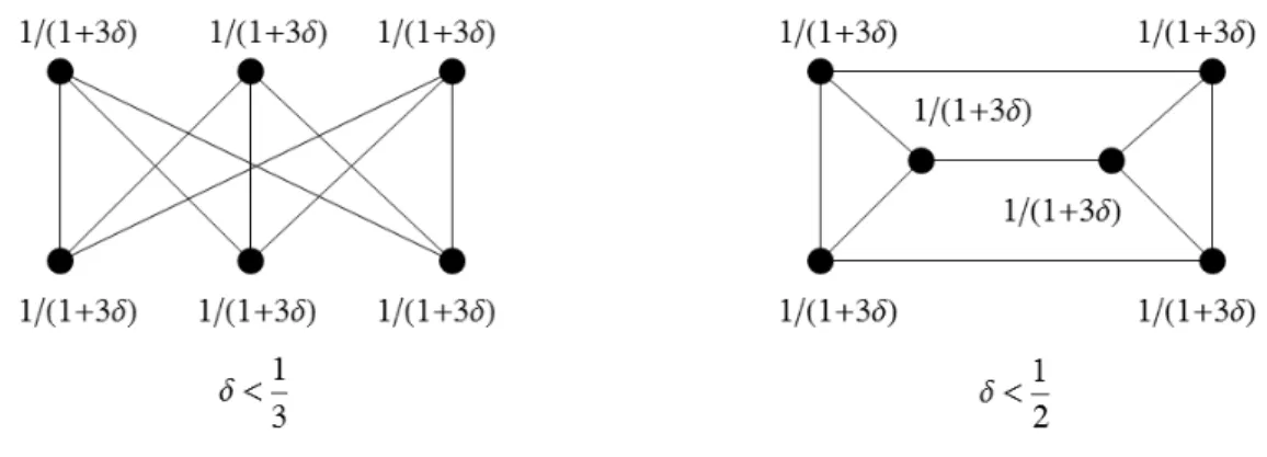
Example 4. Unique and Corner Equilibria. Consider the graph in Figure 4. min(G) = 1=3:
For < 1=3, there is a unique equilibrium, where each agent plays 1+31 . For 1=3 < 1 there
3 4When = 1=
min(G), the potential is concave but not strictly concave. While multiple equilibria may
emerge, the equilibrium set is strongly structured. Equilibria form a convex set, and all equilibria yield the same aggregate action. In addition, one equilibrium is the limit of the unique equilibrium for < 1= min(G)as tends
to 1= min(G)from below. 3 5
Figure 4: Lowest Eigenvalue and Unique and Corner Equilibria
are three equilibria: the interior equilibrium where each agent plays 1+ 31 , and two specialized equilibria where agents on one side play 1 and agents on the other side play 0. In this range, the interior equilibrium is a saddle point and the specialized equilibria are global maxima of the potential.
This example generalizes; Propositions 2 and 3 give tight conditions for particular graphs and for all regular graphs. When every agent has k neighbors, for any 2 [0; 1] it is an equilibrium for each agent to play xi = 1=(1 + k). If < 1= min(G), this is the unique equilibrium. If
> 1= min(G), an interior vector cannot maximize the potential. Hence there must be another
equilibrium, which is a corner.36
Corollary 1. For regular graphs, there is a unique equilibrium if and only if < 1= min(G)
and this equilibrium is interior. If 1= min(G) there are both interior and corner equilibria.
Combining Propositions 2, 3, and previous results, for a graph G we can divide the range of into four parts. In the lowest part, 0 < BCAZ there is a unique and interior equilibrium. The equilibrium vector is x = (I + G) 11= 1 c( ; G): In the lower-middle range,
BCAZ <
1= min(G), there is a unique equilibrium, which is either interior or corner. In the upper-middle
range, 1= min(G) < 1, multiple equilibria are possible, and a corner equilibrium always
exists. For active agents, in any equilibrium, xA = (I + GA) 11 = 1 c( ; GA): At = 1;
for any graph there is an equilibrium vector where xA = 1, and the active agents constitute a
maximal independent set of the graph. We see these ranges in Examples 1, 2, 3, and 4.
3 6At = 1=
IV. Stable Equilibria
In this section we delve more deeply into the problem of multiple equilibria and identify those equilibria which are stable. We show the lowest eigenvalue of a graph is key to stability, as it is key to unique equilibria.
A. Asymptotically Stable Equilibria
We consider a continuous adjustment process, asking when a Nash equilibrium x is an asymptot-ically stable stationary state (Weibull (1995)) of the following system of di¤erential equations:
x1 = h1(x) = f1(x; ; G) x1
.. .
xn = hn(x) = fn(x; ; G) xn
where fi(x; ; G) is agent i’s best response (2). In vector notation _x = H(x), where H =
(h1; : : : hn) : Rn! Rn. By construction, x is a stationary state of this system if and only if x is a
Nash equilibrium of our games.37 A Nash equilibrium x is asymptotically stable when this system of di¤erential equations converges back to x following any small enough perturbation.38
Next, say that a (local or global) maximum x of the potential is locally strict if there is an open neighborhood of x in Rn+ on which ' does not have any other maximum. We can then show
there is a one-to-one relationship between locally strict maxima and stable equilibria:
Lemma 2. An equilibrium x is asymptotically stable if and only if x is a locally strict maximum of the potential.
To prove this result note that the opposite of the potential function, ', provides a natural Lyapunov function for the system of di¤erential equations. In particular, the potential must
3 7
We also looked at discrete Nash tâtonnement, as in Bramoullé & Kranton (2007). We …nd equilibria stable to Nash tâtonnement are (almost always) asymptotically stable. But the reverse is not true, and Nash tâtonnement stable equilibria may fail to exist in large regions of the parameter space. (Proofs are available upon request.) In contrast, asymptotically stable equilibria exist generically, as shown below.
3 8
Following Weibull (1995, De…nition 6.5, p.243), we de…ne asymptotic stability as follows: Introduce B(x; ") = fy 2 Rn
+: jjy xjj < "g and (t; y) the value at time t of the unique solution to the system di¤erential equations
that starts at y. (So, (0; y) = y). By de…nition, x is Lyapunov stable if 8" > 0; 9 > 0 : 8y 2 B(x; ), 8t 0, (t; y) 2 B(x; "). Then, x is asymptotically stable if it is Lyapunov stable and if 9" > 0 : 8y 2 B(x; "),
always increase along the trajectories of the system: dtd'(x(t)) =Pi@x@'
i_xi= r'(x) H(x) > 0 if
x is not an equilibrium.
Thus, stability eliminates the Nash equilibria that are saddle points of the potential and maxima that are not locally strict. Observe that for any G and almost every , the number of equilibria is …nite and, hence, maxima of the potential are all locally strict. Since for any and G, the potential has a global maximum, a stable equilibrium exists for almost every .
B. Necessary and Su¢ cient Condition for Stablility
Here we …nd a necessary and su¢ cient condition for stable equilibria by looking at the shape of the potential at an equilibrium x. For unique equilibria, we looked at global concavity of the potential. Here we focus on the shape of the potential locally, in the neighborhood of an equilibrium x: We …nd that for an equilibrium x, with active agents A, min(GA) gives (almost
always) a necessary and su¢ cient condition for stability.
To make our argument, we establish that we need only look at active agents and the subgraph GA. For inactive agents, there are two types: (a) those for whom a small reduction in neighbors’
actions would not lead them to change their play; i.e., agents for whom Pjgijxj > 1; and (b)
those for whom a small reduction would lead them to increase their play; i.e., Pjgijxj = 1:
The …rst type can be safely ignored (see Appendix). The second type, which we call knife-edge agents must be examined, since even a small reduction in a neighbor’s action would lead them to increase their play. We show in the Appendix however, that for any graph G for almost every ; there are no knife-edge agents in any equilibrium. Thus, almost always, the relevant shape of the potential around an equilibrium x is determined only by GA. In particular, from GA we derive
the curvature of the potential on the subset of the action space restricted to active agents. Generically: When min(GA) is large relative to , the potential function is strictly concave
on the action space of active agents. The graph absorbs the impact of changes in play, and the equilibrium is stable. When min(GA) is small relative to , the potential function is not concave
on the action space of action agents. A small change reverberates through the network, and the equilibrium is not stable. This gives a generic necessary and su¢ cient condition for stability: an equilibrium is stable if and only if < 1= min(GA):39
3 9
Non-generically: In the presence of knife-edge agents, < 1= min(GA) is necessary for
stability. We derive the precise necessary and su¢ cient condition in this case in the Appendix. Summarizing:
Proposition 4. Consider a graph G and a Nash equilibrium x with active agents A. If there are no knife-edge agents, x is stable if and only if < 1= min(GA). If there are knife-edge agents,
if x is stable then < 1= min(GA).
C. Shape of Stable Equilibria
We can also determine the shape of stable equilibria. When < 1= min(G), by Proposition
2, there is a unique equilibrium. This equilibrium is interior or corner, and it is stable. When > 1= min(G); there can be multiple equilibria and by Proposition 3 at least one equilibrium
is a corner. Since for interior equilibria A = N , our stablility condition eliminates all the interior equilibria in this range,
Corollary 2. For a graph G, if > 1= min(G), all stable equilibria are corners.
The following examples illustrate the lowest eigenvalue stability condition and the shape of stable of equilibria.
Figure 5: Lowest Eigenvalue and Stable Equilibria
if A is such that GA is empty and there are no knife edge agents. A is then a maximal independent set, the
Example 5. Stable Equilibria and the Lowest Eigenvalue. Consider the graph on the left of Figure 5, which is complete bipartite, and the pro…le xi = 1+31 for all i which is a Nash
equilibrium for any 2 [0; 1]. For this graph, min(G) = 3, hence this equilibrum is stable
for < 1=3. For 1=3 < ; only corner equilibria are stable. Next consider the “prism” graph in Figure 5. Since it is also regular with k = 3, xi = 1+31 is a Nash equilibrium for any 2 [0; 1].
Here, min(G) = 2, and hence, the interior equilibrium is stable for < 1=2: For 1=2 < ; only
corner equilibria are stable. For intuition, compare what happens after perturbing one agent’s play in the bipartite graph to perturbing one agent’s play in the prism graph. Let some agent i play 1+31 + " In the bipartite graph, all three agents on the other side will adjust their play by the full amount: In the prism graph, two of the agents linked to i are also linked to each other and “share” the adjustment. Hence, the interior equilibrium is stable for a higher in the prism graph than in the complete bipartite graph.
Example 6. Stable Equilibria versus Nash Equilibria. The stability condition can elimi-nate many Nash equilibria in the range > 1= min(G). For example, in the complex network
pictured in Figure 3, at = 0:35 two among the three equilibria are stable. At = 0:55, only seven among the thirty-one equilibria are stable.
This analysis gives a general intution that stable equilibria involve smaller sets of active agents. Interior equilibria— where everyone takes positive action— are only stable when they are the unique equilibrium. Otherwise, only corner equilibria are stable. Furthermore, the sets of active agents of stable equilibria are minimal in terms of inclusion. Consider two equilibria x and x0 with active agents A and A0. If A A0, then stability of x implies instability of x0 (see Appendix). This is consistent with the fact that A A0 ) min(GA) min(GA0).40 Smaller
subgraphs have more absorptive capacity.
To summarize our stability results: For any graph G and almost every , a stable equilibrium exists. If < 1= min(G), the unique equilibrium is asymptotically stable; it is a corner or
an interior equilibrium. If > 1= min(G); the stable equilibria are corners. The stability
conditions focus our attention on particular equilibria with small sets of active agents, and Section VI conducts comparative statics on these equilibria.
4 0
This relationship follows from the interlacing eigenvalue theorem, e.g. Horn & Johnson (1985, p.185). Note that any perturbation on the smaller subgraph can be replicated on the larger one, but not vice versa.
V. Lowest Eigenvalue of a Graph
The previous sections show the lowest eigenvalue of a graph is critical to unique and stable equilibria. Here we how this graph statistic relates to network structure.
We can gain much intuition from looking at the two networks in Figure 5. For the complete bipartite graph min(G) = 3, and for the prism graph min(G) = 2. Each has nine links,
and each is a regular graph. But in the complete bipartite graph there are two distinct sets of agents, with links between the sets but not within each set. The complete bipartite graph has no triangles. In the prism graph, on the other hand, there are triangles— what sociologists call “triadic closures;” friends of an agent i are also friends with each other. Loosely speaking, the lowest eigenvalue involves a tradeo¤ between more links and more closure.
We can formalize this intuition as follows. Let G be the set of all possible graphs for n agents. Let G 2 G be a graph with the smallest lowest eigenvalue; i.e., min(G ) min(G) for all
G2 G.
First, G is a complete bipartite graph with as equal size sides as possible.41
Eigenvalue Result 1. G is a complete bipartite graph. For n even, k = n=2 for all agents. For n odd, n+12 agents have n 12 links, and n 12 agents have n+12 links.
Intuitively, the complete bipartite structure maximizes the ampli…cation of shocks. A change in play by any agent reverberates through the network. In contrast, a complete graph, where all agents are connected (so there is complete triadic closure), contains the shocks by any agent.42
Second, for any graph G 6= G we can cut and add links to G to yield a G0 that has a smaller lowest eigenvalue. We essentially make the graph “more bipartite.” For any G, there exists a partition of the population in two sets R and S such that adding links between or cutting links within the sets weakly reduces the lowest eigenvalue. We identify these sets from an eigenvector associated with min(G):43
Eigenvalue Result 2. Consider a graph G 6= G : Let u be an eigenvector for min(G), and let
R = fi : ui 0g and S = fi : ui < 0g. Form a new graph G0 by removing any number of links
(i; j) 2 R R or S S, and adding any number of links (k; l) 2 R S. Then min(G0) min(G)
4 1
We thank Noga Alon for his help and providing us a proof of this result. See also Constantine (1985).
4 2
Intuitively, by adding links between sets, agents’ actions directly impact more agents. Cutting links within sets reduces triadic closures, and agents’actions are less contained by the graph.
Third, a graph has the smallest lowest eigenvalue when it has as many links as possible with no triangles. More links increase the impact of shocks, but triadic closures contain them. We have:44
Eigenvalue Result 3. G is equivalent to the graph G 2 G with the greatest number of links and no triadic closure.
The problem of …nding the graph for n agents with the smallest lowest eigenvalue for a …xed number of links is much more di¢ cult and has only recently been addressed by mathematicians.45
-10 -8 -6 -4 -2 0 -18 -16 -14 -12
Circle with k nearest neighbors Poisson random graph
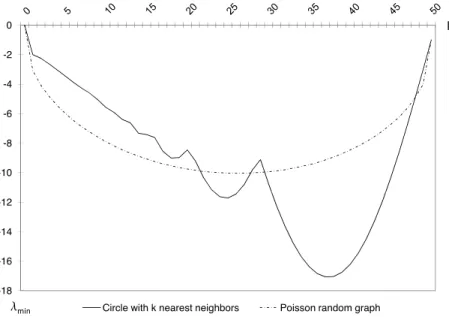
Figure 6: Lowest Eigenvalue and Network Links
For particular gaph families, we can compute lowest eigenvalues to see the tradeo¤s as links are added to a network. We depict in Figure 6 how the lowest eigenvalue varies with number of links for two well-known structures: Bernouilli random graphs and circles. In Bernouilli random graphs, the expected lowest eigenvalue is …rst decreasing and then increasing in the probability
4 4See Theorem 2, p.6, and Exercise 4, p.28, in Bollobas (1998). 4 5
of connection. Starting from the empty graph, most links are between sets of agents. The new links, however, eventually form more triangles (i.e., links within sets of agents), and the absorptive capacity of the network increases. This relationship is more irregular for the circle, despite the regularity of its structure. The lowest eigenvalue for the circle also reaches its minimum for a higher number of connections than the Bernoulli graph.46
VI. Comparing Equilibria
In this section we compare equilibrium outcomes in terms of aggregate play,Pni=1xi. We can use
the potential function to do so, since the potential evaluated at an equilibrium is always equal to one-half of total play; that is, for a given and G and an equilibrium x( ; G), '(x; ; G) =
1 2
Pn
i=1xi( ; G):47
A. Aggregate Play for a given and G
Equilibria with fewer active agents— in terms of set of inclusion— always have a higher level of aggregate action. That is, consider an equilibrium x with active agents A and equilibrium x0with
active agents A0, where A A0. Then, Pix0i Pixi. Concentrating actions on fewer agents
increases overall play. This …nding reinforces our intuition about small sets of active agents. Fewer active agents is related to both higher aggregate play and greater stability.
B. Comparative Statics— Aggregate Play for di¤erent and G
Next we conduct comparative statics on and G: Comparative statics are di¢ cult in games of strategic substitutes since direct and indirect e¤ects generally pull in opposite directions. Consider a change in a parameter that induces agent i to increase her action. In response, i’s neighbors decrease their actions, and their neighbors increase their actions, and so on. The resulting impact on play could be complicated and nonmonotonic. We use the potential function to overcome these di¢ culties, and we obtain clean local and global comparative static results.
4 6
We also studied small-world graphs. Consider the original Watts & Strogatz (1998) procedure: From a circle, rewire each link at random with probability p. As p varies from 0 to 1, the expected lowest eigenvalue varies smoothly and monotonically from the lowest eigenvalue of the circle to the expected lowest eigenvalue of the Bernouilli random graph.
4 7
Let x be an equilibrium with active agents A. Since xN A= o, xT(I+ G)x = xTA(I+ GA)xA. By Proposition
1, (I + GA)xA= 1. Since xTA1= xT1, '(x) = 12x T1.
B.1. Global Comparative Statics— Higher , More Links
Consider a and G and an equilibrium x ( ; G) which is a global maximum of '(x; ; G). This equilibrium has the highest aggregate play of all equilibria for and G. We show that any large or small increase in or any additional link to the graph always leads to an equilibrium with lower total play. Thus, while some agents may increase their actions, the decreases dominate.
Proposition 5. Consider a and G and an equilibrium x ( ; G): Consider a 0 and G0 where
0 and G is a subgraph of G0 and any equilibrium vector x( 0; G0). Then
n X i=1 xi( 0; G0) n X i=1 xi( ; G):
To understand this result, notice that for any vector x, '(x; 0; G0) '(x; ; G); that is, holding play …xed, the value of the potential is lower when the payo¤ impact is higher and/or more agents are connected. Therefore, we have
'(x( 0; G0); 0; G0) '(x ( 0; G0); 0; G0) '(x ( 0; G0); ; G) '(x ( ; G); ; G)
where the third inequality holds because x ( ; G) is a global maximum of the potential '(x; ; G).48 The decrease in aggregate actions is usually strict.49
Previous comparative statics results in the literature are special cases. For low , Theorem 2 in Ballester, Calvó-Armengol & Zenou (2006) says if G is a subgraph of G0, 0, and there is a unique interior equilibrium x for ( ; G) and x0 for ( 0; G0), then Pix0i Pixi. For = 1,
Bramoullé & Kranton’s (2007) example for the circle generalizes to the following: a specialized equilibrium with a largest maximal independent set of agents is always a global maximum of the potential and yields highest aggregate play (see Appendix). This …nding, along with Proposition 5, implies that the number of nodes in a largest maximal independent set decreases when more links are added to a graph. Galeotti, Goyal, Jackson, Vega-Redondo and Yariv (2006) noted this fact.
4 8
In contrast, we can build examples where the lowest total e¤ort in equilibrium is non-monotonic in or G.
4 9
See the Appendix. Precisely, suppose that < 0 and G = G0. Then, aggregate actions decrease strictly when no global maximum on and G is specialized. In contrast, if G G0and is unchanged, aggregate e¤ort decreases
B.2. Local Comparative Statics— Higher , More Links, Same Support
We now consider local changes. We start with a stable equilibrium. We then increase the payo¤ impact or add a link to the graph and look at equilibria that have the same or smaller set of active agents as the initial equilibrium. We again …nd that aggregate actions decrease.
Proposition 6. For and G, consider a stable equilibrium x( ; G) with active agents A. Now consider for 0 and G0 where 0 and G is a subgraph of G0 and consider any equilibrium x( 0; G0) with active agents A0 such that A0 A: Then, Pni=1x0i Pni=1xi.
Thus, we can compare a wide set of equilibria and …nd that total play drops when is higher or G has more links. The conditions of Proposition 6 hold when the new parameter values are “close enough” so that no new agents are active. The existence of such a close-by equilibrium when G = G0, for example, is guaranteed for almost any if the increase in is small.50
Comparative statics of individual actions, on the other hand, are generally non-monotonic. We show the direct and indirect e¤ects of a change in one player’s action are perfectly aligned if and only if G is bipartite (see Appendix). This result comes from the classic property that a graph is bipartite if and only if it has no odd cycles. On bipartite graphs, a positive shock on i’s action eventually leads to a decrease in the actions of every agent on the other side and to an increase in the actions of every agent on his side. In contrast, if G is not bipartite some direct and indirect e¤ects must go in opposite directions.
VII. Many More Games
Our analysis generalizes and applies to many more games. Recall in our basic model that gij =
gji 2 f0; 1g and xi = x for all i. The payo¤ impact parameter is a positive constant 2 [0; 1],
which combined with gij > 0 for all ij gives strategic substitutes. We show …rst how our results
directly extend to a strategic substitutes game with weighted graphs gij = gji 2 [0; 1] and
heterogeneous autarkic play.
We then consider three substantively di¤erent settings. In the …rst, agents have idiosyncratic payo¤ impact parameters i: One example is games where agents care about the average of others’
5 0
For almost any ; if A is the active set of agents for an equilibrium for and G there exists " > 0 such that if j 0 j ", A is also the active set of agents in an equilibrium for 0 and G.
play, which are ubiquitous in economics. With quadratic payo¤s, best replies are linear, and the impact parameters are heterogeneous and depend on an agent’s position in the graph. Second, we consider strategic substitutes and complements. Pure complements have been analyzed in previous literature; the analysis is relatively straightforward, and our tools easily apply. For the more complicated general setting with any mix of substitutes or complements, we show how results extend. Finally, we discuss games with non-linear best replies.
Heterogeneous autarkic play and weighted graphs. Consider the model in the text with heterogeneous autarkic play xi and a weighted graph gij = gji2 [0; 1]. The best-reply is now
fi(x) = max 0 @0; xi n X j=1 gijxj 1 A
where xi > 0 8i and 2 [0; 1]. Let x (x1; : : : xn). This model captures at least two
well-known games, written in a network form: (a) a linear-demand Cournot model with di¤erentiated products where …rms have di¤erent marginal costs, and (b) strategic private provision of public goods à la Bergstrom, Blume & Varian (1986) where consumers have di¤erent incomes.51
Our equilibrium analysis directly extends. The Nash conditions in Proposition 1 hold. The potential here is '(x) = xTx 1
2xT(I + G)x. Since the Hessian, r
2'; is not a¤ected by x,
all the results for unique and stable equilibria— Propositions 2, 3, and 4— apply as in the basic model.
Only the comparative statics results have to be modi…ed. Now for an equilibrium x; '(x) =
1 2
Pn
i=1xixi. We weigh individual actions by their thresholds and compare divergences from
autarkic play. E.g., for a given and G and a global maximum equilibrium x ( ; G), there is a decrease in weighted total actions for 0 and G a subgraph of G0; i.e., Pn
i=1xixi( 0; G0)
Pn
i=1xixi( ; G). Furthermore, we have clean comparative statics with respect to x; the weighted
sum of actions increases weakly when individual thresholds increase.
Heterogenous payo¤ impacts and “linear-in-means” games. We now study games where
5 1To see this, let each individual have Cobb-Douglas utility and allocate income, w
i, between private good
consumption, qi, and public good provision, xi. Let p the relative price of the public good. Bene…ts from the
public good are ‡ow to neighbors, weighted by 2 [0; 1]. Individual i then maximizes Ui= qi(xi+ Pigijxj)1
subject to the budget constraint qi+ pxi wi. Simple computations yield the correspondence with xi= 1p wi
and = . Note that even if = 1, < 1. When own and neighbors’ contributions are perfect substitutes in payo¤s Ui, they are imperfect substitutes in the best reply function.
the impact of others’play, captured in , can vary across agents. Thus far, we have considered games where a agent i’s best response is linear in the weighted sum of his neighbors’ play,
P
jgijxj. In many economic applications, the parameter may not be the same across all
agents and may depend on an agent’s graph position. For each agent i, we have i(G) and i’s
linear best reply involves i(G) Pjgijxj: We can use our techniques to study any such game.
Consider, for example, settings where agents care about the average play of other play-ers. Many games in microeconomics and macroeconomics— coordination games/beauty con-tests/social interactions games/investment games— have this feature. In many models, agents also have quadratic payo¤s.52 While in some settings agents desire to coordinate their actions, other settings involve strategic substitutes, as when agents want to invest in di¤erent technolo-gies. The standard treatments do not include networks, but a network treatment could transform the analysis. It would allow for social, geographic, and information structures and for mixes of strategic substitutes and complements. We call such models linear-in-means games. For each agent i, i(G) = k1i, where is a constant and recall ki is the number of i’s neighbors, and i’s
best reply is fi(x) = max 0 @0; 1 1 ki 0 @ n X j=1 gijxj 1 A 1 A ;
with 2 [0; 1]; gij = gji 2 f0; 1g, and 8i; ki6= 0. When G is not regular so that agents may have
di¤erent numbers of neighbors, k1
igij 6=
1
kjgji, and the game with (modi…ed) quadratic payo¤s ~Ui
does not have a potential. But by appropriate rescaling of the payo¤s, we obtain a “weighted potential,” in the terminology of Monderer & Shapley (1996). De…ne ei = kiU~i. The game with
payo¤s ei has the same best-replies and equilibria as the game with payo¤s ~Ui. And we can
easily see that@2eii(x)
@xi@xj =
@2e i(x)
@xj@xi for all i 6= j. So this modi…ed game has a potential function:
'(x) =Pi(kixi 21kix2i) 12
P
jgijxixj.
We derive conditions for unique and stable equilibria as follows: Introduce the network ~Gsuch that ~gij = pkgij
ipkj. The potential is then strictly concave if and only if < 1= min( ~G). The
uniqueness condition now includes the absorptive capacity of the original graph “normalized”by agents’ degrees. Similarly, the potential is not concave if and only if > 1= min( ~G), and the
results on multiple and corner equilibria apply. The stability results in Section IV all hold, again
5 2
using ~G:
As for comparative statics, observe that if x is an equilibrium, '(x) =12Pikixi. Thus,
com-paring across global maxima, if increases, the sum of individual actions weighted by degrees decreases weakly.53 In contrast, the e¤ect of adding links to the original graph G is not imme-diate. Connecting two agents increases their degrees which changes the weights used to compute the aggregate index. We show in Appendix that this new positive e¤ect dominates the negative ones.
The rescaling procedure we describe works for any graph gij = gji 2 R and payo¤ impacts i(G) and it further indicates a class of directed graphs (gij 6= gji) where our results apply.
Consider a directed graph H and payo¤ impacts i such that for each i and j there are scalars
i and j with the property ihij = jhji.54 We can de…ne a graph H0 where for all i and j,
h0ij ihij = jhji h0ji. The analysis of a linear-best response game with graph H is then
equivalent to that of a symmetric graph H0 and idiosyncratic payo¤ impacts i = i= i.
Strategic substitutes and complements. First, consider the basic model except gij 2 [ 1; 0]
so that we have a game of pure strategic complements.55 The analysis of such games is relatively simple, as noted in Corbo et al. (2007). If < 1= max( G) there is a unique interior equilibrium.
With xi2 [0; 1), an equilibrium fails to exist if > 1= max( G) since complementarities have an
explosive e¤ect on actions. Since max( G) = min(G); this result matches Proposition 2. Our
results also show this unique, interior equilibrium (when it exists) is stable. Comparative statics are also straightforward. Following an increase in one agent i’s action, i’s neighbors increase their actions, then their neighbors increase theirs, and so on. Our analysis thus con…rms what we already know, via a di¤erent route.56 However, these clear-cut results break down as soon as any substituability is present.
The question then is how to approach a game that is any mix of strategic substitutes and
5 3The similarity with the model with heterogeneous thresholds is not a coincidence. Apply the change of variables
yi= xi=pki. Then ei= (ki)3=2yi 21yi2 Pjg~ijyiyj. This corresponds to a model with thresholds yi= (ki) 3=2
. Then,Piyiyi=Pikixi. These thresholds, however, are determined by the network.
5 4
This property holds if and only if in H, for every triangle i; j; k; hij hjk hki = hik hkj hji; that is, for a
triangle the product of bilateral links is the same clockwise and counterclockwise.
5 5
There are strategic complementarities when for all ij : gij 0and 0, or gij and 0: 5 6The potential is strictly concave if and only if < 1=
max( G). Proposition 2 shows that uniqueness holds in
that range. Because of the change of sign, Proposition 5 now says that aggregate action increases as complemen-tarities increase.
strategic complements; i.e., gij = gji 2 R. Because of complementarities, existence of a Nash
equilibrium is not always guaranteed when xi 2 [0; 1). One fruitful approach is to bound the
action space. With xi 2 [0; l], we have best-reply
fi(x) = min 0 @l; max 0 @0; 1 n X j=1 gijxj 1 A 1 A :
An equilibrium exists for any and G, and the potential and its properties are unchanged. However, we have new constraints on the problem (P). Our uniqueness and stability results then apply with appropriate reformulation of boundary conditions.
Non-Linear Best Replies. Our analysis can be applied, locally, to any continuous potential game (see Appendix). Consider a game with xi 2 R+ and payo¤ function Vi.57 Construct a
game e[x] where the payo¤s are given by the second-order Taylor approximations of the payo¤s Vi around x. Then, best-replies of e[x] are linear and approximate ’s best-replies around x;
they capture the precise shape of strategic interactions around x. Thus, x is a Nash equilibrium of if and only if it is a Nash equilibrium of e[x]. Furthermore, e[x] is a potential game when is a potential game, in which case it can be analyzed using our techniques and results. The study of e[x] may then provide relevant information for the study of . In particular, because the Hessians of the potentials are the same, when x is stable in e[x] it is stable in and the stability properties are usually equivalent. Future research, discussed next, will explore further such relationships.
VIII. Conclusion: Future Research
This paper brings a general network analysis to a wide class of games. A graph, or interaction matrix, gives whose actions directly a¤ect whom. This matrix can represent, variously, social links, geography or market structure. We unify two strands of previous work and study games that have the same linear best replies. A canonical game in this class is one with quadaratic payo¤s. Since all games in the class have the same best replies, they have the same equilibria. We derive equilibrium conditions for any graph and any level of payo¤ impact, using the theory
5 7