Publisher: Taylor & Francis & IAHS
Journal: Hydrological Sciences Journal
DOI: 10.1080/02626667.yyyy.nnnnnn
A comparative study for water temperature modelling in a small basin, the
Fourchue River, Quebec, Canada
Jaewon Kwak
1, Andre, St-Hilaire
2and Fetah Chebana
21Nakdong River Flood Control Office, Busan, South Korea,
2INRS-ETE, INRS, Quebec, Canada,
Corresponding author : A. St-Hilaire: email: [email protected]
Abstract
Analysis and forecasting of water temperature are important for water-ecological
management. The objective of this study is to compare models for water temperature during the
summer season for an impounded river. In a case study, we consider hydro-climatic and water
temperature data of the Fourchue River (St-Alexandre-de-Kamouraska, Quebec, Canada) from between 2011 to and 2014. Three different models were applied, which are broadly characterized as deterministic (CEQUEAU), stochastic (Auto-regressive Moving Average with eXogenous variables or
ARMAX) and nonlinear (Nonlinear Autoregressive with eXogenous variables or NARX). The
efficiency of each model was analyzed and compared. The rResults show that the ARMAX is the best performing water temperature model for the Fourchue River and the CEQUEAU model also
simulated water temperature adequately without the overfitting issues that seem to plague the
autoregressive models.
Keywords water temperature; CEQUEAU; ARMAX; NARX
1.
INTRODUCTION
Water temperature affects physical and biological processes in the river system and is one of
the most important physical characteristics for aquatic organisms (Beschta et al., 1987,; Hammitt and Cole, 1998,; Coutant, 1999,; Nunn et al., 2003). Among them, fish species are sensitive to water temperature for growth rate and spawning (Ojanguren et al., 2001; Selong et al., 2001; Lessard and
Comment [F1]: Check!
Comment [F2]: Remove commas in references and replace ; with ,
Hayes, 2003; Handeland et al., 2008). Furthermore, it is also an important factor for water quality
(Singh et al., 2004; Morrill et al., 2005; Chang, 2008). There are many models and studies which
contribute to more accurate water temperature simulations and forecasts. Caissie (2006) suggested
that most models can be classified into three categories: regression-based, deterministic and stochastic.
Following the early work of Johnson (1971) and Kothandaraman (1972), parametric statistical models
such as regressions have been applied in many studies (Benyahya et al., 2007a). Simple linear
regressions have been used with air temperature as a predictor (Crisp and Howson, 1982; Mackey and
Berrie, 1991; Stefan and Preud'Homme. 1993). Also, multiple regression (Jeppesen and Iversen, 1987;
Jourdonnais et al., 1992), logistic regression (Mohseni et al., 1998; Mohseni and Stefan, 1999), ridge
regression (Ahmadi‐Nedushan et al, 2007) and Gaussian-process regression (Grbi• et al, 2013) have been used in water temperature models.
Deterministic models are based on the governing laws of heat exchanges and they consider
the different energy fluxes and (in some cases) mixing process in the rivers with various degrees of
complexity (Morse, 1970; Caissie, 2006, 2007). Due to this, they are widely used in applications with
complex thermal in/outflows (Sinokrot and Stefan, 1993; Kim and Chapra, 1997; Younus et al., 2000;
Danner et al., 2012). However, these models typically require more data than statistical models
(Benyahya et al., 2007b). In contrast, stochastic models often require one or few predictors that are
correlated with water temperature (Caissie, 1998; Webb et al., 2008). This category of models is very
efficient when air temperatures are the only available data (Caissie, 2006). Hence, they have been
widely applied to estimate weekly/monthly water temperature (Mohseni et al., 1998; Benyahya et al.,
2007b, 2008), daily water temperature (Caissie et al., 1998, 2001; Pal’shin and Efremova, 2005;
Ahmadi‐Nedushan et al, 2007; Larnier et al., 2010) and hourly temperature (Mestekemper et al., 2010; Pike et al., 2013; Jeong et al., 2013). Furthermore, Artificial neural networks (ANN), which belong to
the non-parametric category (Chenard and Caissie, 2008; Sahoo et al., 2009; DeWeber and Wagner, 2013; Hadzima-Nyarko et al., 2014), k-nearest neighbors algorithm (k-NN), which is a nonlinear
dynamic model (Benyahya et al., 2008; Nowak et al., 2010; St‐Hilaire et al., 2012; Caldwell et al., 2013) and dynamic chaotic models (Sahoo et al., 2009) have been applied to estimate water
temperature. While the literature on water temperature modelling is growing rapidly, relatively few
comparative modelling studies have been completed on rivers with dams, especially in Canada.
The objective of this study is therefore to investigate the simulation efficiency of a number of
water temperature models using hydro-climatic variables in the context of regulated flows. The
models were compared on the Fourchue River basin, a forested catchment on which there is a
managed reservoir. The Fourchue River has been previously studied by Beaupré (2014). She
compared a deterministic model (SNTEMP; Bartholow, 1995) and a geostatistical model (Guillemette
et al., 2009) both upstream and downstream of the dam. Beaupré (2014) showed that the geostatistical
model outperformed SNTEMP for directly predicting temperature metrics that are relevant for
salmonids, especially when these metrics are calculated using simulated maximum temperatures. For
this follow-up study, hydro-climatic data were collected from 2011 to 2014 and models that represent
three categories: deterministic, stochastic and nonlinear were used.
2.
STUDY AREA AND DATA
The Fourchue River, with a drainage basin of 261 km2, is a tributary of the Du-Loup River, located in the eastern Quebec region, Canada. The Fourchue River is regulated by the Morin Dam,
with flows of between 0.06 to and 4.0 m3/, which discharged from the epilimnion zone of the reservoir (184 E.L.m to 188 E.L.m).
Fig. 1 Study area and measuring station.
Many factors influence water temperature variability, which can be classified into four
groups; atmospheric, topographic, hydrologic and streambed conditions. Selected predictors included
atmospheric variables because atmospheric conditions are mainly responsible for the heat exchange
processes. In addition, stream discharge was selected because it influences the heating capacity by
determining the volume of water in the river reach (Caissie, 2006), but also because all models
compared in this study need to be able to account for the impact of impoundment and the associated
regulated flows.
Formatted: Highlight Formatted: Highlight Formatted: Highlight Comment [F3]: Please replace equations with text
Formatted: Highlight
Comment [F4]: This unit should be more clearly defined
Formatted: Highlight
Comment [F5]: station or stations? Comment [F6]: Make sure all figures are cited in the text (Fig. 1 is not cited) – for example, Fig. 1, Fig. 2(a), Figs 3–4, Fig. 5(a)–(c). but Figure, in full, at the start of a sentence. Figure captions should be listed at the end, after the references and Tables
Atmospheric variables used as potential predictors include air temperature, solar radiation,
relative humidity and wind speed, which are known to be related to water temperature. Water
temperature were obtained during the summer seasons (June to September) from 2011 to 2014 with
Hobo Pro V2 thermographs (± 0.2° ℃C) sampling at 15- minutes intervals, and hourly solar
radiation data were measured with a Kipp and Zonen pyranometer (SP-LITE, ± 10uV/W/m2), connected to a Campbell Scientific CR1000 datalogger, powered by a solar panel and a 12- V battery. The water temperature loggers were deployed over a 8- km river reach, from directly downstream of the Morin Ddam to its confluence with the Du-Loup River. Air temperature and relative humidity were obtained from the Fourchue River meteorological station (Environment Canada;
http://climate.weather.gc.ca). Also, hydro-physiographic properties of the Fourchue River basin,
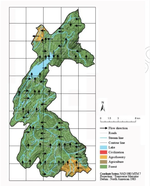
required to run the deterministic model, were extracted from a 3 km x× 3 km grid DEM and lLand-use map (http://srtm.csi.cgiar.org/) (Fig.ure 2).
Fig. 2 Hydro-physiographical characteristics of
the
study area
., showing
Map shows
land use,
whole squares (elementary hydrological units) and arrows indicat
eing
water routing used for
the deterministic (CEQUEAU) model.
3.
METHODOLOGY
3.1 Test statistics for selection of model and predictors selection
Given the plethora of potential models, five test statistics were used to identify the main
characteristics of collected temperature data and potential predictors in order to select reasonable
candidate models to simulate water temperatures of the Fourchue River. The considered tests are: the Spearman rank correlation coefficient for randomness (Myers and Well, 2003), the Ljung-Box Q test for autocorrelation (Ljung, 1978), Levene’s test for heteroscedasticity (Levene, 1960), the Lyapunov exponent test (Bask and Gençay, 1998) and the BDS statistics test for chaotic characteristic (Brock et
al. 1987) of data time series.
Mutual Information (I) was also used to select appropriate predictors among the collected
data set.,where I(X:Y) is a measure of the amount of information that one continuous random variable
X contains about another continuous random variable Y (Cover and Thomas, 2006):
I(X: Y) = ∫ ∫ 𝑝(𝑥, 𝑦) log �𝑌 𝑋 𝑝(𝑥) 𝑝(𝑦)𝑝(𝑥,𝑦) � 𝑑𝑥 𝑑𝑦 (1)
where, 𝑝(𝑥) and 𝑝(𝑦) are the marginal probability density functions of X and Y and 𝑝(𝑥, 𝑦) is the joint probability density function. The mutual information will be larger for variables which have a stronger relation and vice versa. So, predictors selection based on value of I(X:Y) of
each input variable with the output variable can be used to identify the most important predictors
(Battiti, 1994).
3.2 Water tTemperature mModels
Given the large number of available water temperature models in use, the aforementioned
criteria were used to find the most suitable ones for the Fourchue River. Three types of candidate
models were considered: (ai) one a deterministic model called CEQUEAU (Morin et al., 1998); (bii) the ARMAX (AautoRregressive-Mmoving Aaverage with eXxogenous terms) model, which is in the stochastic category; and (ciii) the NARX (Nonlinear AutoRegressive model with eXogeneous input) for the nonlinear approach.
The CEQUEAU model is a hydrological model that is combined with a heat budget model and has shown applicability in Canada (Morin and Slivitzky, 1992; St-Hilaire et al., 2000, 2003;
Seiller and Anctil, 2014) and in other countries (Dibike and Coulibaly, 2005; Ba et al., 2009; Sauquet
et al., 2009; Eleuch et al., 2010). The ARMAX model is useful when the data are noisy, so it has the potential to show good results and provide flexibility in describing the properties of the noise
associated with water temperature time series (Breaker and Brewster, 2009) and NARX models also
show good performance for several types of chaotic time series (Diaconescu, 2008).
Formatted: Font: Italic Formatted: Font: Italic Formatted: Font: Italic Formatted: Font: Italic Comment [F7]: Make variables italic, ‘d’ not italic; use of Equation Editor 3.0 or MathType is preferred so that equation fonts are the same as the text. Also use text and symbols where possible in the text below, rather than equation terms. Make variables consistent between text and equations, i.e. in terms of italics
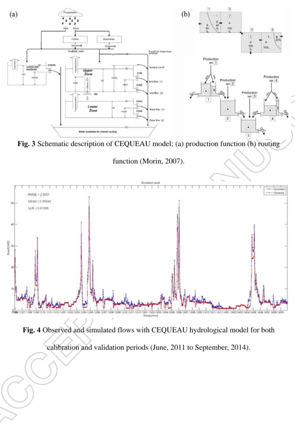
3.2.1 CEQUEAU model: deterministic approach
The CEQUEAU model is a semi-distributed hydrologic model which takes into account the
hydro-physiographic characteristics of the basin (Morin et al., 1981). It is based on a water balance calculations and subsequent runoff generation through a set of elementary hydrological units called
“whole squares”, which are further divided in “partial squares” according to the water divide (Morin
et al., 1998). The CEQUEAU model comprises two functions to describe the runoff mechanism and
upstream-downstream routing: (a) the production function represents vertical water routing from
rainfall, snowmelt, infiltration and evapotranspiration used in water-balance calculations; and (b) the routing function is used to estimate the amount of water transiting to the downstream partial squares
and ultimately to the outlet of the basin in the drainage network (Figure 3).
Fig. 3 Schematic description of CEQUEAU model
:;
(a) production function (b) routing
function (Morin, 2007).
Prior to modelling water temperature, the hydrological model component of CEQEAU needs
to be calibrated against observed flows and/or water levels. Model parameters were adjusted by hand
using water level and runoff data of the Morin Dam between June 2011 and September 2014 (Figure
4). Subsequently, the water temperature module of the CEQEAU model was used (Morin et al, 1998).
This component computes a heat budget on each elementary hydrological unit (whole squares) based
on the volume of water modelled by the hydrological module of CEQUEAU. Heat budget terms
include incoming short wave solar radiation, net longwave radiation, latent heat, sensible heat, heat
advected from upstream, heat loss downstream and local contributions from groundwater and
interflow. Each heat budget term can be adjusted using a weighing coefficient. Average water
temperatures are thus estimated at a daily time step.
Fig. 4 Observed and simulated flows with CEQUEAU hydrological model for both
Comment [F8]: No italics needed
calibration and validation periods (June
,
2011 to September
,
2014).
3.2.2 ARMAX: stochastic approach
The ARMAX model is useful when the input data have noise, has more flexibility than other
stochastic model, such as ARMA or ARX, and is defined as:
A(𝑧)𝑦(𝑡) = 𝐵(𝑧)𝑢(𝑡 − 𝑘) + 𝐶(𝑧)𝑒(𝑡) (2)
wWhere 𝑦(𝑡) is the output, 𝑢(𝑡) is the input, 𝑒(𝑡) is the system error and 𝑘 is the time delay of the system. The terms A(z), B(z), and C(z) are polynomial with respect to the backward shift operator 𝑧−1 and defined as:
A(𝑧) = 1 + 𝑎1𝑧−1+ ⋯ + 𝑎𝑡𝑎𝑧−𝑡𝑎 B(z) = 𝑏0+ 𝑏1𝑧−1+ ⋯ + 𝑏𝑡𝑏𝑧−(𝑡𝑏−1)
𝐶(𝑧) = 1 + 𝑐1𝑧−1+ ⋯ + 𝑐𝑡𝑐𝑧−𝑡𝑐 (3)
In this study, the ARMAX model has second order AR and MA processes and one day time
lag (𝑘), which were optimized by trial and error method (ARMAX(2,2,1)).
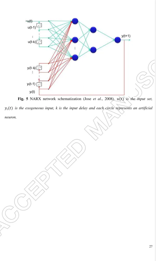
3.2.3 NARX : nonlinear approach
Non-linear AutoRegressive model with eXogeneous input (NARX), is a special form of
recurrent neural network with the outputs fed back to the input by delay line (Haykin, 1999). It has
been demonstrated that they are well suited for modeling nonlinear and chaotic time series (Lin et al,
1996; Gao and Joo, 2005) and also solve vanishing gradient problem, which occur in the prediction of
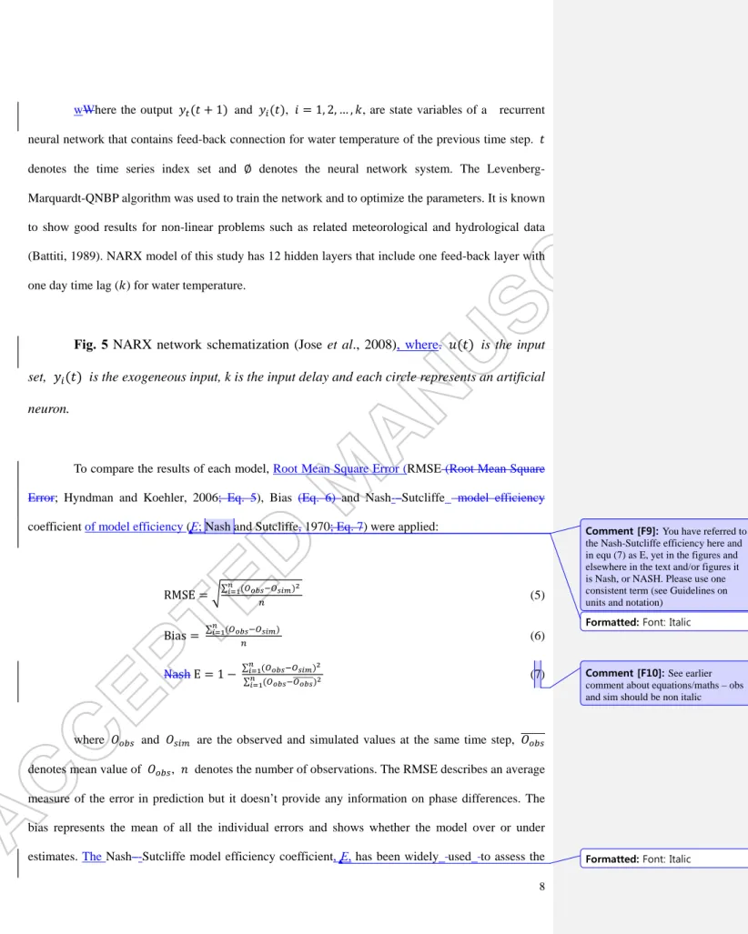
nonlinear data (Haykin, 1999). A NARX model can be expressed as (Eq(4) and Figure 5):
𝑦𝑡(𝑡 + 1) = �∅(𝑢𝑦 (𝑡), 𝑦𝑖(𝑡), 𝑖 = 1
𝑖(𝑡), 𝑖 = 2,3, … , 𝑘� (4)
wWhere the output 𝑦𝑡(𝑡 + 1) and 𝑦𝑖(𝑡), 𝑖 = 1, 2, … , 𝑘, are state variables of a recurrent neural network that contains feed-back connection for water temperature of the previous time step. 𝑡 denotes the time series index set and ∅ denotes the neural network system. The Levenberg-Marquardt-QNBP algorithm was used to train the network and to optimize the parameters. It is known
to show good results for non-linear problems such as related meteorological and hydrological data
(Battiti, 1989). NARX model of this study has 12 hidden layers that include one feed-back layer with
one day time lag (𝑘) for water temperature.
Fig. 5 NARX network schematization (Jose et al., 2008)
, where.
𝑢(𝑡) is the input
set,
𝑦
𝑖(𝑡) is the exogeneous input, k is the input delay and each circle represents an artificial
neuron.
To compare the results of each model, Root Mean Square Error (RMSE (Root Mean Square Error; Hyndman and Koehler, 2006; Eq. 5), Bias (Eq. 6) and Nash-–Sutcliffe model efficiency coefficient of model efficiency (E; Nash and Sutcliffe, 1970; Eq. 7) were applied:
RMSE = �∑𝑛𝑠=1(𝑂𝑜𝑏𝑜−𝑂𝑜𝑠𝑠)2 𝑛 (5) Bias = ∑𝑛𝑠=1(𝑂𝑜𝑏𝑜−𝑂𝑜𝑠𝑠) 𝑛 (6) Nash E = 1 − ∑𝑛𝑠=1(𝑂𝑜𝑏𝑜−𝑂𝑜𝑠𝑠)2 ∑𝑛𝑠=1(𝑂𝑜𝑏𝑜−𝑂�������)𝑜𝑏𝑜2 (7)
where 𝑂𝑜𝑜𝑜 and 𝑂𝑜𝑖𝑠 are the observed and simulated values at the same time step, 𝑂������ 𝑜𝑜𝑜 denotes mean value of 𝑂𝑜𝑜𝑜, 𝑛 denotes the number of observations. The RMSE describes an average measure of the error in prediction but it doesn’t provide any information on phase differences. The
bias represents the mean of all the individual errors and shows whether the model over or under
estimates. The Nash–-Sutcliffe model efficiency coefficient, E, has been widely used to assess the
Formatted: Font: Italic
Comment [F9]: You have referred to the Nash-Sutcliffe efficiency here and in equ (7) as E, yet in the figures and elsewhere in the text and/or figures it is Nash, or NASH. Please use one consistent term (see Guidelines on units and notation)
Comment [F10]: See earlier comment about equations/maths – obs and sim should be non italic
Formatted: Font: Italic
predictive power of hydrological models (Moriasi et al., 2007).
4.
MODEL AND PREDICTOR SELECTION
We applied five test statistics (Spearman rank correlation coefficient, Ljung-Box Q, Levene,
Lyapunov exponent and BDS test) to determine the characteristics of the collected data (water and air
temperature, runoff, solar radiation, relative humidity and wind speed). Through the Spearman Rank
Correlation and Ljung-Box Q tests, all time series except solar radiation, which is a truly random
series (calculated 0.154 versus critical value 1.96 in the Spearman Rank Corr. Coeff. test, and p-value
0.997 in Ljung Box-Q test), were identified as stochastic time series. Other test results are shown in
Table 1.
Table 1 Test statistics for each dependent and independent variables.
As the result of test statistics indicate, solar radiation data are categorized as a random series,
runoff is a chaotic time series which has heteroskedasticity, relative humidity is also a chaotic time
series and other data time series (water temperature, air temperature and wind speed) are categorized
as nonlinear stochastic time series. Water temperature (target variable) can be classified as a nonlinear
stochastic time series and most of the input predictors are chaotic, nonlinear and stochastic time series.
Therefore, models such as multiple regression or zero-mean AR(1) models that cannot account for
such characteristics are not eligible to simulate water temperatures in the Fourchue River. From the
conclusions drawn from Table 1, the NARX and ARMAX models were selected because they are
adapted to model time series such as water temperature and they show good results with chaotic and
nonlinear data (Diaconescu, 2008; Diversi et al., 2011). These models will be compared to the
deterministic model (CEQUEAU).
Also, selection of the appropriate inputs is one of the main challenges. For the stochastic
models, this selection can be done by trial and error models with different number of input variables
(Grbi• et al., 2013). However, that trial and error method can be time-consuming and lead to poor
Formatted: Font: Italic
Comment [F11]: p value [hyphen not needed]
performance for neural networks (Haykin, 1999; Maier and Dandy, 2000). So, mutual information
theory was employed to select the most important predictor variables for the NARX models. As the
result of the computation of mutual information, air temperature (1.28), runoff (0.82) and relative
humidity (1.09) are shown to have more meaningful mutual information value with water temperature
than solar radiation (0.30) and wind speed (0.09). The positive high value of the mutual information is
indicative that the potential predictor has a stronger relation with the dependent variable, i.e. water
temperature (May et al., 2008; Sahoo et al., 2009). So, air temperature, runoff and relative humidity
were selected as the appropriate predictors.
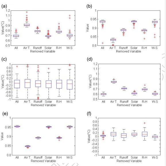
To corroborate the results of the Mutual Information analysis, a trial and error jackknife
method was used. One of the hydro-climatic variable was removed from the input data set, which
consist of air temperature, runoff, relative humidity, solar radiation and wind speed. Then the NARX
and ARMAX models were simulated 200 times with each removed data set. Figure 6 shows boxplots
of the evaluation result of simulation with each removed set.
Fig. 6 Performance statistics from jackknife simulations to select predictor
:;
(a)
RMSE of NARX, (b)
ENash
of NARX, (c) Bias of NARX, (d) RMSE of ARMAX, (e)
Nash
E
of ARMAX,
and
(f) Bias of ARMAX.
As the mutual information results and boxplots show and as expected, air temperature is the
most suitable predictor for water temperature simulation. Runoff and relative humidity are also
revealed as suitable independent predictors. The fact that runoff was included in the list of predictors
is of the utmost importance, given that the river is regulated and that the models must be able to
account for flow management. On the contrary, the inclusion of solar radiation and wind speed
showed no improvement and in some cases, slightly better results were obtained if they were removed
from the input data set.
Also, as shown in Ffig.ure 4, the summer season (June. to –September.) of 2011 has a high
runoff event (peaking at over 30 m3/s), while the other periods do not include such extreme events (i.e.
Formatted: Font: Italic Formatted: Font: Italic
flows remain below 10 m3/s). In spite of the inclusion of flow as a predictor, model performances are not as good during high runoff period as for the rest of the time. Longer time series will be required to
improve model calibration on the Fourchue River.
5.
RESULTS AND DISCUSSION
To partially overcome the challenges associated with the relatively small time series that can
be used form model calibration, we divided the data set in two cases and perform calibration and
validation in both cases.
Case 1: 2011, 2012, 2013 as calibration period and 2014 as validation period.
Case 2: 2012, 2013, 2014 as calibration period and 2011 as validation period.
The calibration results with selected models and predictors, which consist of air temperature,
runoff and relative humidity, are shown in Ffigures 7 and 8.
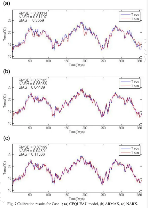
Fig. 7 Calibration results for Case 1
:;
(a) CEQUEAU model, (b) ARMAX, (c) NARX.
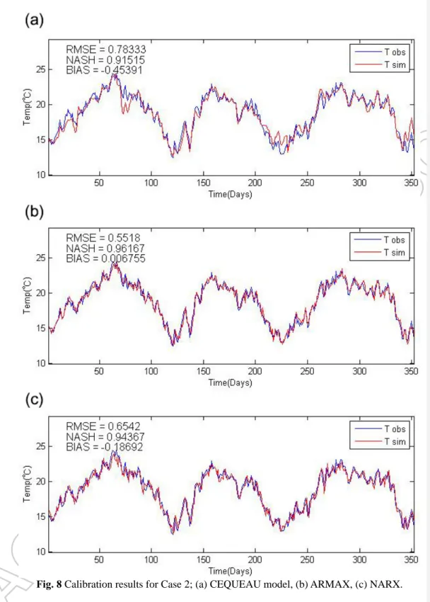
Fig. 8 Calibration results for Case 2
:;
(a) CEQUEAU model, (b) ARMAX, (c) NARX.
The ARMAX model shows the best results among all the selected models, with an RMSE,
Bias and Nash values of 0.56°C, 0.03°C and 0.96, respectively, during the calibration period. It is closely followed by the other model with an autoregressive component, i.e. the NARX model (see
Table 2). The CEQUEAU model simulation is characterized by a larger bias than the statistical
models in cases 1 and 2, mostly caused by an underestimation of the warm period in 2012. Validation
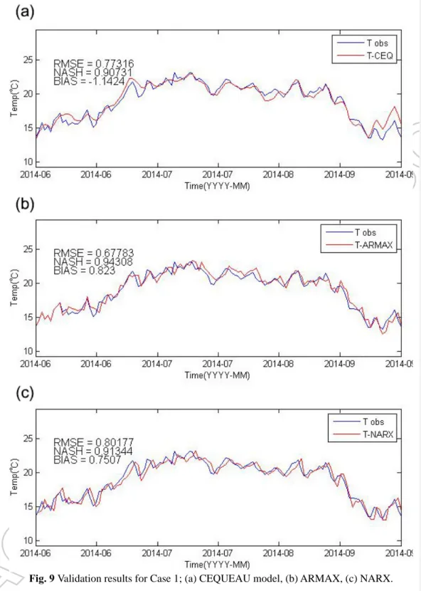
results are shown in Figures 9 and 10 and performance metrics are provided in Table 2. As it is often
the case, all models show higher RMSE and lower Nash coefficient values for the validation than the
calibration phase, except for the CEQUEAU model, which shows similar results for both calibration
Formatted: Font: Not Italic
Formatted: Font: Not Italic
Comment [F12]: replace ‘Nash’ with ‘E’
and validation phases albeit with a higher bias (Table 2). Overall, the ARMAX model has the best
performance, in spite of a slightly higher RMSE and lower NASH value than the deterministic model
during one validation phase (in Case 2, Table 2).
Fig. 9 Validation results for Case 1
:;
(a) CEQUEAU model, (b) ARMAX, (c) NARX.
Fig. 10 Validation results for Case 2; (a) CEQUEAU model, (b) ARMAX, (c) NARX.
Table 2 Calibration and validation performance statistics for each Case.
The CEQUEAU model showed some modeling potential, in spite of a systematic negative
bias (-0.41°C for calibration and -1.06°C for validation phase). It seems that the proximity of the monitoring station to the dam, may be one cause of the bias. The thermal regime in the Fourchue
River is very strongly influenced by the presence of the reservoir. The travelling time is very short
between the dam and the monitoring station (<0.5 day) and thus, the reservoir thermal regime, which
affects the thermal regulation in the lower reach of the Fourchue River, may come into play. For
instance, there may be some occasional stratification and mixing of the water column in the reservoir
that may modulate the temperature of the discharged water. Such an affect is not accounted for by
CEQUEAU. In order to account for stratification, CEQUEAU would need to be coupled to a lake or
reservoir temperature model. If stratification were present, it would also affect the ARMAX and
NARX models. However, in spite of the fact that water was drawn from the reservoir epilimnion,
stratification and mixing may have been an occasional source of error.
Also, in the validation result of Case 2 (Figure 10), all of the selected models, except
CEQUEAU show highly over and under estimated water temperatures between August 27 August, 2011 to and September 8,September 2011 (Figure 10(b) and 10(c)). The high rainfall-runoff events in 2011 seem to be one of the causes of this discrepancy (Figure 4).
Given their autoregressive structure, the ratio of the training sample size to the number of
weights is 29 (Wang et al., 2005) and overfitting may have occurred for ARMAX and NARX during
the calibration phase in Case 2. If this is the case, these models may lack the required robustness to be
operationally implemented. Longer time series would be required to fully investigate this. This
phenomenon shows the potential disadvantage of the statistic and stochastic models. The CEQUEAU
model shows worse results than ARMAX and NARX model, but its performance is more constant
throughout the calibration and validation periods, with 0.8°C in RMSE and 0.9 in Nash coefficient
(Table 2). Otherwise, the deterministic model (CEQUEAU) will be good alternative when the
hydro-climatic data has extreme events which are expected as the cause of overfitting issue.
CONCLUSIONS
This study performed a comparative analysis of three models used to simulate water
temperatures in the Fourchue River, Quebec, Canada. The main conclusions are:
1. As shown by the result of test statistics, water temperature data and most input variables
of the Fourchue River were proven to be chaotic, nonlinear and stochastic time series.
Simple statistic models such as linear regression may prove to be inadequate. For this
reason, more sophisticated time series models (ARMAX and NARX) were tested.
2. The CEQUEAU showed weaker performances than ARMAX and NARX, with
systematic bias. But its performance is constant throughout with 0.8°C in RMSE and 0.9
in Nash coefficient and there is no indication of overfitting.
3. The fact that the ARMAX model proved to have the best performance is not surprising,
given the non-linear autoregressive nature of the model. Water temperatures in any river
have strong autocorrelation. This phenomenon is exacerbated in the Fourchue River,
because of the presence of the reservoir, which has a strong dampening effect.
4. Two models except CEQUEAU show potential overfitting, as shown by their weaker
performance in the validation phase in Case 2. Therefore, the CEQUEAU model
(deterministic approach) will expect the stable performance for the Fourchue River.
Acknowledgements
This work was supported by the NSERC HYDRONET strategic network.
References
Ahmadi‐Nedushan, B., St‐Hilaire, A., Ouarda, T. B., Bilodeau, L., Robichaud, E., Thiemonge, N. and Bobee, B., 2007. Predicting river water temperatures using stochastic models: case study of
the Moisie River (Québec, Canada). Hydrological Processes, 21(1), 21-34.
Ba, K. M., Quentin, E., Carsteanu, A. A., Ojeda-Chihuahua, I., Diaz-Delgado, C. and Guerra-Cobian,
V. H., 2009. Modelling a large watershed using the CEQUEAU model and GIS: The case of
the Senegal River at Bakel. In EGU General Assembly Conference Abstracts, 11, 11839.
Bartholow, J.M., 1995. The stream network temperature model (SNTEMP): A decade of results.
Workshop on Computer Application in Water Management. Fort Collins, Co: Water Resources
Research Institute, CSU. U.S. Geological Survey.
Battiti, R., 1994. Using mutual information for selecting features in supervised neural net learning.
IEEE Transactions on Neural Networks, 5(4), 537–550.
Battiti, R., 1989. Accelerated backpropagation learning: Two optimization methods, Complex systems,
3(4), 331-342.
Bask, M. and Gençay, R., 1998. Testing chaotic dynamics via Lyapunov exponents. Physica D:
Nonlinear Phenomena, 114(1), 1-2.
Beschta, R. L., Bilby, R. E., Brown, G. W., Holtby, L. B. and Hofstra, T. D., 1987. Stream temperature
and aquatic habitat: fisheries and forestry interactions. Streamside management: forestry and
fishery interactions, 57, 191-232.
Benyahya, L., St-Hilaire, A., Quarda, T. B., Bobée, B. and Ahmadi-Nedushan, B., 2007a. Modeling of
water temperatures based on stochastic approaches: case study of the Deschutes
River. Journal of Environmental Engineering and Science, 6(4), 437-448.
Benyahya, L., Caissie, D., St-Hilaire, A., Ouarda, T. B. and Bobée, B., 2007b. A review of statistical
Comment [F13]: if this is financial support, replace heading with ‘Funding’
water temperature models. Canadian Water Resources Journal, 32(3), 179-192.
Benyahya, L., St-Hilaire, A., Ouarda, T. B., Bobee, B. and Dumas, J., 2008. Comparison of
non-parametric and non-parametric water temperature models on the Nivelle River,
France. Hydrological Sciences Journal, 53(3), 640-655.
Beaupré, L., 2014. Comparaison de modèles thermiques statistique et déterministe pour L’estimation
d’indices thermiques sur les portions aménagées et naturelles de la rivière Fourchue (Québec, Canada). Thesis (M. Sc.), INRS-ETE.
Breaker, L. C. and Brewster, J. K., 2009. Predicting offshore temperatures in Monterey Bay based on
coastal observations using linear forecast models. Ocean Modelling, 27(1), 82-97.
Brock, W. A., Dechert, W. D. and Scheinkman, J. A., 1987. A Test for Independence Based on the
Correlation Dimension. Department of Economics, University of Wisconsin at Madison,
University of Houston, and University of Chicago. Social Science Research Working Paper,
8762.
Caldwell, R. J., Gangopadhyay, S., Bountry, J., Lai, Y. and Elsner, M. M., 2013. Statistical modeling
of daily and subdaily stream temperatures: Application to the Methow River Basin,
Washington. Water Resources Research, 49(7), 4346-4361.
Caissie, D., El-Jabi, N. and St-Hilaire, A., 1998. Stochastic modelling of water temperatures in a small
stream using air to water relations. Canadian Journal of Civil Engineering, 25(2), 250-260.
Caissie D., El-Jabi N. and Satish M.G., 2001. Modelling of maximum daily water temperatures in a
small stream using air temperatures. Journal of Hydrology, 251(1), 14–28.
Caissie, D., 2006. The thermal regime of rivers: a review. Freshwater Biology, 51(8), 1389-1406.
Caissie, D., Satish, M. G. and El-Jabi, N., 2007. Predicting water temperatures using a deterministic
model: application on Miramichi River catchments (New Brunswick, Canada). Journal of
Hydrology, 336(3), 303-315.
Chang, H., 2000. Spatial analysis of water quality trends in the Han River basin, South Korea. Water
Research, 42(13), 3285-3304.
Chenard, J.F. and Caissie, D., 2008. Stream temperature modelling using artificial neural networks:
application on Catamaran Brook, New Brunswick, Canada. Hydrologic Process. 22(17),
3361–3372.
Coutant C.C., 1999. Perspective on Temperature in the Pacific Northwest’s Fresh Water.
Environmental Sciences Division, Oak Ridge National Laboratory, ORNL/TM-1999/44. Oak
Ridge National Laboratory, Oak Ridge, Tennessee, 109.
Cover, T. M. and Thomas, J. A., 2006. Elements of information theory. Hoboken, NJ, USA: John
Wiley & Sons, Inc.. http://dx.doi.org/10.1002/047174882X.
Crisp D.T. and Howson G., 1982. Effect of air temperature upon mean water temperature in streams
in the north Pennines and English Lake District. Freshwater Biology, 12(4), 359–367.
Danner, E. M., Melton, F. S., Pike, A., Hashimoto, H., Michaelis, A., Rajagopalan, B. and Nemani, R.
R., 2012. River temperature forecasting: A coupled-modeling framework for management of
river habitat. Selected Topics in Applied Earth Observations and Remote Sensing, IEEE
Journal, 5(6), 1752-1760.
DeWeber, J. T. and Wagner, T., 2014. A regional neural network ensemble for predicting mean daily
river water temperature. Journal of Hydrology, 517(1), 187-200.
Diversi, R., Guidorzi, R. and Soverini, U., 2011. Identification of ARMAX models with noisy input
and output. In World Congress, 18(1), 13121-13126.
Diaconescu, E., 2008. The use of NARX neural networks to predict chaotic time series. WSEAS
Transactions on Computer Research, 3(3), 182-191.
Dibike, Y. B. and Coulibaly, P., 2005. Hydrologic impact of climate change in the Saguenay
watershed: comparison of downscaling methods and hydrologic models. Journal of
hydrology, 307(1), 145-163.
Eleuch, S., Carsteanu, A., Bâ, K., Magagi, R., Goïta, K. and Diaz, C., 2010. Validation and use of
rainfall radar data to simulate water flows in the Rio Escondido basin. Stochastic
Environmental Research and Risk Assessment, 24(5), 559-565.
Gao, Y. and Er, M. J., 2005. NARMAX time series model prediction: feedforward and recurrent fuzzy
neural network approaches. Fuzzy sets and systems, 150(2), 331-350.
Grbi• , R., Kurtagi• , D. and Sliakovi• , D., 2013. Stream water temperature prediction based on
Gaussian process regression. Expert Systems with Applications, 40(18), 7407-7414.
Guillemette, N., A. St-Hilaire, TBMJ Ouarda, N. Bergeron, E. Robichaud et L. Bilodeau., 2009.
Feasibility study of a geostatistical model of monthly maximum stream temperatures in a
multivariate space. Journal of hydrology 364(1), 1-12.
Handeland, S. O., Imsland, A. K. and Stefansson, S. O., 2008. The effect of temperature and fish size
on growth, feed intake, food conversion efficiency and stomach evacuation rate of Atlantic
salmon post-smolts. Aquaculture, 283(1), 36-42.
Haykin, S., 1999. Neural networks: a comprehensive foundation (second ed.), Prentice hall, Upper
Saddle River, New Jersey, USA.
Hammitt, W. E. and Cole, D. N., 1998. Wildland recreation: ecology and management. John Wiley &
Sons, Hoboken, NJ, USA.
Hadzima-Nyarko, M., Rabi, A. and Šperac, M., 2014. Implementation of Artificial Neural Networks
in Modeling the Water-Air Temperature Relationship of the River Drava. Water Resources
Management, 28(5), 1379-1394
Hyndman, R. J., and Khandakar, Y., 2006. Automatic time series for forecasting: the forecast package
for R (No. 6/07). Monash University, Department of Econometrics and Business Statistics
Jeppesen E. and Iversen T.M., 1987. Two simple models for estimating daily mean water temperatures
and diel variations in a Danish low gradient stream. Oikos, 49(1), 149–155.
Jeong, D. I., Daigle, A. and St‐Hilaire, A., 2013. Development of a stochastic water temperature model and projection of future water temperature and extreme events in the Ouelle River
basin in Québec. Canada. River Research and Applications, 29(7), 805-821.
Johnson F.A., 1971. Stream temperatures in an alpine area. Journal of Hydrology, 14(3), 322–336.
Jose M. P. Menezes Jr. and Barreto, G. A., 2008. Long-term time series prediction with the NARX
network: An empirical evaluation. Neurocomputing, 71(16), 3335-3343
Jourdonnais J.H., Walsh R.P., Pickett F. and Goodman D., 1992. Structure and calibration strategy for
a water temperature model of the lower Madison River, Montana. Rivers, 3(3), 153–169.
Kim K.S. and Chapra S.C., 1997. Temperature model for highly transient shallow streams. Journal of
Hydraulic Engineering, 123(1), 30-40.
Kothandaraman, V., 1972. Air-water temperature relationshop in illinois. Journal of the American
Water Resources Association, 8(1), 38-45.
Larnier, K., Roux, H., Dartus, D. and Croze, O., 2010. Water temperature modeling in the Garonne
River (France). Knowledge and Management of Aquatic Ecosystems, 398(1), 4.
Lessard, J. L. and Hayes, D. B., 2003. Effects of elevated water temperature on fish and
macroinvertebrate communities below small dams. River research and applications, 19(7),
721-732.
Levene, Howard, 1960. Contributions to Probability and Statistics: Essays in Honor of Harold
Hotelling. Stanford University Press. 278–292.
Lin, T., Horne, B. G., Tiño, P. and Giles, C. L., 1996. Learning long-term dependencies in NARX
recurrent neural networks, IEEE Trans. Neural Networks, 7(6), 1329–1338.
Ljung G. M. and G. E. P. Box, 1978. On a Measure of a Lack of Fit in Time Series
Models. Biometrika, 65(2), 297–303.
Mackey, A. P. and Berrie, A. D., 1991. The prediction of water temperatures in chalk streams from air
temperatures. Hydrobiologia, 210(3), 183-189.
Maier, H. R. and Dandy, G. C., 2000. Neural networks for the prediction and forecasting of water
resources variables: a review of modelling issues and applications. Environmental Modelling
& Software, 15(1), 101–124.
May, R. J., Dandy, G. C., Maier, H. R. and Nixon, J. B., 2008. Application of partial mutual
information variable selection to ANN forecasting of water quality in water distribution
systems. Environmental Modelling & Software, 23(10), 1289-1299.
Mestekemper, T., Windmann, M. and Kauermann, G., 2010. Functional hourly forecasting of water
temperature. International Journal of Forecasting, 26(4), 684-699.
Mohseni O., Stefan H.G. and Erickson T.R., 1998. A nonlinear regression model for weekly stream
temperatures. Water Resources Research, 34(10), 2685–2692.
Mohseni O. and Stefan H.G., 1999. Stream temperature/air temperature relationship: a physical
interpretation. Journal of Hydrology, 218(3), 128–141.
Moriasi, D. N., Arnold, J. G., Van Liew, M. W., Bingner,R. L., Harmel, R. D., Veith, T. L.,
2007. Model Evaluation Guidelines for Systematic Quantification of Accuracy in Watershed
Simulations. Transactions of the ASABE, 50 (3), 885–900.
Morin, G. and Slivitzky, M., 1992. Impacts of climatic changes on the hydrological regime: Moisie
river case. Revue des sciences de l'eau/journal of water science, 5(2), 179-195.
Morin G, Fortin JP, Lardeau JP, Sochanska W. and Paquette S., 1981. Mode`le CEQUEAU: manuel
d’utilisation. INRS-Eau, Ste-Foy, Que´bec, Canada
Morin G, Sochanski W., Paquet P., 1998. Le mode`le de simulation de quantite´ CEQUEAU-ONU,
Manuel de re´fe´rences. Organisation des Nations-Unies et INRS-Eau. Rapport de recherche
no. 519, 252.
Morin G. and Paquet P., 2007. Mode`le hydrologique CEQUEAU, INRS-ETE, rapport de recherche
no. R000926, 458.
Morrill, J. C., Bales, R. C. and Conklin, M. H., 2005. Estimating stream temperature from air
temperature: implications for future water quality. Journal of Environmental
Engineering, 131(1), 139-146.
Morse, W. L., 1970. Stream temperature prediction model. Water Resources Research, 6(1), 290-302.
Myers, Jerome L.; Well, Arnold D., 2003. Research Design and Statistical Analysis (2nd ed.).
Lawrence Erlbaum. 508. ISBN 0-8058-4037-0.
Nash, J. E. and J. V. Sutcliffe, 1970. River flow forecasting through conceptual models part I — A
discussion of principles. Journal of Hydrology, 10 (3), 282–290.
Nowak, K., J. Prairie, B. Rajagopalan and U. Lall, 2010. A nonparametric stochastic approach for
multisite disaggregation of annual to daily streamflow. Water Resources Research, 46,
W08529, doi:10.1029/2009WR008530.
Nunn, A. D., Cowx, I. G., Frear, P. A. and Harvey, J. P., 2003. Is water temperature an adequate
predictor of recruitment success in cyprinid fish populations in lowland rivers?, Freshwater
Biology, 48(4), 579-588.
Ojanguren, A. F., Reyes-Gavilán, F. G. and Braña, F., 2001. Thermal sensitivity of growth, food intake
and activity of juvenile brown trout. Journal of thermal biology, 26(3), 165-170.
Pal'shin, N. I. and Efremova, T. V., 2005. Stochastic Model of the Annual Cycle of Water Surface
Temperature in Lakes. Russian Meteorology and Hydrology, 3(1), 61-68.
Pike, A., Danner, E., Boughton, D., Melton, F., Nemani, R., Rajagopalan, B. and Lindley, S., 2013.
Forecasting river temperatures in real time using a stochastic dynamics approach. Water
Resources Research, 49(9), 5168-5182.
Sahoo, G. B., Schladow, S. G. and Reuter, J. E., 2009. Forecasting stream water temperature using
regression analysis, artificial neural network, and chaotic non-linear dynamic models. Journal
of Hydrology, 378(3), 325-342.
Sauquet, E., Dupeyrat, A., Perrin, C., Agosta, C., Hendrickx, F. and Vidal, J. P., 2009. Impact of
business-as-usual water management under climate change for the Garonne catchment
(France). In IOP Conference Series: Earth and Environmental Science, 6(29), 292009.
Seiller, G. and Anctil, F., 2014. Climate change impacts on the hydrologic regime of a Canadian river:
comparing uncertainties arising from climate natural variability and lumped hydrological
model structures. Hydrology and Earth System Sciences, 18(6), 2033-2047.
Selong, J. H., McMahon, T. E., Zale, A. V. and Barrows, F. T., 2001. Effect of temperature on growth
and survival of bull trout, with application of an improved method for determining thermal
tolerance in fishes. Transactions of the American Fisheries Society, 130(6), 1026-1037.
Singh, K. P., Malik, A., Mohan, D. and Sinha, S., 2004. Multivariate statistical techniques for the
evaluation of spatial and temporal variations in water quality of Gomti River (India)—a case
study. Water research, 38(18), 3980-3992.
Sinokrot B.A. and Stefan H.G., 1993. Stream temperature dynamics: measurements and modeling.
Water Resources Research, 29(7), 2299-2312.
Stefan, H. G. and Preud'Homme, E. B., 1993. Stream temperature estimation from air
temperature. Journal of the American Water Resources Association, 29(1), 27-45.
St-Hilaire, A., Morin, G., El-Jabi, N. and Caissie, D., 2000. Water temperature modelling in a small
forested stream: implication of forest canopy and soil temperature. Canadian Journal of Civil
Engineering, 27(6), 1095-1108.
St‐Hilaire, A., El‐Jabi, N., Caissie, D., and Morin, G., 2003. Sensitivity analysis of a deterministic
water temperature model to forest canopy and soil temperature in Catamaran Brook (New
Brunswick, Canada). Hydrological processes, 17(10), 2033-2047.
St‐Hilaire, A., Ouarda, T. B., Bargaoui, Z., Daigle, A. and Bilodeau, L., 2012. Daily river water temperature forecast model with ak‐nearest neighbour approach. Hydrological
Processes, 26(9), 1302-1310.
St‐Hilaire, A., Ouarda, T. B., Bargaoui, Z., Daigle, A. and Bilodeau, L., 2012. Daily river water temperature forecast model with ak‐nearest neighbour approach. Hydrological
Processes, 26(9), 1302-1310.
Wang, D. and Huang, J., 2005. Neural network-based adaptive dynamic surface control for a class of
uncertain nonlinear systems in strict-feedback form. Neural Networks, IEEE Transactions on,
16(1), 195-202.
Webb, B. W., Hannah, D. M., Moore, R. D., Brown, L. E. and Nobilis, F., 2008. Recent advances in
stream and river temperature research. Hydrological Processes, 22(7), 902-918.
Younus M., Hondzo M. and Engel B.A., 2000. Stream temperature dynamics in upland agricultural
watershed. Journal of Environmental Engineering, 126(1), 518–526
[Table 1. Test statistics for each dependent and independent variables
.;
W(m)
: indicated
embedding dimension
;,
95% C.I.
: indicated
95% confidential inbound for test
;
and
rejected
data
are
marked
as in
bold
character
].
Test Stat. Value
Dependent and independent variables
Water Temp. of Upstream Water Temp. of Downstream (Target) Air Temp. Runoff from Fourchue Ddam Solar Radiation Relative humidity Average Wind Speed Levene’s test p-value 0.448 0.877 0.548 0.000 0.239 0.992 0.657 Lyapunov exponent Lamda test calculated 1.82 x 10⁻⁶ 1.62 x 10⁻⁶ 0.000 1.000 0.0003 0.274 0.000 95% C.I. -0.0653 -0.1486 -0.3825 0.1245 -0.1868 -0.2372 -0.6811 BDS test W(2) 79.02 62.15 20.96 16.49 2.82 19.58 2.53 W(3) 85.80 67.11 20.30 15.17 0.81 18.29 2.42 W(4) 94.52 73.32 19.81 13.79 0.46 17.12 2.05 W(5) 106.87 82.27 19.86 12.74 0.54 16.62 1.74 95% C.I [-1.96, +1.96] Result Nonlinear stochastic time series Nonlinear stochastic time series Nonlin ear stochas tic time series Chaotic time series with hetero-skedastici ty Random series Chaotic time series Nonlinear stochastic time series
Comment [F14]: Please edit tables: -remove [ ] from the caption and remove bold and italics (I have done Table 1 caption)
-remove shading/colour and all lines except horizontal line above and below the table and below the header row
remove upper case initials except for the first word in each heading unless proper noun, e.g. Dam
Formatted: Font: Not Bold Formatted: Font: Not Italic Formatted: Font: Not Italic Formatted: Font: Not Italic Formatted: Font: Not Italic Formatted: Font: Not Italic
Formatted: Font: Not Italic Formatted: Font: Not Italic Comment [F15]: editing tables:
-remove [ ] from the caption and remove bold and italics
-remove shading/colour and all lines except horizontal line above and below the table and below the header row
-remove upper case initials except for the first word in each heading unless proper noun, e.g. Dam
[Table 2. Calibration and validation performance statistics for each Case]
CASE Model
Calibration phase Validation phase
RMSE(°C) NASH BIAS(°C) RMSE(°C) NASH BIAS(°C)
CASE 1 CEQUEAU 0.80 0.91 -0.36 0.77 0.91 -1.14 ARMAX 0.57 0.96 0.04 0.68 0.94 0.82 NARX 0.67 0.94 0.11 0.80 0.91 0.75 CASE 2 CEQUEAU 0.78 0.92 -0.45 0.83 0.88 -0.97 ARMAX 0.55 0.96 0.01 1.14 0.83 1.60 NARX 0.65 0.94 -0.18 1.46 0.77 4.20 Overall Result CEQUEAU 0.79 0.92 -0.41 0.80 0.90 -1.06 ARMAX 0.56 0.96 0.03 0.91 0.89 1.21 NARX 0.66 0.94 -0.18 1.13 0.84 2.48
Fig. 1 Study area and measuring station.
Comment [F16]: please see edits to figure captions in the main body textFig. 2 Hydro-physiographical characteristics of study area. Map shows land use, whole
squares (elementary hydrological units) and arrows indicate water routing used for the
deterministic (CEQUEAU) model.
Comment [F17]: in fig. 2, after Datum: North, you have spelled American incorrectly (Amreican)

![Fig. 1 Study area and measuring station. Comment [F16]: please see edits to figure captions in the main body text](https://thumb-eu.123doks.com/thumbv2/123doknet/2941990.79267/24.892.102.672.205.1029/fig-study-measuring-station-comment-edits-figure-captions.webp)