To link to this article : DOI :
10.1016/j.ultras.2015.11.003
URL :
https://doi.org/10.1016/j.ultras.2015.11.003
To cite this version :
Szasz, Teodora and Basarab, Adrian and Kouamé,
Denis Strong reflector-based beamforming in ultrasound medical imaging.
(2016) Ultrasonics, vol. 66. pp. 111-124. ISSN 0041-624X
O
pen
A
rchive
T
OULOUSE
A
rchive
O
uverte (
OATAO
)
OATAO is an open access repository that collects the work of Toulouse researchers and
makes it freely available over the web where possible.
This is an author-deposited version published in :
http://oatao.univ-toulouse.fr/
Eprints ID : 16872
Any correspondence concerning this service should be sent to the repository
administrator:
staff-oatao@listes-diff.inp-toulouse.fr
Strong reflector-based beamforming in ultrasound medical imaging
Teodora Szasz
⇑, Adrian Basarab, Denis Kouamé
Université de Toulouse, IRIT, UMR CNRS 5505, FranceKeywords:
Adaptive beamforming Sparse signal representation Ultrasound imaging Bayesian Information Criteria
a b s t r a c t
This paper investigates the use of sparse priors in creating original two-dimensional beamforming methods for ultrasound imaging. The proposed approaches detect the strong reflectors from the scanned medium based on the well known Bayesian Information Criteria used in statistical modeling. Moreover, they allow a parametric selection of the level of speckle in the final beamformed image. These methods are applied on simulated data and on recorded experimental data. Their performance is evaluated considering the standard image quality metrics: contrast ratio (CR), contrast-to-noise ratio (CNR) and signal-to-noise ratio (SNR). A comparison is made with the classical delay-and-sum and minimum variance beamforming methods to confirm the ability of the proposed methods to precisely detect the number and the position of the strong reflectors in a sparse medium and to accurately reduce the speckle and highly enhance the contrast in a non-sparse medium.
We confirm that our methods improve the contrast of the final image for both simulated and experi-mental data. In all experiments, the proposed approaches tend to preserve the speckle, which can be of major interest in clinical examinations, as it can contain useful information. In sparse mediums we achieve a highly improvement in contrast compared with the classical methods.
1. Introduction
Ultrasound (US) imaging is one of the most commonly used medical imaging modalities. Its low-cost, non-ionizing characteris-tics, ease-of-use and real-time nature makes it the gold standard for many crucial diagnostic exams, especially in obstetrics and cardiology.
Beamforming (BF) or spatial filtering[1]enables the selectivity
of the acoustic signals reflected from some known positions, while attenuating the signals from other positions. This is classically done by delaying and applying some specific weights to the reflected signals. The applications of BF are versatile to many areas: radar, sonar, imaging, communications, radio astronomy and others. The beamformers can be either data-independent (fixed), or data-dependent (adaptive), depending on the calculation of the weights applied to the output array of the reflected signals. The simplest yet most used data-independent BF method in US imaging is the classical delay-and-sum (DAS) BF, which uses fixed apodization weights to approximate the array response indepen-dent of the array data. Unfortunately, the resolution and the con-trast achievable with DAS are limited. On the other hand, the adaptive beamformers calculate the weights from the statistics of the received data in order to converge to an optimal response.
Thus, the contributions of the noise and the signals that arrive from other directions than the desired one are minimized.
The data-dependent beamformers offer a better resolution and a higher interference rejection capability if the signal of interest (SOI) and the true covariance matrix are accurately known. Differ-ent data-dependDiffer-ent approaches may be found in literature. Capon introduced the widely used Capon or minimum variance (MV)
beamformer[2], which minimizes the power of the weighted array
data such that the desired signal passes without distortion. How-ever, in practice, just an estimation of the covariance matrix can be provided, which can be ill-conditioned, providing worst results than the fixed BF methods. In consequence, more robust adaptive
beamformers have been developed. Bell et al.[3]proposed a
Baye-sian approach, robust to uncertainty of the direction of arrival (DOA) of the source. More recently, Li and Stoica proposed a spher-ical set constrained on the beamformer steering vector, using also the popular diagonal loading approach for improving the
robust-ness of the Capon beamformer[4].
In medical US imaging, Asl et al. combined MV with diagonal
loading and phase coherence factor (see e.g.[5,6]) to achieve better
results than DAS in terms of lateral resolution, sidelobes reduction and contrast. Another approach proposed by Holfort et al. uses fre-quency subbands and calculates a set of complex apodization
weights for each frequency subband[7]. They argue an increase
of contrast and lateral resolution even in the case of plane-wave ⇑ Corresponding author.
US imaging (when only one emission is used). Recently, Diamantis et al. provide a comparison between the temporal and frequency subband approaches of MV for US images and show that there are insignificant differences in terms of spatial resolution and
con-trast[8]. Moreover, Rindal et al. contest the improvement in
con-trast related to MV, and show that this is the result of the
increase in lateral resolution[9].
A new perspective in adaptive BF was recently exploited, based on sparse representation of the signals. Yartibi et al. proposed two user parameter-free BF approaches for estimating source locations in array processing: the iterative adaptive approach (IAA) and the
maximum likelihood based IAA (IAA-ML)[10,11]. These methods
take as input the result of DAS and, using an iterative algorithm, minimize the weighted least squares (WLS) cost function in order to estimate the signal powers.
Sparse modeling gained a special interest in medical US, as for example in modeling the amplitude of the potential reflectors by using an iterative adaptive approach (IAA) present in array
pro-cessing literature[12]. Other examples can be the applications that
concern compressive sensing [13]. Tur et al. model the echoes
reflected by multiple reflectors located at unknown positions in the medium, as a sum of a small number of pulses with known
shapes [14]. Based on this, Wagner et al. proposed a
two-dimensional reconstruction method for US imaging, called
‘‘compressed beamforming” [15]. They used multiple array
elements in receive and beamformed the sub-Nyquist received samples.
In our preliminary work[16], we obtained a sparse signal
rep-resentation by extending the DAS BF method with BIC (Bayesian Information Criteria) selection criteria. Here, we improve the pre-viously proposed method in order to obtain more realistic results in terms of speckle conservation. Moreover, we extend MV BF method with BIC in order to exploit the advantages of the MV BF to our sparse modeling. Finally, we propose a new method that computes the final beamformed image by combining the sparse representation with the DAS and MV beamformed results. Com-pared with DAS and MV, we increase the contrast while preserving the speckle (that frequently contain important clinical informa-tion) in the final beamformed image.
The reminder of this paper is as follows: in Section 2 we
describe the background of DAS and MV BF method. In Section3
we present the proposed method that was validated both on pulse echo simulated ultrasound data and real ultrasound phantom data recorded with an Ultrasonix MDP scanner. A detailed description of
the experiments is given in Section4. Section5presents the results
and Section6concludes the paper.
2. Background on US beamforming
Throughout this paper, we denote the vectors and the matrices with boldface lowercase, respectively with boldface capital letters. InTable 1we describe the notations used in this paper.
The basic principle of US imaging consists in emitting US waves with a probe towards a target medium and receiving the reflected (or backscattered) waves (echoes) resulting from the interaction between US waves and the tissues. These acquired signals (raw data) are delayed, weighted using apodizations and summed to obtain the radio-frequency (RF) signals. The most used method to display an US image is the B-mode and consists in extracting the envelope of the RF signals, filtering and log-compressing.
Assuming an M-element ultrasound probe, we consider here-after the classical acquisition scheme, where a series of focused
beams is transmitted with Mact elements. The raw signals are
recorded using the same subarray that was used for transmission. The DAS beamformed RF signals can be written as:
^siðnÞ ¼ wHðnÞyðiÞdðnÞ ¼
XMact
k¼1
wkðnÞyðiÞkðn $
D
kðnÞÞ n ¼ 1; . . . ; N; ð1Þwhere N is the number of samples of the RF signal, yðiÞ
k is the 1 % N
raw data received by the k-th element of the ultrasound probe
cor-responding to emission number ðiÞ;DkðnÞ is the time delay
depen-dent on the distance between the k-th element and the point of
interest in the image, wk are the beamformer weights,
yðiÞdðnÞ 2 RMact%1; yðiÞ
dðnÞ ¼ yðiÞðn $DkðnÞÞ is the dynamically focused
version of the raw data yðiÞðnÞ ¼ ½yðiÞ
1ðnÞ; . . . ; y ðiÞ MactðnÞ( T ; wðnÞ ¼ ½w1; . . . ; wMact( T
is the vector of the beamformer weights, ð)ÞT and
ð)ÞHrepresent the transpose and conjugate transpose, respectively.
Without loss of generality, for simplicity purpose, we consider throughout the theoretical part that the number of the beamformed RF lines is equal to M.
While the DAS beamformer uses fixed data-independent weights w, the aim of MV is to apply an optimal set of weights in order to estimate the desired signal waveform as accurately as possible, while rejecting the interfering signals. The optimal weights in the sense of MV, can be obtained from the expression
of the signal-to-interference-plus-noise ratio (SINR)[17]:
SINR ¼
r
2 sjwHaj
2
wHRw ; ð2Þ
where R of size Mact% Mactis the interference-plus-noise covariance
matrix,
r
2s is the signal power and a the steering vector. To have a
maximum SINR, the output interference-plus-noise power is mini-mized, while maintaining a distortionless response to the desired signal: min w w HRw; subject to wHa ¼ 1: ð3Þ Table 1
Mathematical notations used in the paper. Notation Explanation
M Number of elements of the probe
Mact Number of active elements in emission and reception N Number of samples of each RF signal
YðiÞ Raw data of size Mact% N corresponding to the ith pulse emission YðiÞd Dynamically focused raw data of size Mact% N corresponding to
the ith pulse emission
w Beamformer weight vector of size 1 % Mact wh Hanning window of size 1 % Mact R Covariance matrix
^
R Estimated covariance matrix yðiÞ
k Non-focused raw signal of size 1 % N received by the k-th element, corresponding to emission k
yðiÞ
d Focused raw signal of size 1 % N ^
S DAS beamformed image of size M % N ^si ith DAS beamformed RF signal of size 1 % N ~
S MV beamformed image of size M % N ~si ith MV beamformed RF signal of size 1 % N si USBIC or M-USBIC beamformed RF signal SðKÞ USBIC or M-USBIC sparse beamformed image
SUSBIC Final USBIC beamformed image with speckle
SM$USBIC Final M-USBIC beamformed image with speckle
k Parameter for setting the sparsity level c Parameter for setting the speckle level ð)ÞT Transpose of a vector or matrix ð)ÞH Conjugate transpose of a vector or matrix + Hadamard product of two vectors/matrices f1DðkÞ Cost function for 1D BIC approach f2DðkÞ Cost function for 2D BIC approach k ) k2 l2-norm
1> Is the transpose of a all-ones matrix K Number of strong reflectors
After applying the proper delays to the raw data, a becomes a
vector of ones. Therefore, the solution of(3), also called the
mini-mum variance distortionless response beamformer (a is the steer-ing vector across the array), is:
~ w ¼ R
$1a
aHR$1a: ð4Þ
As in practical situation the analytical form of R is not known, it is usually replaced by the estimated covariance matrix derived
from P received samples, denoted by ^R:
^ R ¼1 P XP p¼1 yðiÞ dðpÞy ðiÞ d ðpÞ H : ð5Þ
In order to decorrelate the coherent signals received from the
Mact elements, the subarray-averaging method is generally used.
Specifically, the Mact element linear array is divided into
Mact$ L þ 1 overlapping subarrays of size L, and the covariance
matrices from L subarrays are averaged [18]. However, it was
shown that in this case the tissue may appear less homogeneous
and may give different statistics compared with DAS[19]. To retain
the speckle statistics, the temporal averaging was introduced in
[20]. By averaging both in the spatial (lateral direction) and
tempo-ral domains, the resolution can be further improved, with no con-trast degradation. Finally, the MV beamformer output can be expressed as: ~siðnÞ ¼ 1 Mact$ L þ 1 X Mact$Lþ1 l¼1 ~ wHðnÞyðiÞðlÞ d ðnÞ; i ¼ 1; . . . ; M; ð6Þ where yðiÞðlÞ
d ðnÞ is the dynamically focused raw data corresponding to
the l-th subarray of size L.
3. Beamforming with sparse priors: proposed method
Based on the beamforming methods reviewed in the previous section (DAS and MV), the proposed method consists in detecting and reinforcing the strong reflectors in the RF images. In practice, these reflectors may be associated to the tissue boundaries or the
small hyperechoic structures (see e.g.[14,15]).
As we will explain below, the strong reflector detection is based on the minimization of the Bayesian Information Criteria (BIC), bal-ancing between data fidelity and a sparsity-based penalization
term[21].
3.1. Sparse strong reflector model
The strong reflector model of an RF image S, considered herein as a collection of M RF lines each one having N samples, is given as:
Sðx; nÞ ¼X K k¼1 akhkðx $ xk; n$ nkÞ; x ¼ x1; . . . ; xM and n ¼ 1; . . . ; N; ð7Þ
where n stands for the time or axial (longitudinal) direction, x is the lateral direction variable, and Sðx; nÞ is the beamformed RF image.
ðxk; nkÞ, with k ¼ 1; . . . ; K are the positions of the K strong reflectors
to be detected during the proposed beamforming process. We
denote with ak the amplitudes of the strong reflectors and with
hkðx; nÞ the backscattered pulse corresponding to the strong
reflec-tor k, both supposed unknown and to be estimated. In this case the term sparsity is related to the relatively low number of strong reflectors to be detected by the proposed method.
3.2. Strong reflector detection and parameter estimation
In this section, we describe the proposed process of strong reflector detection and parameter estimation. The proposed method is mainly divided in two steps: the detection step, based on the previously beamformed RF lines, finds the strong reflectors taking into account the amplitudes of the RF signals. Then, the val-idation step uses the raw data to confirm the previously detected reflectors through the BIC criteria. The main reason of processing the detection of the strong reflectors on beamformed data instead of raw data is related to the SNR that is naturally higher on stan-dardly beamformed data compared to raw data. Thus, we expect that the results are less affected by the low SNR when detecting the peaks on DAS or MV images.
For the ease of understanding, we use the same notations as in
Section2, corresponding to a classical pulse echo US image. The
raw data is collected with the corresponding Mactactive elements,
resulting into a data matrix of size Mact% N, denoted by YðiÞd. More
precisely, yðiÞ
dðnÞ is a Mact% 1 line corresponding to emission
num-ber ðiÞ and to depth n, after the dynamic focalisation of the received echoes.
As explained in Section2, the total amount of raw data is used
in non-adaptive BF process to obtain the DAS beamformed RF
image denoted by ^S, or in an adaptive BF process to form the MV
beamformed RF image denoted by ~S. We denotes^i, and ~sithe ith
RF signals extracted from ^S, respectively ~S. Our strong reflector
detection and parameter estimation method uses both the raw
data YðiÞ
d, and the beamformed RF images ^S or ~S. Both proposed
approaches, using the DAS or MV beamformed RF images, are sim-ilar and will be referred as USBIC, respectively M-USBIC in the reminder of the paper.
Two main steps are used within the proposed method. The first
step uses ^S or ~S to detect a potential strong reflector (its position,
amplitude, and pulse response). The second step validates this choice and estimation based on a cost function implying the raw data. The first and the second steps are alternatively repeated until the algorithm stops (the minimum of BIC is reached). Moreover, an initial one-dimensional (1D) approach is followed by a two-dimensional (2D) refinement, both using the two aforementioned steps. In the following, we describe only the steps required to form
the USBIC beamformed RF image (denoted with SðKÞin the paper).
In this case we use as input the DAS beamformed RF image ^S, and
the raw data YðiÞ
d. The steps to form the M-USBIC beamformed RF
image (when the MV beamformed RF image ~S and the YðiÞd are
the inputs) are identical with the ones required to form USBIC beamformed RF image.
3.2.1. 1D initialization procedure
For each beamformed RF line ^siat lateral position xithe strong
reflector detection and validation are iterated. For iteration k, the two steps are process as follows:
Step 1 – Strong reflector detection.
nk¼ argmax nnfn1;...;nk$1g ðj^siðnÞjÞ; ak¼ j^siðnkÞj; hkðxi; nÞ ¼ ^Sðxi; nÞ + whðnÞ; n ¼ nk$
s
pulse) fs 2 ; . . . ; nkþs
pulse) fs 2 " # ; ð8Þwhere nk is in the interval f1; . . . ; Ng; ^Sðxi; nÞ is the DAS
beam-formed image, wh is a Hanning window,
s
pulse is the predefinedis the sampling frequency, + defines the Hadamard product, and argmax stands for the argument of the maximum. The current form of the detected strong reflector RF signal, after k iterations, is:
sðkÞ i , S ðkÞ ðxi; nÞ ¼ Xk p¼1 aphpðxi; nÞ; ð9Þ where sðkÞ
i is the i-th column of the RF image S
ðkÞ
ðx; nÞ, at the itera-tion k.
Step 2 – Validation. In the second step of each iteration, a cost function is calculated balancing between on the one hand, the data
fidelity between the current RF model in(9)and the raw data and
on the other hand, the sparsity of the strong reflectors. The BIC
evaluation criterion[21]is one of the most used information
crite-ria in statistics, having the role of assessing the closeness between the predictive distribution defined by a statistical model and the true distribution. A statistical model uses the observed data to approximate the true distribution of certain probabilistic events.
Let gð
v
nj^hÞ be a statistical model estimated by the maximumlike-lihood method. Than, the BIC criterion is defined as:
BICðnÞ ¼ $2 log gð
v
nj^hÞ þ p log n; ð10Þwhere h is the unknown parameter, ^h is its estimator, and
v
nare theobservations,
v
n¼ fv
1;v
2; . . . ;v
ng. Inspired from the application ofBIC with IAA for obtaining sparsity by estimating the number of
sources in array processing, described in [11], BIC was adapted
herein to US imaging. The cost function f1DðkÞ has the following
form: f1DðkÞ ¼ logðks ðkÞ i ) 1 > $ yðiÞd k 2 2Þ zfflfflfflfflfflfflfflfflfflfflfflfflfflfflfflfflfflfflffl}|fflfflfflfflfflfflfflfflfflfflfflfflfflfflfflfflfflfflffl{data fidelity þ kk logðNÞ |fflfflfflfflfflffl{zfflfflfflfflfflffl} sparsity constraint ; ð11Þ
where k is an user-defined parameter fixing the compromise between the data attachment and the sparsity. Even if the auto-matic choice of the k is out of the scope of this paper, note that there exist in literature several approaches that automatically determine
the value of this kind of hyperparameter, see e.g.[22–25].
For each RF line, Step 1 and Step 2 are iterated until the cost
function in (11) starts to increase (i.e. f1Dðk þ 1Þ > f1DðkÞ). Note
that the data fidelity term is not related to already beamformed RF lines, but to the raw data (native data received by each element
of the US probe), at each iteration, having the dimension Mact% N.
Let us denote byWthe set of all the strong reflector positions
detected from all individual RF lines. Applied on each RF line, the algorithm tends to overestimate the number of strong reflectors. Moreover and more important, it does not ensure a spatial coher-ence between the neighboring RF lines. For this reason, a 2D approach follows the 1D method, and is presented bellow. It will
choose a subset of strong reflectors ofWrespecting a 2D BIC
crite-ria. The main advantage of applying the 1D approach is to speed up (at least three times in our experiments) the 2D process that will have as input just the potential strong reflectors detected previ-ously by the 1D method for each RF line.
3.2.2. 2D refinement procedure
For the refinement of the previously detected reflectors (by the
1D approach) we use the setW, representing all the strong
reflec-tors positions of all the RF lines. For all strong reflecreflec-tors detected in the 1D approach, an 2D – adapted BIC criteria is applied. The pro-cess of the 2D refinement iteratively gathers the best positions
from the setW, as follows:
nk¼ argmax n2Wnfn1;...;nk$1g
ðanÞ; ð12Þ
where an is expressed in (8). The selected strong reflectors are
plugged into the 2D BIC criteria, given by:
f2DðkÞ ¼ log XM i¼1ks ðkÞ i ) 1 >$ yðiÞ d k 2 2 ) * zfflfflfflfflfflfflfflfflfflfflfflfflfflfflfflfflfflfflfflfflfflfflfflfflfflffl}|fflfflfflfflfflfflfflfflfflfflfflfflfflfflfflfflfflfflfflfflfflfflfflfflfflffl{data fidelity þ kk logðNÞ |fflfflfflfflfflffl{zfflfflfflfflfflffl} sparsity constraint ; ð13Þ where sðkÞ i is defined in(9).
The 2D validation step is iterated until the function f2DðkÞ starts
to increase, similar as for the 1D initialization approach. Moreover,
as stated in Section3.2.1, the data fidelity term for the 2D approach
is composed of all the focused raw data corresponding to all
emis-sions, having the dimension Mact% M % N.
3.3. Final image computation
As we will show in the results section, the method introduced in
Section3.2has a good ability to detect the strong reflectors and to
provide a sparse version of the RF image. However, it does not pre-serve the speckle characteristics, that can contain clinical informa-tion, in the case when the examined medium is not sparse. For this reason, we propose to further combine our sparse RF image with the one that is classically beamformed with DAS or MV, as shown
below. If the DAS RF image ^S is used (for strong reflector detection
and final image combination), we call the resulted image USBIC. If
the MV RF image ~S is used, we call it M-USBIC. Hence, the final
USBIC beamformed image can be expressed as:
SUSBIC¼
c
) bS þ ð1 $c
Þ ) SðKÞ; ð14Þwhere SðKÞ is the beamformed image obtained using our sparse
strong reflector model and is defined in(7),
c
is the parameter thatcontrol the level of speckle in the final image, and K is the number of the strong reflectors detected after the k iterations.
Similar, the M-USBIC has the following expression:
SM$USBIC¼
c
) eS þ ð1 $c
Þ ) SðKÞ ð15ÞNote that SðKÞbe obtained either by using the DAS beamformed
image (in the case of USBIC, or starting from the MV beamformed image (in the case of M-USBIC).
4. Experiments
In order to evaluate the proposed USBIC and M-USBIC BF approaches, we have considered three different simulated
exam-ples using the Field II simulation program[26]and one recorded
ultrasound phantom data. The first simulated medium is based on a sparse assumption of the reflectors. The second one is based on simulated data from scenes of point-targets and scenes of cysts in speckle considering a phased array imaging technique. The third example represents the simulation of a cardiac image (the ampli-tudes of the scatterers were related to the gray levels of an Apical
4 Chambers (A4C) view image, as suggested in[27]). The
experi-mental data was acquired with an Ultrasonix MDP research plat-form. The simulation and experimental parameters are resumed inTable 2.
For all the following examples, the improved version of MV BF
was used, the one that gives the best results in[6], with spatial
averaging with L ¼ Mact=2¼ 32, temporal averaging T ¼ 10, and
the diagonal loading factorD¼ 1=L. The B-mode image
computa-tion was processed in a standard manner and in the same way for all the resulted images: Hilbert-based demodulation and logarithmic compression.
4.1. Simulated point reflectors
A scanned grid with 14 point reflectors was simulated, laterally aligned in pairs of two and separated by 4 mm. They are located at axial depths ranging from 40 to 80 mm, with a transmit focus at 50 mm and a dynamic receive focalisation.
4.2. Simulated point reflectors and cyst data
For this type of simulation the medium was scanned with a
7 MHz 128-element phased array transducer with wa
v
elength=2spacing and Hanning apodization. A two-cycle sinusoidal was used as excitation and the transmit focus was set to 60 mm. We adopted a dynamically receive focalisation ranging from 5 to 150 mm. The images consist in 128 lines with 0.7" between consecutive lines. The medium consists in several circular cysts: an anechoic one with radius 2 mm, a hyperechoic one with radius 3 mm, an echoic one with radius 2 mm and one hypo-echoic with radius 1.5 mm. It also contains nine point reflectors situated at different positions. The scatterers are uniformly random distributed within the phan-tom cyst, and the scatterer amplitudes are Gaussian distributed with a standard deviation determined by the scatterer map, with the amplitude of the scatterers mapped to the intensity given through a bitmap image.
4.3. Simulated cardiac apical view image
The Apical 4 Chambers (A4C) view is a well exploited perspec-tive in echocardiography, containing information about the left ventricle (LV) and right ventricle (RV) of the heart. A 3.75 MHz 64-elements transducer sectorial probe was used to obtain the simulated data which holds information about the LV, the scatter-ers having uniform random positions. The sampling frequency is 40 MHz, the view angle 66", the transmit focus point is set to 65 mm, and a pitch equal with half of one wavelength is used to avoid grating lobes effects. The final image is ultra-realistic, the
amplitudes being related to an in vivo cardiac image[27]. For both
point reflectors with cyst data (Section4.2) and cardiac image
sim-ulations, the number of scatterers was sufficiently large to produce fully developed speckle.
4.4. Recorded phantom data
The phantom data was recorded using the Ultrasonix MDP research platform equipped with the parallel channel acquisition
system SonixDaq and the linear L14-W/60 Prosonic! (Korea)
ultrasonic probe having 128 elements with height of 4 mm, sub-element width of 0.093 mm, and kerf of 0.025 mm. The central
fre-quency is f0¼ 7 MHz and the sampling frequency is fs¼ 40 MHz.
The scanned medium is a general-purpose ultrasound phantom CIRS Model 054GS.
4.5. Image quality measures
Three conventional image quality metrics were calculated: the contrast ratio (CR) index, the contrast-to-noise ratio (CNR), and the signal-to-noise ratio (SNR). They were computed based on the envelope-detected signals independent of image display range.
Recently, Rindal et al. showed in[9]that the improved contrast of
MV beamformer is due to the improved edges, so dependent on the resolution improvement of the beamformed image. Moreover, they showed that for very small ROIs, DAS with Hamming apodization produces better contrast that MV. However, we will show that by the detection of the strong reflectors, the proposed method will considerably increase the contrast of the final image.
Based on the mean values in a region R1and a region R2, CR is
defined as[28]:
CR ¼ j
l
R1$l
R2j; ð16Þwhere
l
R1andl
R2are the mean values in the region R1, respectivelyR2. CNR is defined as[9]: CNR ¼ j
l
R1$l
R2j ffiffiffiffiffiffiffiffiffiffiffiffiffiffiffiffiffiffiffiffir
2 R1þr
2 R2 q ; ð17Þwhere
r
R1 andr
R2are the standard deviations of intensities in R1,respectively R2.
The SNR is defined as the ratio between the mean value
l
andthe standard deviation
r
in homogeneous regions[12]:SNR ¼
l
r
: ð18Þ5. Results and discussion 5.1. Sparsely located point reflectors
With this simulation we evaluated the potential of the proposed methods to precisely detect the strong reflectors in sparse Table 2
Parameters of simulated and experimental images.
Parameters for simulation of: Point reflectors Reflectors and cyst Cardiac image Experimental phantom
(Fig. 1) (Fig. 3) (Fig. 6) (Fig. 8)
Transducer
Transducer type Linear array Phased array Linear array
Transducer element pitch (lm) 475 132 231 118
Transducer element kerf (lm) 35 22 38.5 25
Transducer element height (mm) 5 5 14 4
Central frequency, f0(MHz) 3.5 7 4 7
Sampling frequency, fs(MHz) 100 60 40 40
Speed of sound, c (m/s) 1540
Wavelength (lm) 440 220 385 220
Excitation pulse Two-cycle sinusoidal at f0 Synthetic Aperture Emission
Receive apodization Hanning
Number of transmitting elements 64 128 64 128
Number of receiving elements 64 128 64 128
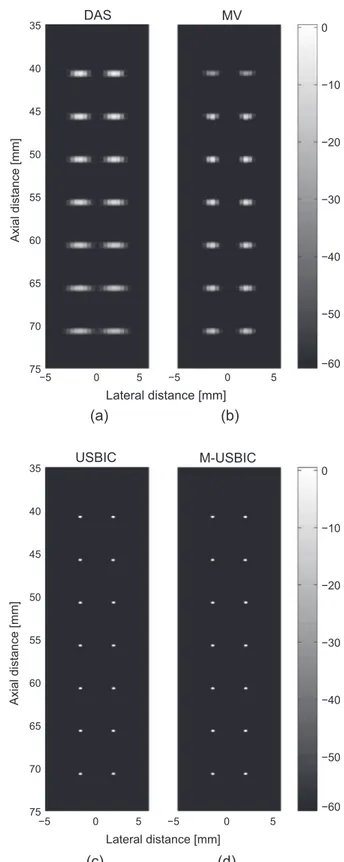
mediums. The results prove that all the 14 sparsely located reflec-tors are detected at correct positions. The beamformed responses
are illustrated inFig. 1. One can observe that using DAS BF with
a Hanning apodisation window (Fig. 1(a)) produces results with
poor lateral resolution and high sidelobes. Although MV offers
bet-ter resolution, the sidelobes are still remarkable,Fig. 1(b). Clearly,
Fig. 1(c) and (d) present superiority over DAS and MV BF in terms of lowering the sidelobes of the final image. These results validate that USBIC and M-USBIC beamformers correctly detect the strong reflectors in a sparse medium. For a sparse medium USBIC and M-USBIC give a good approximation of the reflectors’ position. k can range between 0.8 and 1 for a perfect detection of the number of reflectors. Since we are dealing with a sparse medium with no
speckle,
c
was set to 0 for this result.Note that, even if the amplitude of the response of the reflectors
obtained with DAS is decreasing with depth (seeFig. 1(a)), the
pro-posed method is able to detect the 14 reflectors placed at different depths. Contrarily, a simple thresholding method would firstly select the positions corresponding to the sidelobes of the first reflected echoes before selecting the positions corresponding to scatterers at higher depths.
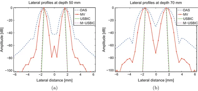
InFig. 2we reinforce the conclusions related to the capability of the strong reflector based approaches to eliminate the sidelobes by drawing the lateral variation of the beamformed responses at axial
depth of 50 mm (Fig. 2(a)) and 70 mm (Fig. 2(b)). We can clearly
observe the ability of USBIC and M-USBIC to correctly detect the isolated scatterers, compared to the relatively large mainlobe and high sidelobes generated by standard beamforming techniques. 5.2. Point reflectors and cyst data
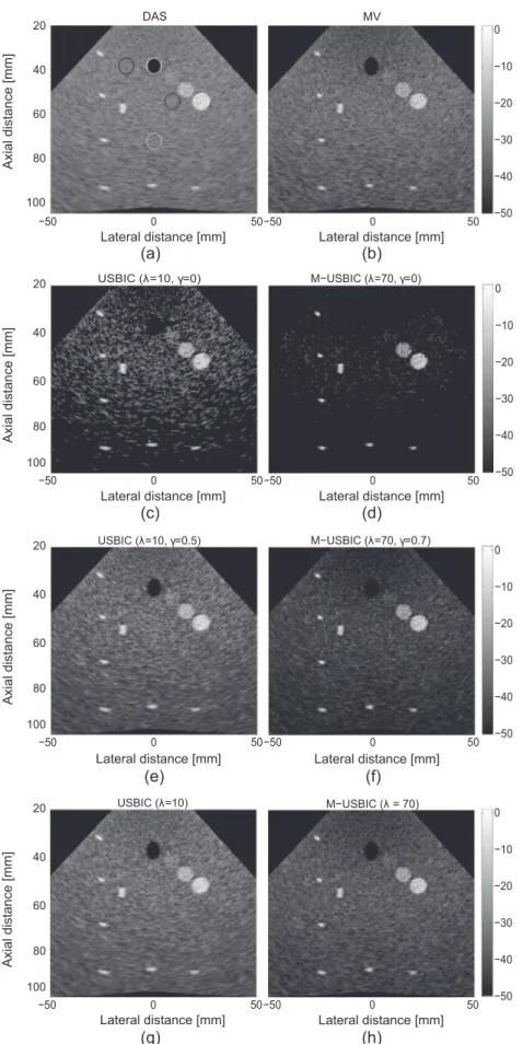
Fig. 3presents the BF results of a simulated medium with the phased array imaging technique. The image quality metrics are
detailed in Table 3. We calculate CR and CNR on anechoic and
hyperechoic cysts (inFig. 3(a), they are delimited by white circles).
For both cases the R2regions are the black circles situated at the
same depth with the bounded cysts, as suggested in[9]. For the
calculation of the SNR, the ROIs are all the black encircled regions together with the gray surrounded region. The SNR was calculated for each region and the final value is the average of the three SNRs.
As stated in[9], while the ROIs of the cysts are chosen exactly at
the limit of the cysts (Fig. 3(a)), we are not greatly enhancing the
contrast by using MV (Fig. 3(b)), compared with DAS. On the other
hand, by using USBIC or M-USBIC BF, it is normal to have a decrease in CR and CNR in comparison with DAS and MV when dealing with the anechoic cyst, since their aim is to remove speckle in the final image. Besides, evaluated for hyperechoic cyst and compared with DAS, M-USBIC has an improvement of more than 10 dB and of 1.6
in CR, respectively CNR,Table 3. With USBIC we can maintain a
good CR even for anechoic cyst, while increasing by more than
10 dB the CR of the hyperechoic cyst,Fig. 3(d). Moreover, the
pro-posed methods provide a trade-off between increasing the contrast and maintaining the speckle in the beamformed images, producing
a gain of 4 in SNR when using M-USBIC BF (Fig. 3(f)) and of 0.7
when using USBIC (Fig. 3(e)), in comparison with DAS. Varying
the parameters k and
c
allows the control of the number of thestrong reflectors and the speckle information in the final image. We need to precise that the results are not too sensitive to the choice of k. A change with an order of 10 must be chosen in order to have some remarkable differences between the final results. However, the higher k is, the more the speckle will be eliminated. This can highly affect the final result, while the speckle contains important information by delimiting the anechoic cyst. As
solu-tions, we can decrease the value of k, or increase the value of
c
, thatrepresents the percentage in the final image of the level of speckle
present in DAS (in the case of USBIC) or MV (in the case of M-USBIC) results. For this example, USBIC BF with k ¼ 10 and
c
¼ 0:5, and M-USBIC BF with k ¼ 70 andc
¼ 0:7 perform the bestresults in terms of preserving the speckle while increasing the contrast of the final image.
(a)
(b)
Axial distance [mm]DAS
MV
−5 0 5 35 40 45 50 55 60 65 70 75 −5 0 5 −50 −40 −30 −20 −10 0 −60 Lateral distance [mm] Axial distance [mm]USBIC
−5 0 5 35 40 45 50 55 60 65 70 75 −5 0 5 −50 −40 −30 −20 −10 0 −60 Lateral distance [mm]M-USBIC
(c)
(d)
Fig. 1. (a) DAS, (b) MV, (c) USBIC, and (d) M-USBIC BF results of 14 sparsely located reflectors.
The main issue of using a low
c
parameter is that the contrast ofanechoic cysts tends to be attenuated with the decrease in
c
. Asimple way to overcome this issue is to choose
c
¼12that is, to give
the weight to each term in(14) and (15)which is a fair (and easy to
achieve) compromise. For example, by adding the images inFig. 3
(a) and (c) we obtain the result inFig. 3(g). Similarly, by summing
the images inFig. 3(b) and (d) results into the image inFig. 3(h).
FromFig. 3(g) and (h) we can observe that the anechoic cyst is bet-ter defined compared with the results when the images obtained
with USBIC and M-USBIC are weighted with
c
. This observation isenforced by the results of CR, CNR and SNR fromTable 3, where
for USBIC (k ¼ 10) the values of CR and CNR for the anechoic cyst are very close to the ones for DAS image, while the SNR is improved. Moreover, the hyperechoic cyst has better contrast than DAS, but not so important as when using the weighting parameter
c
for computing the final result. Similar remarks can be formulatedfor M-USBIC (k ¼ 70) that preserves the low echoic region in the beamformed image. Thus, even if the aim of the proposed methods are to detect the strong reflectors present in the medium, if there exist anechoic structures, they can be preserved, by adding the speckle from the DAS or MV images to the USBIC, respectively
M-USBIC results, without any weighting parameter
c
.The previous observations are enforced byFig. 4, where the
lat-eral profiles around the anechoic (Fig. 4(a)) and hyperechoic (Fig. 4
(b)) cysts are drawn. For this figure we considered USBIC with
k¼ 10 and
c
¼ 0:5 (Fig. 3(e)), and M-USBIC with k ¼ 70 andc
¼ 0:7 (Fig. 3(f)). We can observe that the lateral profile whenusing USBIC is comparable with MV, and has wider mainlobe than
DAS in the case of anychoic cyst’s profile (Fig. 4(a)), while its
pro-pose is to eliminate speckle around the cyst. M-USBIC is eliminat-ing even more the speckle, so the hyperechoic cyst will be enlarged. However, for anechoic cysts M-USBIC provides the
nar-rower mainlobe, the cyst appearing more well defined inFig. 3
(f). The lateral profiles when using USBIC and M-USBIC have lower
average in amplitude, due to the fact that only one fraction ð1 $
c
Þof the DAS and MV beamformed images are added to the image S
(USBIC or M-USBIC), see(14) and (15).
Thus, we may remark that the main advantage of our method is to improve the contrast of hyperechoic structures, based on the detection of strong reflectors. However, by adding speckle to the final images, despite a reduction of this contrast gain, we manage to maintain a contrast of hypoechoic structures close to the one provided by existing beamforming techniques.
For this example, USBIC with k ¼ 10 corresponding to the image inFig. 3(c), required 8783 iterations, that is equivalent to the num-ber of the detected reflectors, while M-USBIC dissociated 1982 strong reflectors, when k ¼ 70 (corresponding to the result in Fig. 3(d)). The two plots corresponding to USBIC and M-USBIC for
this case are drawn inFig. 5. We have also depicted the case when
M-USBIC is used with k ¼ 10, for comparing the impact of keeping the same value of k on the two methods. We can observe that for the same k, M-USBIC tends to detect less strong reflectors (2050), dissociating better than USBIC the strong reflectors from the speckle. This is due to the increase in CR, CNR, and SNR of MV, com-pared with DAS. We also emphasize that the number of strong reflectors detected with M-USBIC only slightly decreases when k changes from 10 to 70.
5.3. Cardiac apical view image
The results of beamforming on a simulated A4C view cardiac
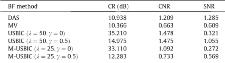
medium are illustrated inFig. 6. To compute CR and CNR, R1was
defined as the region inside the white rectangle around the
posi-tion 58 mm (axial) and $10 mm (lateral) fromFig. 6(a) together
with the R2(the region inside the white rectangle around 8 mm
(axial), situated at the same depth as R1). For SNR, the regions sur-rounded by the black rectangles were chosen. The SNR was
calcu-lated according to(18)for each region and the average value was
extracted.Table 4lists the CR, CNR, and SNR values for each BF
method.
In coherence with the conclusions stated in[9], MV does not
exhibit a higher contrast than DAS when selecting a small ROI, seeTable 4. Contrarily, we obtain an improvement in CR of more than 20 dB with USBIC and M-USBIC, compared with DAS and MV,Fig. 6(c) and (d). Of course, in these situations, due to the elim-ination of the level of speckle, the SNR is much smaller than for DAS and MV. Our empirical experience shows that a value of
k2 50 is optimal in terms of contrast and visual perception of
the resulted beamformed image when we use USBIC BF approach (Fig. 6(e)), and a value of k 2 25 for M-USBIC BF (Fig. 6(f)). When
dealing with a non-sparse medium,
c
is an important parameterthat regulates the appearance of the final image, by controlling
the level of speckle. A value of
c
¼ 0 will result in an image withalmost no speckle,Fig. 6(c) and (d). A small value of
c
is sufficientfor obtaining a trade-off between the contrast enhancement and
retain of speckle information in final image. As
c
increases, theLateral profiles at depth 50 mm
Lateral distance [mm] Amplitude [dB] DAS MV USBIC M−USBIC −6 −4 −2 0 2 4 6 −100 −80 −60 −40 −20 0
(a)
−6 −4 −2 0 2 4 6 −100 −80 −60 −40 −20 0 Amplitude [dB] Lateral distance [mm] Lateral profiles at depth 70 mmDAS MV USBIC M−USBIC
(b)
(a)
(b)
(c)
(d)
(f)
(e)
(g)
(h)
−50 0 50 −50 60 80 100 0 50 −50 0 50 −50 60 80 100 0 50 Lateral distance [mm] Axial distance [mm] 20 40 Lateral distance [mm] M−USBIC (λ=70, γ=0) M−USBIC (λ=70, γ=0.7) −50 0 50 −50 60 80 100 0 50 −50 −40 −30 −20 −10 0 Lateral distance [mm] Axial distance [mm] 20 40 Lateral distance [mm] −50 −40 −30 −20 −10 0 USBIC (λ=10) M−USBIC (λ = 70) −50 −40 −30 −20 −10 0 Lateral distance [mm] Axial distance [mm] 20 40 Lateral distance [mm] Lateral distance [mm] Axial distance [mm] DAS −50 0 50 20 40 60 80 100 −50 0 50 −50 −40 −30 −20 −10 0 MV Lateral distance [mm] USBIC (λ=10, γ=0) USBIC (λ=10, γ=0.5)Fig. 3. Results of (a) DAS, (b) MV, (c) USBIC with k ¼ 10, andc¼ 0, (d) M-USBIC with k ¼ 70 andc¼ 0, (e) USBIC with k ¼ 10; c¼ 0:5, and (f) M-USBIC with k ¼ 70 and c¼ 0:7, (g) USBIC with k ¼ 10, and (h) M-USBIC with k ¼ 70 on a simulated medium using the phased array imaging technique. The image quality metrics: CR, CNR, and SNR are given inTable 3.
contrast of the image is getting closer to the values of DAS, or MV beamformed images. For this simulated medium, the choice of the parameters was influenced on offering continuity of the ventricle structures, while increasing as much as possible the contrast of the final image. USBIC BF achieve the best results with k ¼ 50
and
c
¼ 0:5, while for M-USBIC we obtained the best outcome withk¼ 25 and
c
¼ 0:5.In practical situations, the choice of the hyperparameters k
and
c
may be a difficult task. When dealing with optimizationproblems, the parameter k is usually employed, to balance between the prior information of the strong reflectors and the data fidelity. We may remark that in most of the optimization problems such a hyperparameter is employed. See for example the well-known Least Absolute Shrinkage and Selection Operator
(LASSO) problem[29], where such a parameter balances between
the ‘1 and ‘2norms or algorithms such as Orthogonal Matching
Pursuit (OMP)[30] (similar to our approach in the sense of the
idea of minimizing a ‘0 pseudo norm) where the stop criterion
is either the pre-defined number of atoms or the value of the residuals.
On the other hand, the choice of
c
may depend on theapplica-tion and on the necessity of visualizing the speckle noise in homo-geneous regions or not. Its values are in the range [0, 1], where for 0, no influence of the beamformed data is added to the final result, while for 1 all the speckle information from the beamformed data
is added to the final result.Fig. 7shows how the parameters k and
c
influence the values of CNR and SNR of the beamformed image inthe case of USBIC (Fig. 7(a) and (b)) and M-USBIC (Fig. 7(c) and (d)).
As expected, we can observe that
c
has a great influence on SNR,that is increasing with the value of
c
. This is related to the fact thatTable 3
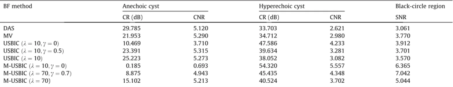
CR, CNR and SNR values of the beamformed images using the simulated point reflectors and cyst data medium,Fig. 3.
BF method Anechoic cyst Hyperechoic cyst Black-circle region
CR (dB) CNR CR (dB) CNR SNR DAS 29.785 5.120 33.703 2.621 3.061 MV 21.953 5.290 34.712 2.980 3.770 USBIC ðk ¼ 10;c¼ 0Þ 10.469 3.710 47.586 4.233 3.912 USBIC ðk ¼ 10;c¼ 0:5Þ 23.391 5.315 39.634 3.281 3.701 USBIC ðk ¼ 10Þ 25.223 5.273 38.052 3.082 3.570 M-USBIC ðk ¼ 10;c¼ 0Þ 0.185 0.693 54.320 5.557 6.365 M-USBIC ðk ¼ 70;c¼ 0:7Þ 8.875 4.943 45.435 4.348 7.042 M-USBIC ðk ¼ 70) 15.102 5.213 40.524 3.702 5.044 −20 −12 −3 5 13 21 −90 −80 −70 −60 −50 −40 −30 Lateral distance [mm] Amplitude [dB] DAS MV USBIC M−USBIC
(a)
13 21 30 38 46 −70 −60 −50 −40 −30 −20 −10 Lateral distance [mm] Amplitude [dB] DAS MV USBIC M−USBIC(b)
Fig. 4. Lateral profiles of the images fromFig. 3. (a) The lateral profile at the axial depth of 40 mm, that intersects the anechoic cyst. (b) The lateral profile at the axial depth of 70 mm, that intersects the hyperchoic cyst. The lateral profiles were drawn considering USBIC with k ¼ 10 andc¼ 0:5 (Fig. 3(e)), and M-USBIC with k ¼ 70 andc¼ 0:7 (Fig. 3(f)). 0 2000 4000 6000 8000 10000 −3000 −2000 −1000 0 1000 2000 K (number of iterations) BIC
USBIC (λ =10)
M−USBIC (λ = 70)
M−USBIC (λ = 10)
K
min=1982
K
min=2050
K
min=8873
Fig. 5. Values of BIC versus K for USBIC with k ¼ 10 andc¼ 0 (Fig. 3(c)) and M-USBIC with k ¼ 70 andc¼ 0 (Fig. 3(d)).
c
is influencing the level of speckle in the final image, by adding to the USBIC or M-USBIC beamformed image a percentage of the DASor MV beamformed image, as discussed in Section3.3. One can
observe that the value of speckle is on one hand influenced by
the l2-norm data fidelity term and on the other hand, by the
hyper-parameters k and
c
. However, the parameter k has further impacton the value of CNR. For example, when applying USBIC BF, a value
of k ¼ 50 and a low
c
results in a maximum of CNR, while for theother values of k, the CNR degrades, seeFig. 7(a). This is not true
in the case of M-USBIC, where the influence of
c
is more importantthat the one of k,Fig. 7(c). This is due to initial decrease of the level
of speckle when applying MV BF.
DAS −20 0 20 20 40 60 80 100 120 Axial distance [mm] MV −20 0 20 −20 0 20 −20 0 20 20 40 60 80 100 120 −50 −40 −30 −20 −10 0 −60
(a)
(b)
(e)
(d)
Lateral distance [mm] Lateral distance [mm] −20 0 20(c)
−50 −40 −30 −20 −10 0 −60 −20 0 20(f)
USBIC (λ=50, γ=0) M−USBIC (λ=25, γ=0) USBIC (λ=50, γ=0.5) M−USBIC (λ=25, γ=0.5) Axial distance [mm]Fig. 6. Results of (a) DAS, (b) MV, (c) USBIC with k ¼ 50, andc¼ 0, (d) M-USBIC with k ¼ 25 andc¼ 0, (e) USBIC with k ¼ 50, andc¼ 0:5, and (f) M-USBIC with k ¼ 25 and c¼ 0:5 on a simulated cardiac apical view image. The image quality metrics: CR, CNR, and SNR are given inTable 4. In (a) we marked the regions used for the calculation of CR, CNR, and SNR.
5.4. Recorded experimental data
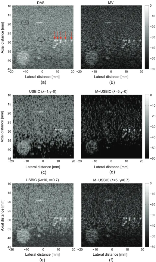
Applied on experimental data, the results of the aforementioned
BF methods are illustrated inFig. 8. To calculate CR and CNR, R1is
represented in the region surrounded by the white ellipse inFig. 8
(a) and R2is inside the black ellipse situated at the same depth as
R1. The three black ellipses fromFig. 8(a) indicate the regions used
to calculate the SNR. For each ellipse its corresponding SNR is cal-culated, the final SNR value being calculated as the average of the three values of SNR. The values of CNR and SNR for this example
are resumed inTable 5. Indeed, the small contrast improvement
(of 0.1 dB, compared with DAS) in the case of MV may be due to
the gain in resolution as stated in[9], the level of speckle,
mea-sured by SNR, decrease. On the other hand, when using MV BF (Fig. 8(b)) the point-like structures are much well defined. We can observe that the tendency of the proposed method on the experimental data is to eliminate the speckle from higher depths, (Fig. 8(c) and (d)). As consequence, we need a relatively high value
of
c
in order to ensure continuity in the final image (c
¼ 0:7), as inFig. 8(e) and (f). Moreover, by increasing k we can achieve better SNR while preserving a good contrast. In the case of USBIC, the beamformed image with the best trade-off between contrast and Table 4
CR, CNR and SNR values of the beamformed images using the simulated cardiac apical view medium,Fig. 6.
BF method CR (dB) CNR SNR DAS 10.938 1.209 1.285 MV 10.366 0.663 0.609 USBIC ðk ¼ 50;c¼ 0Þ 35.210 1.478 0.321 USBIC ðk ¼ 50;c¼ 0:5Þ 14.975 1.475 1.055 M-USBIC ðk ¼ 25;c¼ 0Þ 33.110 1.092 0.272 M-USBIC ðk ¼ 25;c¼ 0:5Þ 12.283 0.733 0.569 0 20 40 60 80 0 0.2 0.4 0.6 0.8 1 0.8 1 1.2 1.4 1.6 1.8 2 2.2 λ γ
Variation of CNR versus λ and γ
0 20 40 60 80 0 0.2 0.4 0.6 0.8 1 0.2 0.4 0.6 0.8 1 1.2 1.4 1.6 λ γ SNR
Variation of SNR versus λ and γ
(a)
(b)
0 10 20 30 40 0 0.2 0.4 0.6 0.8 1 0.7 0.8 0.9 1 1.1 1.2 1.3 1.4 λ γ CNRVariation of CNR versus λ and γ
CNR 0 10 20 30 40 0 0.2 0.4 0.6 0.8 1 0.2 0.4 0.6 0.8 1 1.2 1.4 1.6
λ
γ
SNRVariation of SNR versus λ and γ
(c)
(d)
Fig. 7. The variation of the CNR and SNR versus the parameters k andcwhen USBIC BF method (a and b), and M-USBIC BF method (c and d) are applied to the cardiac view simulation detailed in Section4.3.
speckle preservation was obtained with k ¼ 10 and
c
¼ 0:7, whileM-USBIC performed better when k ¼ 5 and
c
¼ 0:7.For enforcing the previous observations, the lateral profiles are
provided inFig. 9. We considered the case of USBIC with k ¼ 10 and
c
¼ 0:7 (Fig. 8(e)), and of M-USBIC with k ¼ 5 andc
¼ 0:7 (Fig. 8(f)).In the case of the lateral profile that intersects the point-like
reflec-tors,Fig. 9(a), we can observe that for MV and M-USBIC the
scatter-ers are well separated, M-USBIC eliminating as much as possible MV −20 −10 0 10 20 −60 −50 −40 −30 −20 −10 0 Lateral distance [mm] Axial distance [mm] −20 −10 0 10 20 10 15 20 25 30 35 40 45 Lateral distance [mm] Axial distance [mm] −20 −10 0 10 20 10 15 20 25 30 35 40 45 DAS Lateral distance [mm] Lateral distance [mm] M−USBIC (λ=5, γ=0.7) −20 −10 0 10 20 −60 −50 −40 −30 −20 −10 0 USBIC (λ=10, γ=0.7)
(a)
(b)
(c)
(d)
Lateral distance [mm] −20 −10 0 10 20 M−USBIC (λ=5,γ=0) −60 −50 −40 −30 −20 −10 0 Lateral distance [mm] Axial distance [mm] λ γ USBIC ( =1, =0) −20 −10 0 10 20 10 15 20 25 30 35 40 45(f)
(e)
Fig. 8. Results of (a) DAS, (b) MV, (c) USBIC with k ¼ 1, andc¼ 0, (d) M-USBIC with k ¼ 5 andc¼ 0, (e) USBIC with k ¼ 10, andc¼ 0:7, and (f) M-USBIC with k ¼ 5 andc¼ 0:7 on recorded experimental data. The image quality metrics: CR, CNR and SNR are given inTable 5. In (a) we marked the regions used for the calculation of CR, CNR and SNR.
the speckle around them. By using the proposed BF method it is possible to distinguish five point-reflectors (indicated by red arrows), while this is less evident in the case of DAS and USBIC. InFig. 9(b), the profile related to the massive cyst is more narrow than for DAS, MV and USBIC, so just the strongest reflectors inside the cyst are kept.
Even if we are able to highly improve the contrast of the final image by reinforcing the strong reflectors, the main advantage of DAS and MV over USBIC and M-USBIC is the computational time in the case when the scanned medium is not sparse, since the num-ber of the iterations of the proposed methods increases directly with the number of the strong reflectors inside the medium. For
example, to obtain the beamformed images fromFig. 1, we directly
applied the 2D refinement process (USBIC) to the beamformed DAS
image, as described in Section3.2.2, and we obtained a
computa-tional time roughly two times lower than MV BF. The obtained
val-ues are given inTable 6. However, when more complex mediums
are scanned, the 1D initialization process, that is detecting the strong reflectors RF line by RF line, needs to be added to speed up the 2D refinement step. The 1D initialization, described in Sec-tion3.2.1, can be even 10 times longer than MV. However, since it is processed line by line, standard parallel computing methods could highly reduce the computational complexity. The 2D refine-ment method is comparable in time of computation with the MV BF. The computational time values for obtaining the beamformed
images fromFig. 8are given inTable 6, for the case of USBIC
beam-former, and are obtained without using any parallel computing. All the discussed methods were implemented with Matlab R2013b, on an Intel i7 2600 CPU working at 3.40 GHz.
6. Conclusions
In this paper we proposed a beamforming approach based on the detection of the strong reflectors in US imaging. We validate the precision of the detection of the number and the position of the reflectors in a sparse medium, and we evaluate the proposed methods (USBIC and M-USBIC) on different types of simulated data and on experimental data. For a less sparse medium, the k param-eter is deciding the sparsity level in the final beamformed image. Our empirical experience suggests that it can be set between large intervals in a non-sparse medium. For example, by increasing the value of k by a factor of 5, we favor the sparsity in the resulted image. After deciding the best k in function of the desired
experi-ment, the other parameter,
c
will set the level the speckle in thefinal image. For non-sparse mediums, a value of
c
in the interval0.5–0.8 offers the most coherent results, while enhancing the detected reflectors in the final image. Hence, the strong reflector based BF methods allow region differentiation (for example blood vessels, or cysts), while preserving speckle statistics that often con-tain important clinical information. The main disadvantage of the proposed methods is the high computational cost when dealing with highly non-sparse scanning mediums. We should remark that the most computational expensive step is the 1D detection of the strong reflectors. However, this step may be largely fasten by par-allelly processing the RF lines. The automatic choice of the hyper-parameters such as the one balancing between the data fidelity term and the sparsity of the strong reflectors, based for example
on existing cross-validation techniques such as[24,25], is also a
very interesting research track. Finally, the proposed approach may be improved by the use of sparse prior in appropriate bases, other than the direct strong reflection domain.
Table 5
CR, CNR and SNR values of the beamformed images by using the recorded experimental data,Fig. 8.
BF method CR (dB) CNR SNR DAS 3.532 1.602 9.745 MV 3.641 1.085 6.443 USBIC ðk ¼ 1;c¼ 0Þ 6.448 1.943 7.258 USBIC ðk ¼ 10;c¼ 0:7Þ 5.034 1.952 8.702 M-USBIC ðk ¼ 5;c¼ 0Þ 4.013 1 5.408 M-USBIC ðk ¼ 5;c¼ 0:7Þ 4.105 1.745 9.434 5 10 15 20 −60 −50 −40 −30 −20 −10 Lateral distance [mm] DAS MV USBIC M−USBIC Amplitude [dB]
(a)
−60 Lateral distance [mm] USBIC M−USBIC Amplitude [dB] −18 −16 −14 −12 −10 −8 −6 −4 −50 −40 −30 −20 −10 DAS MV USBIC M−USBIC(b)
Fig. 9. Lateral profiles of the images fromFig. 8. (a) The lateral profile at the axial depth of 28 mm, that intersects the point reflectors. The red arrows correspond to the point-like reflectors indicated inFig. 8(a) by red arrows. (b) The lateral profile at the axial depth of 40 mm, that intersects the massive cyst. We considered the case of USBIC with k¼ 10 andc¼ 0:7 (Fig. 8(e)), and of M-USBIC with k ¼ 5 andc¼ 0:7 (Fig. 8(f)). (For interpretation of the references to color in this figure legend, the reader is referred to the web version of this article.)
Table 6
Computational time required to beamform the images inFigs. 1 and 8. BF method Computational time (min)
Fig. 1 Fig. 8
DAS 0.075 0.215
MV 5.124 10.272
1D initialization – 72.763
Acknowledgements
We wish to thank Adeline Bernard and Hervé Liebgott, from CREATIS laboratory, University of Lyon, for providing the experimental ultrasound phantom data. This work was partially supported by ANR-11-LABX-0040-CIMI within the program ANR-11-IDEX-0002-02 of the University of Toulouse.
References
[1] B.D. Van Veen, K.M. Buckley, Beamforming: a versatile approach to spatial filtering, IEEE ASSP Mag. 5 (2) (1988) 4–24.
[2] J. Capon, High-resolution frequency-wavenumber spectrum analysis, Proc. IEEE 57 (8) (1969) 1408–1418.
[3] K.L. Bell, Y. Ephraim, H.L. Van Trees, A bayesian approach to robust adaptive beamforming, IEEE Trans. Signal Process. 48 (2) (2000) 386–398.
[4] J. Li, P. Stoica, Z. Wang, On robust capon beamforming and diagonal loading, IEEE Trans. Signal Process. 51 (7) (2003) 1702–1715.
[5] B.M. Asl, A. Mahloojifar, A low-complexity adaptive beamformer for ultrasound imaging using structured covariance matrix, IEEE Trans. Ultrason. Ferroelectr. Freq. Control 59 (4) (2012) 660–667.
[6] B.M. Asl, A. Mahloojifar, Minimum variance beamforming combined with adaptive coherence weighting applied to medical ultrasound imaging, IEEE Trans. Ultrason. Ferroelectr. Freq. Control 56 (9) (2009) 1923–1931. [7] I.K. Holfort, F. Gran, J.A. Jensen, Broadband minimum variance beamforming
for ultrasound imaging, IEEE Trans. Ultrason. Ferroelectr. Freq. Control 56 (2) (2009) 314–325.
[8] K. Diamantis, I.K. Holfort-Voxen, A.H. Greenaway, T. Anderson, J.A. Jensen, V. Sboros, A comparison between temporal and subband minimum variance adaptive beamforming, in: SPIE Medical Imaging, International Society for Optics and Photonics, 2014, pp. 90400L–90400L.
[9] O.M.H. Rindal, J.P. Asen, S. Holm, A. Austeng, Understanding contrast improvements from capon beamforming, in: Ultrasonics Symposium (IUS), 2014 IEEE International, IEEE, 2014, pp. 1694–1697.
[10] T. Yardibi, J. Li, P. Stoica, Nonparametric and sparse signal representations in array processing via iterative adaptive approaches, in: 42nd Asilomar Conference on Signals, Systems and Computers, 2008, IEEE, 2008, pp. 278–282. [11] T. Yardibi, J. Li, P. Stoica, M. Xue, A.B. Baggeroer, Source localization and sensing: a nonparametric iterative adaptive approach based on weighted least squares, IEEE Trans. Aerosp. Electron. Syst. 46 (1) (2010) 425–443. [12] A.C. Jensen, Austeng, The iterative adaptive approach in medical ultrasound
imaging, IEEE Trans. Ultrason. Ferroelectr. Freq. Control 61 (10) (2014) 1688– 1697.
[13] C. Quinsac, A. Basarab, J. Girault, D. Kouamé, Compressed sensing of ultrasound images: sampling of spatial and frequency domains, in: 2010 IEEE Workshop on Signal Processing Systems (SIPS), IEEE, 2010, pp. 231–236.
[14] R. Tur, Y.C. Eldar, Z. Friedman, Innovation rate sampling of pulse streams with application to ultrasound imaging, IEEE Trans. Signal Process. 59 (4) (2011) 1827–1842.
[15] N. Wagner, Y.C. Eldar, Z. Friedman, Compressed beamforming in ultrasound imaging, IEEE Trans. Signal Process. 60 (9) (2012) 4643–4657.
[16] T. Szasz, A. Basarab, M.-F. Vaida, D. Kouamé, Beamforming with sparse prior in ultrasound medical imaging, in: Ultrasonics Symposium (IUS), 2014 IEEE International, IEEE, 2014, pp. 1077–1080.
[17] J. Li, P. Stoica, Robust Adaptive Beamforming, Wiley Online Library, 2006. [18] J.-F. Synnevag, A. Austeng, S. Holm, Adaptive beamforming applied to medical
ultrasound imaging, IEEE Trans. Ultrason. Ferroelectr. Freq. Control, 54 (8) (2007) 1606–1613.
[19] J.-F. Synnevag, C.-I. Nilsen, S. Holm, P2b-13 speckle statistics in adaptive beamforming, in: Ultrasonics Symposium, 2007. IEEE, IEEE, 2007, pp. 1545– 1548.
[20] J.-F. Synnevag, A. Austeng, S. Holm, Benefits of minimum-variance beamforming in medical ultrasound imaging, IEEE Trans. Ultrason. Ferroelectr. Freq. Control 56 (9) (2009) 1868–1879.
[21] S. Konishi, G. Kitagawa, Information Criteria and Statistical Modeling, Springer Science & Business Media, 2008.
[22] E.J. Candes, M.B. Wakin, S.P. Boyd, Enhancing sparsity by reweighted ‘1 minimization, J. Fourier Anal. Appl. 14 (5–6) (2008) 877–905.
[23] N. Dobigeon, A. Basarab, D. Kouamé, J.-Y. Tourneret, Regularized bayesian compressed sensing in ultrasound imaging, in: 2012 Proceedings of the 20th European Signal Processing Conference (EUSIPCO), IEEE, 2012, pp. 2600–2604. [24] N.P. Galatsanos, A.K. Katsaggelos, Methods for choosing the regularization parameter and estimating the noise variance in image restoration and their relation, IEEE Trans. Image Process. 1 (3) (1992) 322–336.
[25] S. Ramani, Z. Liu, J. Rosen, J. Nielsen, J.A. Fessler, Regularization parameter selection for nonlinear iterative image restoration and MRI reconstruction using GCV and SURE-based methods, IEEE Trans. Image Process. 21 (8) (2012) 3659–3672.
[26] J.A. Jensen, N.B. Svendsen, Calculation of pressure fields from arbitrarily shaped, apodized, and excited ultrasound transducers, IEEE Trans. Ultrason. Ferroelectr. Freq. Control 39 (2) (1992) 262–267.
[27] M. Alessandrini, H. Liebgott, D. Friboulet, O. Bernard, Simulation of realistic echocardiographic sequences for ground-truth validation of motion estimation, in: 19th IEEE International Conference on Image Processing (ICIP), 2012, IEEE, 2012, pp. 2329–2332.
[28] M. Xu, X. Yang, M. Ding, M. Yuchi, Spatio-temporally smoothed coherence factor for ultrasound imaging [correspondence], IEEE Trans. Ultrason. Ferroelectr. Freq. Control 61 (1) (2014) 182–190.
[29] R. Tibshirani, Regression shrinkage and selection via the lasso, J. Roy. Stat. Soc. Ser. B (Methodological) (1996) 267–288.
[30] J.A. Tropp, A.C. Gilbert, Signal recovery from random measurements via orthogonal matching pursuit, IEEE Trans. Inf. Theory 53 (12) (2007) 4655– 4666.