Transient effects of squeeze and starvation in an EHL contact under forced oscillation: On the film-forming capability

OATAO is an open access repository that collects the work of Toulouse

researchers and makes it freely available over the web where possible

Any correspondence concerning this service should be sent

to the repository administrator:

tech-oatao@listes-diff.inp-toulouse.fr

This is an author’s version published in: http://oatao.univ-toulouse.fr/25916

To cite this version:

Yahiaoui, Malik

and Mazuyer, Denis and Cayer-Barrioz, Juliette

Transient effects of squeeze and starvation in an EHL contact under

forced oscillation: On the film-forming capability. (2020) Tribology

International, 150. 106375. ISSN 0301-679X

Official URL:

https://doi.org/10.1016/j.triboint.2020.106375

Transient effects of squeeze and starvation in an EHL contact under forced

oscillation: On the film-forming capability

M. Yahiaoui

_{, D. Mazuyer}

_{, J. Cayer-Barrioz}

a_{Laboratoire de Tribologie et Dynamique des Systèmes, École Centrale de Lyon, CNRS UMR5513, 36 avenue Guy de Collongue, 69130 Écully, France} b_{Laboratoire Génie de Production, Université de Toulouse, Ecole Nationale d’Ingénieurs de Tarbes, 47 avenue d’Azereix, 65000 Tarbes, France}

A R T I C L E I N F O

A B S T R A C T

This study provides a new insight on the EHL regime in time-varying conditions. A full-analytical resolution of the Reynolds equation was proposed considering forced oscillations. Confronted to experimental validation, the analytical film thickness equations provide perfect modeling of the film forming mechanisms: squeeze induced by the transient evolution of the film thickness with time, asymmetry and hysteresis in the film distribution resulting from the change in direction and the transport effect. Furthermore, the analytical equations combined with a modulation of the inlet flow give an accurate prediction of the effects induced by the starvation resulting from the change in direction, i.e. as the original outlet zone becomes the next inlet zone.

1. Introduction

Various dynamic phenomena can induce a perturbation in the film-forming capability of a lubricated contact such as the surface rough-ness, the heterogeneity of the confined lubricant, the presence of a boundary film on the surfaces, the time-varying tribological conditions (load or velocity), or the transient changes in the flooding regimes. For example, the local increase in lubricant film thickness observed with laser-textured surfaces is mainly related to the squeeze-term of the Reynolds equation that cannot be neglected even when the velocities are stationary (see [1–3]).

In colloidal lubrication, shearing of complex fluids in confined interfaces submitted to reciprocating motions promoted film instabili-ties [4–7], which were correlated with local friction variations. Similar observations were also made for more simple fluids within time-varying conditions and were qualitatively backed-up by numerical (more or less simplified) resolution of Reynolds equation (see [8–15]). Compared to the classical steady-state film thickness prediction by Hamrock–Dowson or Moes–Venner models [16,17], the numerical solutions of the full Reynolds equation including the transient term capture features such as the hysteretic nature of the film thickness evolution or successive squeeze [15]. The effects of the velocity or the deceleration rate has been investigated experimentally and theoretically in [18] and in [19], respectively. A tentative general theoretical solution of the Reynolds equation for non-stationary elastohydrodynamic was proposed by [20]. Nevertheless, this approximated solution was in parametric form using the velocity as a parameter, making the application of this solution

difficult for transient conditions. The first successful analytical solution of the full Reynolds equation in 1D and 2D can be found in [19] for linear deceleration. This solution was experimentally validated over two decades of viscosity in the range of deceleration between 0.004 and 0.2 m/s2_{under fully-flooded conditions. It is worth noting}

that all these works concerns fully-flooded contacts. However when lubricated contacts are submitted to reciprocating motions, the oil-supply conditions may change during time: for instance, the contact becomes transitorily starved at the position where the direction of the displacement changes (see figure 8 in [21]). The starvation phenomena are referred in the literature only under steady-state kinematics either experimentally [22–25] or numerically [26–28]. For smooth contacts, the starvation mechanisms resulted from the balance between the flow rates, in the inlet zone, : a competition between Poiseuille and Couette flows leads to the formation of a small reservoir at the entrance of the Hertz contact. Along the transverse direction (i.e. perpendicular to the entrainment velocity direction), only the Poseuille flow is responsible for the ejection of the fluid while in the outlet, the fluid is ejected in the direction of the flow and entrained away from the contact. A dimensionless master curve was obtained by [26] to define the transition between starved and fully-flooded regime in steady-state conditions. This transition was governed by a parameter, function of the two Moes parameters M and L.

In this framework, the film-forming mechanisms in a smooth EHL contact moved by forced oscillating velocities (succession of accelera-tion/deceleration cycles) were analyzed considering the contributions ∗ Corresponding author at: Laboratoire Génie de Production, Université de Toulouse, Ecole Nationale d’Ingénieurs de Tarbes, 47 avenue d’Azereix, 65000 Tarbes, France.

Nomenclature

𝛿 Stroke distance, m;

𝜂 Lubricant viscosity, Pa s;

𝛾 Reduction factor exponent;

𝜎 Dimensionless space–time parameter;

𝜏 Acceleration or deceleration time, s;

𝜉 Non-null sign function;

𝑏 Hertzian radius, m;

ℎ Film thickness, m;

ℎc Hamrock–Dowson film thickness, m;

𝐻 Dimensionless film thickness;

𝐻_2𝑛, 𝐻_2𝑛+1 Odd and even iterations of film thickness calculation;

𝐿 Moes dimensionless material parameter;

𝑀 Moes dimensionless load parameter;

𝑝 Contact pressure, Pa;

𝑟 Successive iterations film thickness ratio;

𝑅 Ball radius, m;

𝑅∗= ₁2 𝑅a+

1

𝑅a

Combined surface roughness, m;

𝑅a Contact bodies surface roughness, m;

 Reduction factor;

𝑆, 𝑆∗ Dimensionless space–time parameter;

𝑡 Time, s;

𝑇 Dimensionless time;

𝑢 Entrainment velocity, m/s;

𝑢1, 𝑢2 Absolute velocities of contact bodies, m/s;

𝑢_max Maximum velocity, m/s;

𝑥 Position in the contact, m;

𝑋 Dimensionless position;

𝑋₁ Convergent position;

𝑋_𝑚 Divergent position;

𝑋_𝑚 Divergent position.

of both squeeze and starvation. Thanks to an extension of a recent theoretical work [19], an analytical solution of Reynolds equation was proposed and experimentally validated to get a better understanding of the lubrication mechanisms under these time-varying conditions. In addition to bring a full prediction of the film thickness, a quan-tification of the starvation degree, was provided by the confrontation analytical/experimental film thickness.

2. Modeling of transient EHL line contact 2.1. General assumptions

The Reynolds equation that models the coupling between the film thickness ℎ(𝑥, 𝑡) and the pressure 𝑝(𝑥, 𝑡) within a lubricated contact between two solids can be written in one dimension as:

𝜕 𝜕𝑥 [ ℎ3 𝜂 𝜕𝑝 𝜕𝑥 ] = 6𝑢(𝑡)𝜕ℎ 𝜕𝑥+ 12 𝜕ℎ 𝜕𝑡 (1)

with 𝑢(𝑡) = 𝑢1(𝑡) + 𝑢2(𝑡)the entrainment velocity, 𝜂 the viscosity of the

fluid under pressure following the Barus law (taken for mathematical convenience), 𝑥 the position in the contact and 𝑡 the time. The general assumptions required to get an analytical solution of the Reynolds equa-tion includes Ertel hypotheses and Crook’s approximaequa-tion. They are detailed in [19]. Then, the Reynolds equation was solved by successive integrations in the contact inlet and in the Hertzian contact consid-ering the fluid entrainment and squeeze contributions. The resulting analytical solution was proposed and experimentally backed-up in the

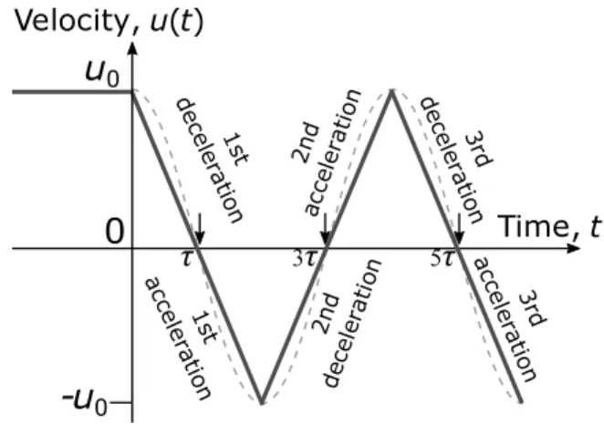
Fig. 1. Triangular velocity profile after an initial constant velocity step. 𝜏 represents the

deceleration/acceleration duration. Each step is described and the change in directions is indicated with an arrow. The associated sine velocity used in reciprocating sliding experiments is superimposed in dashed line.

case of a linear deceleration over a deceleration time 𝜏. We showed that it was mandatory to account for the squeeze contribution and the transport effects in the lubricant flow to predict the evolution of the film thickness according to time and contact position.

Here, a similar approach was used, solving analytically the Reynolds equation in three zones: the convergent, the high-pressure zone and the constriction zone. Accounting for the constriction zone was here compulsory as the outlet zone becomes the new inlet zone at each change in direction. To model the forced oscillations, after an initial step at constant velocity 𝑢0, as a first approximation, the velocity profile

was set triangular instead of sinusoidal as in the reciprocating sliding experiments (Fig. 1). In this case, it is important to emphasize that after a deceleration, when the velocity vanishes, the following acceleration was performed with a change of direction. Nevertheless, after the acceleration, the deceleration takes place in the same direction. In the remainder of the paper, the deceleration phase (resp. acceleration phase) corresponds to a decrease in|𝑢(𝑡)| (resp. an increase in |𝑢(𝑡)|).

In the central contact zone, the pressure field was assumed constant. The Reynolds equation (Eq.(1)) was simplified as follows:

𝑢(𝑡)𝜕ℎ 𝜕𝑥+ 2

𝜕ℎ

𝜕𝑡 = 0 (2)

This equation can then be solved using the method of character-istics as described in [19]. Consequently, three main film thickness equations can be proposed during the first deceleration, the follow-ing accelerations and decelerations based on the work of Mazuyer et al. [19].

2.2. Film thickness equations

First of all, the following dimensionless parameters were calculated from the distance 𝑥, the time 𝑡 and the film thickness ℎ:

• The dimensionless distance 𝑋 = 𝑥_𝑏 with 𝑏 the Hertzian radius. Then, 𝑋₁corresponds to the dimensionless position at the end of the inlet and 𝑋mto the one at the beginning of the outlet.

• The dimensionless time 𝑇 =𝑡𝑢_𝑏0.

• The dimensionless film thickness 𝐻 =_ℎ(0,0)ℎ(𝑥,𝑡).

• The dimensionless space–time parameters 𝜎 =𝜏𝑢_𝑏0 and 𝑆 = 1 −𝑇_𝜎. The dimensionless contact film thickness during the first deceler-ation 𝐻1(𝑋, 𝑆)can be expressed by the equations system(3). 𝑆 = 1

corresponds to 𝑡 = 0 and then 𝐻₀[𝑋] = 𝐻[𝑋, 𝑆 = 1]corresponds to the initial thickness profile (i.e. in pure rolling before the first decel-eration). This initial film thickness can be measured with a constant

velocity experiment or generated using Hamrock–Dowson equation and Crook’s approximation or generated with a numerical simulation [29]. ⎧ ⎪ ⎪ ⎪ ⎪ ⎨ ⎪ ⎪ ⎪ ⎪ ⎩ if 𝑋 ≥ 𝑋₁+𝜎 2(1 − 𝑆 2₎ 𝐻1(𝑋, 𝑆) = 𝐻0(𝑋) else 𝐻₁(𝑋, 𝑆) = 𝐻₀(𝑋) ⋅ e− 𝜎 4 ⋅𝑆∗2 [ e−𝜎3+√𝜎𝜋 3 [ erf(√𝜎 3 ) −erf(√𝜎 3⋅𝑆∗ )]]3∕4 with, if 𝑋 < 𝑋1, 𝑆∗= 𝑆else 𝑆∗= √ 𝑆2₊2(𝑋−𝑋1) 𝜎 (3)

During the accelerations, with an initial change in direction, the dimensionless film thickness 𝐻2, 𝐻4,… , 𝐻2n(∀𝑛 ∈ N∗) are defined by

the equations systems(4)and(5). Using, 𝛷(𝑋, 𝑆∗_{) = 𝐻} 0(𝑋) ⋅ e 𝜎 4 ⋅𝑆∗2 [( 𝐻0(𝑋) 𝐻2n−1(−𝜉⋅𝑋m) )4∕3 −√𝜎𝜋 3erfi (√𝜎 3⋅𝑆∗ )]3∕4 and the

non-null sign function 𝜉 = { 1if 𝑆 ≥ 0 −1if 𝑆 < 0. ∀𝑋 ∈ [−𝑋_m, 𝑋_m] ⎧ ⎪ ⎪ ⎨ ⎪ ⎪ ⎩ if 𝑋 ≥ −𝑋m+𝜎₂𝑆2 𝐻_2n(−𝑋, 𝑆) = 𝐻2n−1 [ 𝜉 ⋅ (𝑋 −𝜎₂𝑆2₎] else 𝐻_2n(−𝑋, 𝑆) = 𝛷(𝑋, 𝑆∗_{)with 𝑆}∗_{= −}√_𝑆2₋2(𝑋m+𝑋) 𝜎 (4) ∀𝑋 ∉ [−𝑋m, 𝑋m] × ⎧ ⎪ ⎪ ⎪ ⎪ ⎨ ⎪ ⎪ ⎪ ⎪ ⎩ if 𝑋 < −𝑋m, 𝐻2n(−𝑋, 𝑆) = 𝛷(−𝑋m, 𝑆∗)with 𝑆∗= −|𝑆| ⎧ ⎪ ⎪ ⎪ ⎨ ⎪ ⎪ ⎪ ⎩ if 𝑋 > 𝑋mand|𝑆| > 1 2, 𝐻2n(−𝑋, 𝑆) = 𝛷(−𝑋m, 𝑆∗) with 𝑆∗_{= −}√_𝑆2₋4𝑋m 𝜎 , if|𝑆| ≥ 4𝑋m 𝜎 else 𝑆∗_{= −}√_𝑆2_{− 𝜉 ⋅}2(𝑋1+𝑋) 𝜎 else 𝐻_2n(−𝑋, 𝑆) = 𝐻2n−1[𝜉 ⋅ 𝑋] (5)

During the following decelerations (i.e. except the initial one), the dimensionless film thickness 𝐻₃,… , 𝐻_2n+1(∀𝑛 ∈ N)are defined by the Eq.(6). 𝐻_{2n+1(𝜉 ⋅ 𝑋, 𝑆) = 𝐻0}(𝑋) ⋅ e −𝜎 4⋅𝑆 ∗2 [( 𝐻0(−𝑋m) 𝐻2n(𝑋1) )4∕3 +√𝜎𝜋 3 [ erf(√𝜎 3 ) −erf(√𝜎 3⋅ 𝑆 ∗)]] 3∕4 (6)

with, if 𝑋 < 𝑋1 and 𝑋 < 𝑋1 + 𝜎₂(1 − 𝑆2), 𝑆∗ = |𝑆| else 𝑆∗ =

√

𝑆2₊2(𝑋−𝑋1)

𝜎 .

2.3. Film thickness evolution with position and time

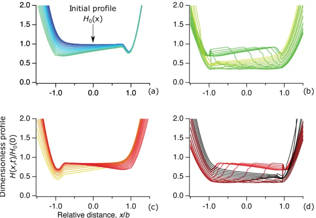
The evolution of the film thickness profile as a function of time and position is presented inFig. 2. In addition, the waterfall representation inFig. 3a gives this evolution in a single view. It is noteworthy that the transient effects are well described here as the hysteresis between the deceleration and acceleration periods is well highlighted. After the first cycle, the film thickness decreased to reach a steady-state level and the evolution of the film thickness was then identical in the following cycles.

In more detail, it can be seen that:

• The initial profile, 𝐻0(𝑋), corresponds to the profile at constant

velocity with a fluid flow going from the left to the right. • Then, during the first deceleration, as the velocity decreases,

the film thickness decreases from the inlet and this decrease propagates to the rest of the contact with time. However, at zero velocity, the surfaces are still rather well separated, consistently with [19].

• During the first acceleration, the change of sliding direction pro-duces lower film thickness of lubricant in relation with the prop-agation of the dimple formed at zero velocity and of the thin film constriction zone. This clearly illustrates the transport effect taking place in the contact. After this phase, the film thickness starts increasing again.

• During the second deceleration, the film thickness keeps increas-ing and reaches its maximum amplitude (however, the amplitude of the initial profile is not retrieved here). Then, the profile amplitude slightly decreases until a local minimum.

• During the second acceleration, again, with the change in direc-tion, the dimple formed at zero velocity propagates through the contact and the film thickness decreases before starting increas-ing.

The plot of the central film thickness confirms these observations (seeFig. 3b). This analytical model predicts the evolution of the film thickness in fully-flooded conditions. The asymmetry in film thickness distribution during acceleration and deceleration phases results in a strong hysteresis in the film thickness.

3. Experimental validation 3.1. Device setup

The experiments were performed using a forced oscillations tri-bometer CHRONOS described in [21]. The contact is in ball-on-flat configuration using a fixed steel ball with a diameter of 25.4 mm and a quartz moving flat counterpart. The flat quartz counterpart has a semi-reflective coating to allow optical measurement of lubricant film thickness distribution. Before the experiments, the ball was approached to the counterpart and a drop of polyalphaolefin (PAO) was set between the two surfaces to form a meniscus. Then, the sinusoidal movement was launched without contact to avoid wear at the beginning of the strokes. Once the motion set, a constant normal load was applied and the contact was formed and visualized. The experimental measurement began after tens of sliding cycles and the first cycles were not acquired. The following contact conditions were used in this study for the experimental validation and the calculation:

• The steel ball Young modulus is of 210 GPa and the Poisson ratio is of 0.3. The glass flat has a Young modulus of 70 GPa and a Poisson ratio of 0.17.

• The surface roughness of both sphere and flat measured at 𝑅a=

14 ± 1 nmgive then a combined surface roughness 𝑅∗_{= 14 ± 1 nm.}

• A lubricant drop of 20 μL of a PolyAlphaOlefin oil at a room temperature of 20.5◦_{C with a corresponding viscosity of 0.8 Pa}

s.

• A load fixed at 5, 10, 15 or 20 N corresponding to respective Hertzian contact pressures of 175, 220, 252 or 278 MPa and contact radius 𝑏 of 95, 120, 137 and 151 μm. The nominal load was 10 N.

• The nominal stroke length 𝛿 was fixed at 1 mm which is at least six times larger than the contact radius.

• The nominal frequency was fixed at 10 Hz.

• Observations were performed using a speed camera with a frame size of 1600 × 500 pixel2_{, a resolution of 1.6 μm/pixel and a frame}

rate of 1000 fps. This camera is associated with a lens allowing interferometric measurements [21].

In these conditions, neither wear nor roughness modification was detected after the experiments. However, the first steps of the velocity profiles (pure rolling and first cycles) were missed.

Fig. 2. Evolution of the dimensionless film thickness profile as a function of time and position: (a) first deceleration from pure rolling phase i.e. the initial film thickness (from

blue to green); (b) change in direction and first acceleration (from green to yellow); (c) second deceleration (from yellow to red); (d) change in direction and second acceleration (from red to black). (For interpretation of the references to colour in this figure legend, the reader is referred to the web version of this article.)

Fig. 3. Evolution of the dimensionless film thickness with dimensionless time during the first two cycles: (a) waterfall display of film thickness distribution; (b) central film

thickness.

3.2. Contact visualization under forced oscillations

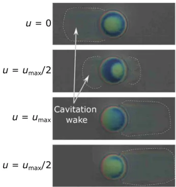
The lubricated interface displays similar periodic dynamics as shown inFig. 4:

• After deceleration, at zero velocity, the interface shows a typical circular zone of squeezed entrapped lubricant surrounded by a ring constriction zone.

• During an acceleration with a change in direction, the previously squeezed lubricant volume flowed out of the contact and a new volume of lubricant flowed in the contact. This step highlights the lubricant transport effect i.e. the transport of the well-identified squeezed lubricant volume in the middle of the contact around 𝑢=0 to the contact outlet around 𝑢 = 𝑢max

2 . The time needed to

performed this transport of lubricant is called the residence time in the rest of this paper.

Fig. 4. Contact interferograms from a zero velocity to half maximum velocity and

maximum velocity during an acceleration and to half maximum velocity during a deceleration (purple ≈ 3 nm, blue ≈ 10 nm, green ≈ 70 nm and red ≈ 140 nm) for 0.8 Pa s at a load of 10 N i.e. a contact radius of 120 μm. (For interpretation of the references to colour in this figure legend, the reader is referred to the web version of this article.)

• Around maximum velocity, the conventional EHL horse-shoe shape appears with a large homogeneous inner zone of equal lubricant thickness.

• During a deceleration, most of the lubricant volume is maintained by the squeeze effect in the contact and a small amount of lubricant flows out of the contact. And so on, the contact is emptied once again during the next acceleration.

Experimentally, a transient starvation effect due to the presence of a smaller fluid volume in the inlet zone, was clearly visible in front of the contact around the maximum velocity. This phenomenon can be explained by the time-varying length and position of the cavitation wake length. At the change in direction, the original exit zone becomes the inlet zone and a smaller lubricant reservoir flows in the contact leading to a starvation effect.

3.3. Film thickness measurement

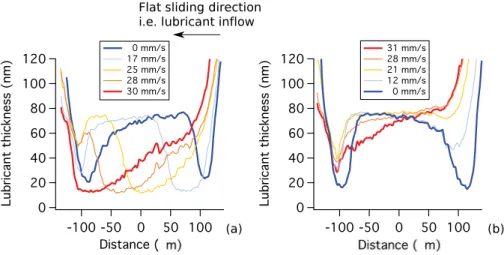
The central longitudinal profiles of lubricant film thickness can be plotted to give a clear view of the lubricant dynamic during an acceleration and a deceleration (Fig. 5) for the reference conditions:

• At zero velocity, the squeezed lubricant is confined to form a dim-ple of a maximum film thickness around 70 nm and surrounded by a ring of constriction of thickness around 20 nm.

• During the following acceleration (Fig. 5a), the confined dimple flows towards the exit constriction. Then, as this fluid volume flows out of the contact, a new volume of lubricant simulta-neously enters the contact front (e.g. here after a velocity of 20 mm/s). Around the maximum velocity, the squeeze volume is totally out of the contact. The profile forms a wedge.

• During the deceleration (Fig. 5b), from the wedge shape, the profile tends towards the EHL classical horse-shoe shape profile observed in the constant velocity experiments. When approaching the zero velocity, the profile forms again the shape of a dimple.

These observations remain valid for the whole range of contact size and pressure investigated. As predicted by the calculation (see Fig. 2), the lubricant film thickness never reaches zero even when the velocity is null. For instance, with a viscosity of 0.8 Pa s, at 10 Hz and under a load of 10 N, the minimum film thickness is about 14 nm. In addition, the evolution of the film thickness presented inFig. 2and5 are identical.

4. Film thickness mechanisms and discussion 4.1. Transient squeeze & residence time effect

For the first deceleration, the theoretical calculation was perfectly well backed-up in [19] for 70 different experimental conditions. In the present work, when the initial deceleration is followed by a change in direction and acceleration, for reference conditions, at 10 Hz and for a viscosity of 0.8 Pa s, the comparison inFig. 6between the dimen-sionless experimental and theoretical central film thickness evolutions also shows a very good agreement. Both shapes follow the same trend and are very similar, confirming that the main mechanisms, here the transient squeeze and the transport effect, are well accounted for by the theory. In addition, it is also interesting to note that between an acceler-ation and a deceleracceler-ation the measured thickness displayed an inflection not predicted by the calculated film thickness (see Section4.2).

The contact size 𝑏 and the stroke distance 𝛿 have a direct influence on the transient squeeze and the transport effect, even though the mechanisms remain identical. These two parameters directly influence the lubricant residence time in the contact. Furthermore, the experi-ments and the calculation showed that neither the sliding frequency nor the viscosity have an effect on the residence time. In this way, the dimensionless time parameter 𝜎 = 𝜏𝑢0

𝑏 = 𝜋 4 ⋅

𝛿

𝑏 highlighted by the

analytical resolution combines the contact size and the stroke distance. In other word, the larger the contact size or the smaller displacement amplitude, the longer the lubricant flow residence time. At low 𝜎 values, i.e. at relatively high contact load/large contact size (here at constant displacement amplitude), the local minimum observed at the zero velocity, when t/T = 0.25 and 0.75, disappears (Fig. 6a) which is well predicted by the calculation (Fig. 6b). At high 𝜎 value, i.e. here at smaller contact size, a larger drop of film thickness around the zero velocity was then observed. This seems to confirm the role played by the residence time in the observation of the film drop. A detailed investigation of the effects of the displacement amplitude could validate this interpretation in the future. Eventually, it is also clear that the dimensionless film thickness level and spread between 0.3 and 0.8 was not affected by the change of contact load/size.

4.2. Starvation effect consideration

Even though the theoretical calculation well predicts the trends observed experimentally, the level of the central film thickness is over-estimated by the theory. This can be attributed to starvation observed experimentally. It is induced by the change in direction, when the orig-inal outlet becomes the inlet and the contact crosses over the previous and persistent cavitation wake (seeFig. 4). To take in consideration this starvation effect, a film thickness reduction factor  was added in the analytical solution (Eq.(7)). In the previous Eqs.(4), (5)and (6), the initial profile term 𝐻0(𝑋) was modulated by the  factor:

× 𝐻0(𝑋). The first deceleration was obviously not affected by any

starvation effect and no starvation coefficient was applied to the Eq.(3). The film thickness reduction factor was first proposed by Chevalier et al. [30] and associated to a factor 𝛾 for constant velocity conditions. In those conditions, Damiens et al. [31] interpreted the 𝛾 factor as the resistance that the contact opposes to the lubricant which tries to bypass it. Such resistance reduces contact bypass by the lubricant. It therefore forces it to cross the contact. Damiens et al. considered the inlet area could be regarded as a tube in which part of the lubricant

Fig. 5. Longitudinal profiles of lubricant film thickness with a viscosity of 0.8 Pa s, at 10 Hz and under a load of 10 N (i.e. a Hertzian radius of 120 μm): (a) during an acceleration

with inflow from right to left; (b) during a deceleration.

Fig. 6. Dimensionless central lubricant film thickness measurement (a) and calculation (b) with a viscosity of 0.8 Pa s at a sliding frequency of 10 Hz with Hertzian radii from

95 μm to 151 μm.

flow is diverted to the contact periphery. Thus, by modeling the lateral flow of the ejected lubricant in this tube, he showed a linear relation between the 𝛾 factor and the square root of the ratio of Moes dimension-less load parameter M and to Moes dimensiondimension-less material parameter L. This ratio is related to the size of the inlet area which is constant in a steady-state regime. In time-varying conditions, the amount of oil in the inlet area is time-dependent and 𝛾 does not follow a linear trend anymore with this combination of Moes parameters.

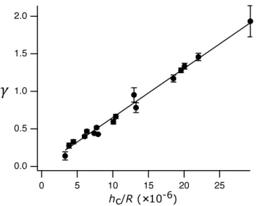
That is why, the 𝛾 factor was then calculated to fit the measured the initial lubricant film thickness at the first stages of the oscillating motion over 88 deceleration/acceleration experiments. It was then plot-ted against the dimensionless Hamrock–Dowson film thickness ℎC∕𝑅

calculated with the velocity amplitude 𝑢₀ (Fig. 7). As a result, the 𝛾 factor is linear with the Hamrock–Dowson film thickness with a

coefficient of determination of 98.9%, meaning that it is proportional to 𝐿3∕4_∕𝑀7∕9 = √_𝛾 𝑟 1+𝑟𝛾 with ⎧ ⎪ ⎨ ⎪ ⎩ if 𝑆 ≤ 0, 𝑟 = 𝐻2𝑛−1(𝑋m) ̄ 𝜌(𝑃 )⋅𝐻2𝑛(0) else 𝑟 = 𝐻2𝑛−1(𝑋1) ̄ 𝜌(𝑃 )⋅𝐻2𝑛(0) and { 𝛾= (6.50.1) × 104 ⋅ ℎC∕𝑅 ℎ_{C∕𝑅 = 1.92 ⋅ 𝑈}0.67 ⋅ 𝐺0.53⋅ 𝑊−0.067 (7)

Eventually, the central film thickness of various lubricated contacts in time-varying conditions can be accurately calculated (Fig. 8). As shown by the waterfall representations (Fig. 8a and b), the calculation using the starvation factor gives similar variations and values of lubri-cant thickness profiles as during the experiments. On the one hand, the

Fig. 7. 𝛾 factor as a function of the dimensionless Hamrock–Dowson film thickness

ℎC∕𝑅.

deviation of calculation from experiment increased for positions further away from the contact center. This was presumably due to the strong assumptions, i.e. Ertel hypotheses and Crooks? approximation, used for the analytical resolution. This could also originate from the triangular velocity profile. On the other hand, the calculated central film thickness shows an accurate reproduction of the measurement (Fig. 8c). In partic-ular, the film thickness inflexions previously observed around the zero velocity and between each acceleration and deceleration was clearly retrieved here by the calculation.

5. Conclusions

The film establishment mechanisms in EHL regime in forced os-cillations were investigated thanks to the full-analytical resolution of the Reynolds equation. This solution was backed-up with experimen-tal measurements using the CHRONOS tribometer which permits di-rect contact visualization under controlled forced oscillations. Con-sequently, the main contributions to the film establishment i.e. the squeeze and the transport effect, were well retrieved by the calculation, which confirms several observations:

• The lubricant film thickness hysteresis in the contact as its evolu-tion was asymmetric during an acceleraevolu-tion and a deceleraevolu-tion. Therefore, the maximum film thickness was not synchronized with the maximum velocity and the minimum film thickness did not occur at the zero velocity.

• A slight drop of film thickness was observed around the zero velocity due to the transient squeeze ad residence time effect which depend on the dimensionless time parameter 𝜎.

• Between each deceleration and acceleration, a lubricant film thickness inflection was observed due to the inlet flow reduction at the change in direction. This effect was well considered in the calculation using an adaptation of Chevalier’s film thickness reduction parameter with an adjustment of the 𝛾 factor as a function of the film thickness.

Declaration of competing interest

The authors declare that they have no known competing finan-cial interests or personal relationships that could have appeared to influence the work reported in this paper.

Fig. 8. Lubricant film thickness for a viscosity of 0.8 Pa s and sliding frequency of 10 Hz under a load of 10 N: (a) waterfall of calculated profiles; (b) waterfall of measured profiles;

CRediT authorship contribution statement

M. Yahiaoui: Investigation, Data curation, Validation, Formal anal-ysis, Software, Writing - original draft, Writing - review & editing, Vi-sualization. D. Mazuyer: Conceptualization, Methodology, Validation, Formal analysis, Writing - review & editing, Supervision. J. Cayer-Barrioz: Conceptualization, Methodology, Resources, Writing - review & editing, Supervision, Project administration, Funding acquisition. Acknowledgments

This work was performed at the Laboratoire de Tribologie et Dy-namique des Systèmes, Ecole Centrale de Lyon, CNRS UMR5513. It was funded by the French Agence Nationale de la Recherche under the Confluence Project No. ANR-13-JS09-0016-01.

References

[1] Brizmer V, Kligerman Y, Etsion I. A laser surface textured parallel thrust bearing. Tribol Trans 2003;46:397–403.

[2] Mourier L, Mazuyer D, Lubrecht AA, Donnet C. Transient increase of film thickness in micro-textured EHL contacts. Tribol Int 2006;39:1745–56.

[3] Mourier L, Mazuyer D, Ninove FP, Lubrecht AA. Lubrication mechanisms with laser-surface-textured surfaces in elastohydrodynamic regime. Proc Inst Mech Eng J 2010;224:697–711.

[4] Mazuyer D, Varenne E, Lubrecht AA, Georges J-M, Constans B. Shearing of adsorbed polymer layers in an elastohydrodynamic contact in pure sliding. In: Dowson D, et al., editors. Lubrication at the frontier 1999. Elsevier Science B.V.; 1999, p. 493–504.

[5] Meunier C. Vieillissement des lubrifiants et compréhension des mécanismes de dégradation: Application à la zone segment-piston-chemise (Ph.D. Thesis), Ecole centrale de Lyon, ECL; 2008, p. 2008–29.

[6] Ernesto A, Mazuyer D, Cayer-Barrioz J. The combined role of soot aggrega-tion and surface effect on the fricaggrega-tion of a lubricated contact. Tribol Lett 2014;55:329–41.

[7] Ernesto A, Mazuyer D, Cayer-Barrioz J. From full-film lubrication to boundary regime in transient kinematics. Tribol Lett 2015;59(1):1–10.

[8] Hooke CJ. The minimum film thickness in lubricated line contacts during a reversal of entrainment – General solution and development of a design chart. Proc Inst Mech Eng 1994;208:53–64.

[9] Sugimura J, Spikes HA. Technique for measuring EHD film thickness in non steady-state contact conditions. In: Dowson D, et al., editors. Elastohydrodynamics 1996. Elsevier Science B.V.; 1997, p. 91–100.

[10] Sugimura J, Jones Jr WR, Spikes HA. EHD film thickness in non-steady state contacts. Trans ASME 1998;120:442–52.

[11] Sugimura J, Okumura T, Yamamoto Y, Spikes HA. Simple equation for EHL film thickness under acceleration. Tribol Int 1999;32:117–23.

[12] Glovnea R, Spikes HA. Behavior of EHD films during reversal of entrainment in cyclically accelerated/decelerated motion. Tribol Trans 2002;45:177–84.

[13] Wang J, Hashimoto T, Nishikawa H, Kaneta M. Pure rolling elastohyddrodynamic lubrication of short stroke reciprocating motion. Tribol Int 2005;38:1013–21.

[14] Bassani R, Ciulli E, Carli M, Stadler K. Experimental investigation of transient and thermal effects on lubricated non-conformal contacts:. Tribotest 2007;13:183–94.

[15] Ciulli E. Non-steady state non-conformal contacts: friction and film thickness studies. Meccanica 2009;44:409–25.

[16] Hamrock BJ, Dowson D. Isothermal elastohydrodynamic lubrication of point contacts: Part III - fully flooded results. J Lubr Technol 1977.

[17] Nijenbanning G, Venner CH, Moes H. Film thickness in elastohydrodynamically lubricated elliptic contacts. Wear 1994;176:217–29.

[18] Ohno N, Yamada S. Effect of high-pressure rheology of lubricants upon entrapped oil film behaviour at halting elasto- hydrodynamic lubrication. Proc Inst Mech Eng J 2007;221:279–85.

[19] Mazuyer D, Ernesto A, Cayer-Barrioz J. Theoretical modeling of film-forming mechanisms under transient conditions: Application to deceleration and experimental validation. Tribol Lett 2017;65:22–36.

[20] Petrousevitch AI, Kodnir DS, Salukvadze RG, Bakashvili DL, Schwarzman VSH. The investigation of oil film thickness in lubricated ball-race rolling contact. Wear 1972;19:369–89.

[21] Yahiaoui M, Rigaud E, Mazuyer D, Cayer-Barrioz J. Forced oscillations dynamic tribometer with real-time insights of lubricated interfaces. Rev Sci Instrum 2017;88. 035101.

[22] Wedeven LD, Evans D, Cameron A. Optical analysis of ball bearing starvation. In: ASME conference. 1970.

[23] Chiu YP. An analysis and prediction of lubricant film starvation in rolling contact systems. ASLE Trans 1974;17:22–35.

[24] Pemberton J, Cameron A. A mechanism of fluid replenishment in elastohydro-dynamic contacts. Wear 1976;37:185–90.

[25] Kingsbury E. Parched elastohydrodynamic lubrication. J Tribol 1985;107:229–32.

[26] Chevalier F. Modélisation des conditions d’alimentation dans les contacts elastohydrodynamiques ponctuels (Ph.D. Thesis), INSA Lyon; 1996.

[27] Chevalier F, Lubrecht AA, Cann PME, Dalmaz G. The evolution of lubricant film defects in the starved regime. In: Tribology for energy conservation, Proceedings of the 24th Leeds-Lyon symposium in tribology, Vol. 34. 1998, p. 233–42.

[28] Damiens B. Modélisation de la lubrification sous-alimentée dans les contacts elastohydrodynamiques elliptiques (Ph.D. Thesis), INSA Lyon; 2003.

[29] Touche T, Woloszynski T, Podsiadlo P, Stachowiak GW, Cayer-Barrioz J, Mazuyer D. Numerical simulations of groove topography effects on film thickness and friction in EHL regime. Tribol Lett 2017;65:113.

[30] Chevalier F, Lubrecht AA, Cann PME, Dalmaz G. Film thickness in starved EHL point contacts. J Tribol 1998;120:126–33.

[31] Damiens B, Venner CH, Cann PME, Lubrecht AA. Starved lubrication of elliptical EHD contacts. J Tribol 1998;120:126–33.