Impact of interactive vegetation phenology on the simulated pan-arctic land surface state

UNIVERSITÉ DU QUÉBEC À MONTRÉAL

IMPACT OF INTERACTIVE VEGETATION PHENOLOGY ON THE SIMULATED PAN-ARCTIC LAND SURFACE STATE

DISSERTATION PRESENTED

AS PARTIAL REQUIREMENT

FOR MSC DEGREE IN A TMOSPHERIC SCIENCES

BY

BERNARDOSTEPHANTEUFEL

Avertissement

La diffusion de ce mémoire se fait dans le respect des droits de son auteur, qui a signé le formulaire Autorisation de reproduire et de diffuser un travail de recherche de cycles supérieurs (SDU-522 - Rév.0?-2011). Cette autorisation stipule que «conformément à l'article 11 du Règlement no 8 des études de cycles supérieurs, [l'auteur] concède à l'Université du Québec à Montréal une licence non exclusive d'utilisation et de publication de la totalité ou d'une partie importante de [son] travail de recherche pour des fins pédagogiques et no'n commerciales. Plus précisément, [l'auteur] autorise l'Université du Québec à Montréal à reproduire, diffuser, prêter, distribuer ou vendre des copies de [son] travail de recherche à des fins non commerciales sur quelque support que ce soit, y compris l'Internet. Cette licence et cette autorisation n'entraînent pas une renonciation de [la] part [de l'auteur] à [ses] droits moraux ni à [ses] droits de propriété intellectuelle. Sauf entente contraire, [l'auteur] conserve la liberté de diffuser et de commercialiser ou non ce travail dont [il] possède un exemplaire.>>

UNIVERSITÉ DU QUÉBEC À MONTRÉAL

EFFETS DE L'INCLUSION DE LA PHÉNOLOGIE INTERACTIVE DE LA VÉGÉTATION SUR L'ÉTAT DE SURF ACE SIMULÉ DU DOMAINE

PAN ARCTIQUE

MÉMOIRE PRÉSENTÉ

COMME EXIGENCE PARTIELLE

DE LA MAÎTRISE EN SCIENCES DE L'ATMOSPHÈRE

PAR

BERNARDO STEPHAN TEUFEL

TABLE OF CONTENTS LIST OF FIGURES ... v RÉSUMÉ ... vii ABSTRACT ... .' ... ix CHAPTERI INTRODUCTION ... ! 1.1 Context ... 1

1.2 Objective and methods ... 7

CHAPTER II IMPACT OF INTERACTIVE VEGETATION PHENOLOGY ON THE SIMULA TED PAN-ARCTIC LAND SURF ACE STA TE ... 11

2.1 Introduction ... 13 2.2 Methods ... 16 2.2.1 Mode! description ... 16 2.2.2 Experiments ... 18 2.2.3 Soil properties ... 21 2.2.4 Spatial distribution of PFTs ... 22 2.2.5 Validation data ... 23 2.3 Results ... : ...... 25 2.3 .1 Validation ... 25

2.3 .2 Impact of deep soi! çolumn ... 27

2.3.3 Impact of interactive phenology (recent past) ... 29

2.3 .4 Impact of interactive phenol ogy on projected changes ... 31

2.4 Summary and conclusions ... 33

FIGURES ... 37 CHAPTERIII

CONCLUSION ... 49 APPENDIXA

SUPPLEMENTARY FIGURES ... 53 REFERENCES ... 61

LIST OF FIGURES

Figure Page

2.1 Number of prescribed organic soillayers : dark blue is used for grid cells with 0 layers, cyan for 1 layer (1 0 cm), yellow for 2 layers (30 cm) and red for deep organic soils ... 37 2.2 Prescribed fractional coverages of plant functional types: (a) needleleaf

evergreen trees, (b) needleleaf deciduous trees, ( c) broadleaf deciduous trees, (d) crops, (e) grasses, (f) bare soil... ... 38 2.3 Mean PAl [m2 m·2] for the 1982-1998 period from (a)

CLASS26_CTEM/ERA, (b) ISLSCP Il ... 39 2.4 Mean NPP (kgC m-2 yr-1] for the 2000-2010 period from (a)

CLASS26_CTEM/ERA, (b) MODIS ... 39 2.5 Soi! carbon density [kg m-2] from (a) CLASS26_CTEM/ERA for the

1981-1990 period, (b) IGBP, (c) NCSCD ... .40 2.6 (a) Mean 1981-1990 active layer thickness [ m] of near-surface permafrost,

simulated by CLASS26 _ CTEM/ERA. (b) Observed permafrost extent: magenta, continuous (>90%); blue, discontinuous (50-90%); green, sporadic (10-50%); yellow, isolated (<10%) ... 40 2.7 Comparison between modelled and observed ALT [rn] for the 1990-2012

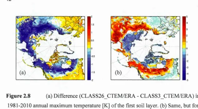
period. Here blue circles are used for CLASS26_CTEM/ERA and green triangles for CLASS26/ERA ... 41 2.8 (a) Difference (CLASS26_CTEM/ERA -CLASS3_CTEM/ERA) in

1981-2010 annual maximum temperature [K] of the first soil layer. (b) Same, but for annual minimum temperature ... 42 2.9 (a) Difference (CLASS26_CTEM/ERA- CLASS3_CTEM/ERA) in

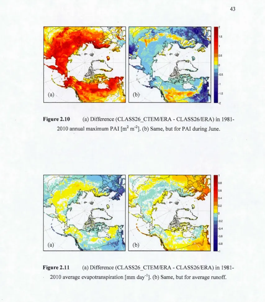
1981-2010 annual maximum PAl [m2 m-2]. (b) Same, but for average root zone moisture availability (adimensional : equal to zero at the wilting point and below, equal to one at field capacity and above). ... .42 2.10 (a) Difference (CLASS26_CTEM/ERA- CLASS26/ERA) in 1981-2010

2.11 (a) Difference (CLASS26_CTEM/ERA-CLASS26/ERA) in 1981-2010 average evapotranspiration [mm day-1]. (b) Same, but for average runoff ... 43 2.12 (a) Difference (CLASS26_CTEM/ERA- CLASS26/ERA) in 1981-2010

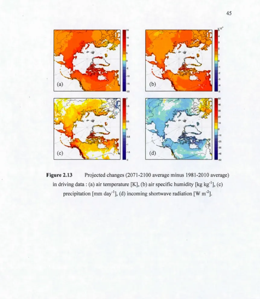
summer temperature [K] of the first soillayer. (b) Same, but for ALT [rn]. 44 2.13 Projected changes (2071-2100 average minus 1981-2010 average) in driving

data: (a) air temperature [K], (b) air specifie humidity [kg kg-1], (c)

precipitation [mm day-1], (d) incoming shortwave radiation [W m-2]. •••••••••• 45 2.14 Projected changes (2071-2100 minus 1981-2010) in : (a,b) spring PAl [m2

m-2], (c,d) spring ET [mm day-1], (e,f) ALT [rn], from

CLASS26_CTEM/CRCM in the first column (a,c,e), and from

CLASS26/CRCM in the second column (b,d,f). Grey areas in (e,f) represent regions where permafrost in the top 5 meters of soi! degraded completely by 2071-2100 ... 46 2.15 Differences (CLASS26_CTEM/CRCM- CLASS26/CRCM) in ALT [rn] for

the (a) 1981-2010 period, (b) 2011-2040, ( c) 2041-2070, ( d) 2071-2100 .... 4 7 A.1 (a) Difference (CLASS26_CTEM/ERA- CLASS3_CTEM/ERA) in

1981-2010 winter (DJF) temperature [K] of the first soi! layer. (b) Same, but for spring (MAM). (c) Same, but for summer (JJA). (d) Same, but for fall

(SON) ... 54 A.2 (a) Difference (CLASS26_CTEM/ERA-CLASS26/ERA) in 1981-2010

winter (DJF) PAl [m2 m-2]. (b) Same, but for spring (MAM). (c) Same, but for summer (JJA). (d) Same, but for fall (SON) ... 55 A.3 (a) Difference (CLASS26_CTEM/ERA- CLASS26/ERA) in 1981-2010

winter (DJF) evapotranspiration [mm day-1]. (b) Same, but for spring

(MAM). (c) Same, but for summer (JJA). (d) Same, but for fall (SON) ... 56 A.4 (a) Difference (CLASS26_CTEM/ERA- CLASS26/ERA) in 1981-2010

winter (DJF) temperature [K] of the first soi! layer. (b) Same, but for spring (MAM). (c) Same, but for summer (JJA). (d) Same, but for fall (SON) ... 57 A.5 (a) Projected changes (2071-2100 minus 1981-2010) in winter (DJF) driving

air temperature [K]. (b) Same, but for spring (MAM). (c) Same, but for summer (JJA). (d) Same, but for fall (SON) ... 58 A.6 (a) Projected changes (2071-2100 minus 1981-2010) in winter (DJF) driving precipitation [mm day-1]. (b) Same, but for spring (MAM). (c) Same, but for summer (JJA). (d) Same, but for fall (SON) ... 59

RÉSUMÉ

Dans la région panarctique, la surface terrestre subit des changements rapides causés par le réchauffement climatique. Le pergélisol près de la surface devrait se dégrader de manière importante au cours du 21 e siècle, provoquant des rétroactions sur le climat mondial et les cycles de l'eau à l'échelle régionale. La réponse de la végétation au réchauffement climatique et à l'augmentation des concentrations atmosphériques de C02 va influencer l'ampleur de ces rétroactions. Dans cette étude, l'impact de la phénologie interactive sur l'état de la surface terrestre est évalué en _comparant d_eux simulations du schéma canadien de surface (CLASS) - une avec phénologie interactive, modélisée en utilisant le modèle canadien des écosystèmes terrestres (CTEM), et 1 'autre avec phénologie prescrite. Ces simulations sont réalisées pour la période de 1979 à 2012, en utilisant le forçage atmosphérique de la réanalyse ERA-Interim. Les valeurs simulées de l'indice de surface foliaire, la productivité primaire, l'étendue du pergélisol et 1 'épaisseur de la couche active sont comparées aux observations disponibles. Les résultats suggèrent que les deux simulations capturent la distribution générale de la végétation et du pergélisol, bien que certaines erreurs demeurent. Des différences significatives dans 1 'évapotranspiration sont observées entre les deux simulations, conduisant à des différences dans le ruissellement, la température du sol et 1 'épaisseur de la couche active. Pour évaluer l'impact de la phénologie interactive sur les changements prévus dans l'état de la surface terrestre, deux autres simulations sont comparées, l'une avec CLASS et l'autre avec CLASS couplé à CTEM, en utilisant le forçage atmosphérique d'une simulation transitoire du modèle régional canadien du climat (MRCC5) pour le scénario RCP8.5. Ces deux simulations montrent une dégradation importante du pergélisol près de la surface, mais la simulation avec phénologie interactive montre une perte légèrement plus rapide du pergélisol, pointant vers une rétroaction positive de la végétation sur la température du sol.

Mots-clés: modèle dynamique de la végétation, pergélisol, épaisseur de la couche active, carbone du sol, changement climatique

ABSTRACT

The pan-Arctic land surface is undergoing rapid changes caused by a warming climate. Near-surface permafrost is projected to degrade significantly during the 21st

century, resulting in feedbacks to global climate and regional water cycles.

Vegetation response to the warming climate and increasing atmospheric C02

concentrations will influence the magnitude of these feedbacks. In this study, the

impact of interactive phenology on the land surface state is assessed by comparing two simulations of the Canadian Land Surface Scheme (CLASS) - one with

interactive phenology, modelled using the Canadian Terrestrial Ecosystem Model

(CTEM), and the other with prescribed phenology. These simulations are performed for the 1979-2012 period, using atmospheric forcing from the ECMWF ERA-Interim

reanalysis. Simulated plant area index, primary productivity, permafrost and active

layer thickness are compared to available observational estimates. Results suggest that both simulations capture the general distribution of vegetation and permafrost,

although sorne biases remain. Significant differences in evapotranspiration are

observed between both simulations, leading to differences in runoff, soil temperature

and active layer thickness. To assess the impact of interactive phenol ogy on projected

changes to the land surface state, two further simulations are compared, one with

CLASS and the other with CLASS coupled to CTEM, both driven by atmospheric

forcing data from a transient climate change simulation of the 5th generation Canadian Regional Climate Model (CRCM5) for the Representative Concentration Pathway 8.5. Both of these simulations show extensive near-surface permafrost

degradation, but the simulation with interactive phenology shows slightly faster

permafrost loss, painting towards a positive feedback of vegetation on soil

temperatures.

Keywords : dynamic vegetation model, permafrost, active layer thickness, soil carbon, climate change

CHAPTERI

INTRODUCTION

1.1 Context

Human activities are affecting the Earth's energy budget by changing the atmospheric concentrations of greenhouse gases and aerosols and by changing land surface properties. Carbon dioxide concentrations have increased by 40% since pre-industrial times, primarily from fossil fuel emissions, and have reached levels not seen in the last 800,000 years. The combined effect of these changes has been an uptake of energy by the climate system, resulting in wanning of the atmosphere and the ocean, diminishing snow and ice, and rising sea levels (IPCC, 2013).

Climate models, based on the fundamental laws of nature (e.g., energy, mass and momentum conservation), are the primary tools available to investigate the response of the climate system to various forcings and to make projections of future climate. Models are able to reproduce the observed continental-scale surface temperature patterns and trends over many decades, and conclude that continued emissions of greenhouse gases will cause further warming and changes in ail components of the climate system (IPCC, 2013).

Regional downscaling methods provide climate infonnation at the smaller scales needed for many climate impact studies, as the horizontal resolution of global models is often too low to resolve features that are important at regional scales (IPCC, 2013). Regional climate models (RCMs) are applied over a limited-area

domain with boundary conditions either from global reanalyses or global climate mode! output (Laprise, 2008). Downscaling by RCMs adds value mainly in regions with highly variable topography and for various small-scale phenomena (Di Luca et al., 2012; Feser et al., 2011).

One region undergoing rapid changes is the Arctic land surface, which has warmed at a rate of 0.5°C per decade over the past three decades. This rate is significantly higher than the global average wanning rate, due to a characteristic of the climate system known as Arctic amplification (IPCC, 20 13). Temperatures over the Arctic during the past few decades have been significantly higher than those seen over the past 2000 years (Kaufman et al., 2009).

Arctic amplification has a number of causes, with albedo feedback playing an important role both over the land surface and over the ocean (Serreze and Barry, 2011 ). Albedo feedback is a positive feedback cycle in which the albedo decreases as highly reflective ice and snow melt, exposing the darker and more absorbing surfaces below and the additional absorbed heat causes further melting. Other positive feedbacks contributing on longer tirne scales are associated with vegetation changes and thawing permafrost (IPCC, 2013).

Arctic amplification is evident in both the instrumental records and climate model projections through the 21 st century (Serreze and Barry, 2011 ). However, the magnitude of the projected warming strongly depends on assumptions about future greenhouse gas emissions. One possibility is that emissions will continue to increase during the 21 st century, which is represented by the Representative Concentration Pathway 8.5 (RCP8.5). Under this scenario, Arctic warming is expected to exceed the global average (2.6 to 4.8°C) by 2.2 to 2.4 times by the end of the 21st century, irnplying that Arctic temperatures would continue to rise at an average rate of at least 0.5°C per decade (IPCC, 2013).

3

This ongoing Arctic warming directly affects the cryosphere, as evidenced by decreases of more than 10% per decade in Arctic perennial sea-ice extent since 1979 (IPCC, 2013). Over land, Arctic warming affects the Greenland ice sheet, glaciers and permafrost, which is defmed as ground (soi! or rock) that remains at or be1ow 0°C for two or more consecutive years. Permafrost was estimated to underlay about 24% of the northern hemisphere land surface during the second half of the 20th century (Zhang et al., 2008).

Given the strong projected warmmg across the northern high latitudes, substantial near-surface permafrost degradation is expected during the 21 st century (Slater and Lawrence, 2013). Permafrost degradation at greater depths occurs much more slowly, but is Jess relevant to the surface energy and water balance (Delisle, 2007). Following the RCP8.5 scenario, a reductioN of around 80% by the end of the 21st century in near-surface permafrost area (areas with permafrost in the top 3.5 rn of soi!) is projected by the CMIP5 models (Koven et al., 2013; Slater and Lawrence, 2013).

As mentioned previously, the main driver of global warming is the increase in the concentration of greenhouse gases in the atmosphere. However, the concentration of greenhouse gases is also strongly dependant on the global carbon cycle, where soi! respiration plays an important role. Soi! respiration is the process in which carbon dioxide (C02) is produced in soils by roots and soi! organisms and subsequently released to the atmosphere. Increased soi! respiration with global warming is likely to provide a positive feedback to the greenhouse effect (Raich and Schlesinger, 1992).

J

Close to 1700 Pg of soi! carbon are stored in the northern circumpolar permafrost zone, more than twice as much carbon than in the atmosphere (Tarnocai et al., 2009). This soi! carbon accumulated over thousands of years under cold conditions (Schuur et al., 2013). As permafrost thaws, this soi! carbon may become

active, leading to emission of greenhouse gases such as methane or carbon dioxide, depending on the amount ofwater in the soil (Lawrence and Slater, 2005).

There are no direct measurements of soi! carbon Ioss from the permafrost zone at large scales. This is in part due to a scarcity of soil carbon measurements in this region, in combination with an overall difficulty of detecting changes in soil carbon pools due to large soil heterogeneity (Schuur et al., 2013).

According to the latest mode] projections, around 15% of the simulated permafrost carbon pool is expected to be lost as greenhouse gas emissions by 2100 following the RCP8.5 scenario. Independent estimates from laboratory experiments and assessment by experts agree on 5% to 15% of the permafrost carbon pool being vulnerable under this scenario (Schuur et al., 2015). Future projections of permafrost and soil carbon remain Iimited given the Iack of representation of processes within current models. Even if processes are included, validating them is often problematic due to the scarcity of actual measurements from these remote landscapes. Nevertheless, the release of carbon from permafrost zone soils is Iikely to influence the pace of climate change in the 21 st century and beyond. However, fossil fuel burning is likely to continue to be the main source of carbon emissions and climate forcing (Schuur et al., 2013).

Fire could be an important additional mechanism for releasing permafrost carbon to the atmosphere. Fire frequency and severity are increasing in sorne parts of the boreal permafrost zone. Thawing and tires could act together to expose and transfer permafrost carbon to the atmosphere very rapidly, especially in ecosystems with organic surface soils (Turetsky et al., 201 0).

In addition to affecting the global carbon budget, permafrost thaw alters soil structural and hydrologie properties, with impacts on the spatial extent of lakes and wetlands (Smith et al., 2005) and possibly on the freshwater fluxes to the Arctic

5

ocean (Lawrence and Slater, 2005). Increasing winter base flow and mean annual

stream flow resulting from possible permafrost thawing were reported in northwest Canada (St. Jacques and Sauchyn, 2009). Rjsing minimum daily flows also have been

observed in northern Eurasian ri vers (Smith et al., 2007). Changes in the amount of

freshwater reaching the Arctic Ocean affect sea-ice formation and may alter the

oceanic thermohaline circulation (Amel!, 2005).

An imp·ortant factor to consider when studying warming and its impacts on

permafrost is the role of vegetation changes in future climate. lt is known that the

distribution of natural vegetation is govemed primarily by clirnate, through

precipitation, temperature and radiation (Nemani et al., 2003; Stephenson, 1990).

Vegetation variability is driven by climate, through heat/cold stress, drought stress

and light. Observations show that temperature is important for forcing vegetation

variability in the northern mid/high latitudes while precipitation is important in the

tropics and subtropics (Liu et al., 2006).

Specially relevant to permafrost degradation is the fact that vegetation also

influences climate, through the biophysical and biogeochemical pathways, where the

biogeochemical impacts are via modifying the atmospheric C02 concentrations, while

the biophysical pathway influences climate through impacts on surface albedo and on

the land-atrnosphere fluxes of energy, water and momentum. Vegetation growth and

expansion tends to lower the surface albedo, resl!lting in more energy absorption.

When snow is present, this change in albedo is even larger (Liu et al., 2006).

The height of vegetation strongly influences surface roughness. Increases in

surface roughness are associated with an increase in the efficiency with which

sensible heat is transferred from the surface to the atmosphere. Changes in surface

roughness can also influence precipitation and large-scale circulation patterns

Observations show that the vegetation feedback on climate is less significant than the climate forcing on vegetation. A strong positive feedback of vegetation on temperature, explaining 10% to 25% of the interannual temperature variance, is observed in the northem mid/high latitudes. The vegetation feedback adds moisture to the atmosphere locally, but the increased moisture might not precipitate locally, resulting in insignificant feedbacks on precipitation, except for sorne isolated semiarid pockets in the tropics/subtropics (Liu et al., 2006).

The biophysical feedbacks are controlled by mechanisms ofregiona1 character and the relative importance of individual feedback mechanisms might differ among regions (Quillet et al., 201 0; Wramneby et al., 201 0).

Recent warming trends have been associated with earlier onset of vegetation activity in spring, delayed autumn senescence and an overall extension in the length of the active growing season. In high latitude ecosystems, two factors regulate the spring onset: the timing of snowmelt and the temperatures that follow snowmelt. The timing depends on the depth of the winter snowpack and on springtime temperatures. If the snow melts too early, plants might be exposed to cold air temperatures that inhibit development or cause frost damage (Richardson et al., 2013).

Increased atmospheric C02 promotes stomatal closure and reduced transpiration (Field et al., 1995). On the other hand, higher temperatures increase the atmospheric demand for water, increasing evapotranspiration (Wramneby et al., 201 0). There is potential for substantial feedbacks between vegetation changes and regional water cycles, but the impact of such feedbacks remains uncertain due to limitations in modelling vegetation processes and uncertainties in plant response, ecosystem shifts and land management changes (IPCC, 2013).

A greater availability of C02 might increase photosynthesis. Nutrient availability and soi! moisture conditions play an important role in this response

7

(Quillet et al., 201 0). The physiological effects of COz on productivity and water-use

efficiency decrease with increasing COz concentration, approaching an asymptote at

high COz concentrations (Cramer et al., 2001 ).

Global warming will alter the density of vegetation cover, modifying the

physical characteristics of the land surface (Betts et al., 1997). An assessment of changes in plant productivity, inferred from satellite observations between 1982 and

2012 shows that about a third of the pan-Arctic has substantially greened, less than

4% browned, and more than 57% did not change significantly (Xu et al., 20 13).

Severa! studies have calculated the magnjtude of the combined effects of

vegetation change in the Arctic, including the negative feedbacks of COz

sequestration and increased evapotranspiration and the positive feedback of decreased

albedo. lt is likely that vegetation changes will result in an overall positive feedback

to Arctic warming (Pearson et al., 2013; Swann et al., 2010; Wramneby et al., 2010;

Zhang et al., 2014), thus favouring near-surface permafrost degradation and its

associated impacts on regional hydrology.

1.2 Objective and methods

In order to gain insight into the processes occurring at the land surface in high

latitude regions, offline simulations using the Canadian Land Surface Scheme (CLASS) coupled to the Canadian Terrestrial Ecosystem Model (CTEM) are performed over a pan-Arctic domain. These simulations are first performed for the recent past (1979 - 2012), using reanalysis data to drive the models. In a second phase, output from an existing simulation of the 5th generation Canadian Regional Climate Model (CRCM5) is used to drive the models in a climate change (1961

As this is the ftrst time that CLASS and CTEM are used together over a pan-Arctic domain at 0.5 degrees resolution, an assessment of their performance in simulating vegetation, soi! carbon and permafrost is necessary. This assessment is performed by comparing model output to observational estimates of severa! key variables. In order to facilitate this assessment only the basic modules of CTEM are used, which requires the spatial distribution of plant functional types to be prescribed and time-invariant. As the term dynamic vegetation is commonly reserved for models where vegetation can expand horizontally (in addition to vertical growth), the term interactive vegetation phenology is used in this study to represent vegetation that can only grow vertically, following Garnaud et al. (20 14b).

CLASS and CTEM were originally designed to use a soi! column consisting of only 3 vertical layers, extending to a depth of 4.1 m. It was shown by Paquin and S ushama (20 14) that su ch soi 1 depths were insufficient to realistically represent permafrost, a key component of the land surface in the pan-Arctic. As the same study showed that a soi! depth of 60 rn provided a much better representation of permafrost, it became necessary to use such a deep soil configuration for the present study.

In light of this, a first sensitivity study consists in analyzing the effects of a deep soil configmation on the land surface and on vegetation, which is performed by comparing a simulation of CLASS coupled to CTEM with the original 3 layer configmation to a simulation with a 26 layer configuration, both driven by reanalysis data. This comparison starts by loo king at the differences in the thermal regime of the soi!, which drives the differences in ali other components of the land smface.

The main sensitivity study of this work consists in analyzing the differences between simulations using CLASS coupled to CTEM and simulations using only CLASS. As ali these simulations are performed using the deep soil configmation and starting from the same initial conditions, the differences between them originate from the way vegetation is represented within each model.

9

When CLASS is not coupled to CTEM only the seasonality of vegetation is represented in CLASS, with plant area index (P AI) varying between an annual maximum and minimum P AI, which are prescribed along with all other vegetation related parameters, such as roughness length, rooting depth and canopy mass. When . CLASS is coup led to CTEM, vegetation can ad apt to climate and P AI as well as ail other vegetation parameters are dynamic functions of climate, soil conditions and

co2 concentrations.

The sensitivity of the simulated land surface to interactive phenology (i.e. CTEM) is first assessed for the simulations driven by reanalysis data, linking the differences between the simulations to differences in P AI and evapotranspiration,

which are the main variables affected by intr~ducing CTE~. In a second phase, this sensitivity is also assessed for the simulations driven by CRCM5 output. In this case,

the response of the land surface and vegetation to projected climate change is analyzed, and the effect of including interactive phenology on permafrost and other components is assessed.

The objectives of this work can be summarized as follows :

• Assess the quality of the simulations produced by CLASS coupled to CTEM over the pan-Arctic domain, by comparing the simulated vegetation, soil carbon and permafrost to observational estimates.

• Analyze the impact of using a deep soil configuration on the simulated pan-Arctic land surface state and vegetation.

• Analyze the impact of using interactive phenology on the simulated pan-Arctic land surface state, for the recent past and for a climate change scenano.

This work is organized as follows : chapter one presents the context of the research, along with a summary of the methods used and the objectives of this study.

Chapter two presents the main results of this study, in the form of an article to be submitted to a scientific journal, including an introduction in section 2.1, methods in section 2.2, results in section 2.3 and conclusions in section 2.4. Chapter three presents a brief summary of the results and conclusions.

CHAPTERII

IMPACT OF INTERACTIVE VEGETATION PHENOLOGY ON THE

SIMULATED PAN-ARCTIC LAND SURFACE STATE

Bernardo Teufel1,., Laxmi Sushama1, Vivek K. Arora2, Diana Verseghy1'3

1

Centre ESCER (Étude et Simulation du Climat à l'Échelle Régionale), University of Quebec at Montreal, 201-President-Kennedy, Montreal, Canada

2

Canadian Centre for Climate Modelling and Analysis, Climate Research Division,

Environment Canada, University of Victoria, Victoria, Canada 3

Climate Processes Section, Climate Research Division, Environment Canada, Toronto, Canada

*Corresponding author

Tel: +1 514-987-3000 ext. 2414 Fax : + 1 514-987-6853

E-mail : teufel@sca.uqam.ca

Abstract

The pan-Arctic land surface is undergoing rapid changes caused by a warming climate. Near-surface permafrost is projected to degrade significantly during the 21 st century, resulting in feedbacks to global climate and regional water cycles. Vegetation response to the warming climate and increasing atmospheric C02 concentrations will influence the magnitude of these feedbacks. In this study, the impact of interactive phenology on the land surface state is assessed by comparing two simulations of the Canadian Land Surface Scheme (CLASS) - one with interactive phenology, modelled using the Canadian Terrestrial Ecosystem Mode! (CTEM), and the other with prescribed phenology. These simulations are performed for the 1979-2012 period, using atmospheric forcing from the ECMWF ERA-Interim reanalysis. Simulated plant area index, primary productivity, permafrost and active layer thickness are compared to available observational estimates. Results suggest that both simulations capture the general distribution of vegetation and permafrost, although sorne biases remain. Significant differences in evapotranspiration are observed between both simulations, leading to differences in runoff, soil temperature and active layer thickness. To assess the impact of interactive phenology on proj~cted changes to the land surface state, two further simulations are compared, one with CLASS and the other with CLASS coupled to CTEM, both driven by atmospheric forcing data from a transient climate change simulation of the 5th generation Canadian Regional Climate Mode! (CRCM5) for the Representative Concentration Pathway 8.5. Both of these simulations show extensive near-surface permafrost degradation, but the simulation with interactive phenology shows slightly faster permafrost Joss, painting towards a positive feedback of vegetation on soil temperatures.

Keywords : dynamic vegetation mode!, permafrost, active layer thickness, soil carbon, climate change

13

2.1 Introduction

Over the past three decades the Arctic land surface has warmed at a rate of 0.5°C per decade, which is significantly higher than the global average warming rate (IPCC, 2013). This Arctic amplification has a number of causes, with albedo feedback playing an important role (Serreze and Barry, 2011). Other positive feedbacks contributing on longer time scales are associated with vegetation changes and thawing permafrost (IPCC, 2013). According to the fifth assessment report of the IPCC (2013), Arctic temperatures are projected to continue to rise at an average rate of at least 0.5°C per decade under the Representative Concentration Pathway 8..5 (RCP8.5) scenario.

This ongoing Arctic warming affects permafrost, which is defined as ground that remains at or below 0°C for two or more consecutive years. Permafrost is estimated to underlay about 24% of the northem hemisphere land surface (Zhang et

al., 2008). Given the strong projected warming across the northern high latitudes, substantial near-surface permafrost degradation is expected during the 21 st century. For instance, following the RCP8.5 scenario, a reduction of around 80% in the near -surface permafrost area (i.e. permafrost in the top 3.5 rn below surface) is projected by Koven et al. (2013) and Slater and Lawrence (2013), based on models participating in the Coupled Model Intercomparison Project Phase 5 (CMIP5).

This projected degradation of permafrost has important implications for both Arctic and global climates, as close to 1700 Pg of soil carbon are stored in the northem circumpolar permafrost zone (Tamocai et al., 2009). As permafrost thaws, this soil carbon becomes available for decomposition, potentially leading to the enhanced emission of greenhouse gases (GHG) and thus a positive feedback to global warming (Lawrence and Slater, 2005).

According to the latest model projections, around 15% of the simulated permafrost carbon pool is expected to be )ost as GHG emissions by 2100 following

the RCP8.5 scenario. Independent estimates from laboratory experiments and assessment by experts agree on 5% to 15% of the permafrost carbon pool being

vulnerable under this scenario (Schuur et al., 2015). Future projections of changes in

permafrost and the associated soil carbon remain limited given the lack of

representation of processes within current models. Even if relevant processes are

included, validating them is often problematic due to the scarcity of actual

measurements from these remote landscapes. Nevertheless, the release of carbon

from permafrost regions is likely to influence the pace of climate change in the 21 st century and beyond, although, fossil fuel burning is likely to continue to be the main source of carbon emissions and climate forcing (Schuur et al., 20 13).

An important factor to consider when studying climate warming and its

impacts on permafrost is the role of vegetation changes in future climate. lt is known that the distribution of natural vegetation is governed primarily by climate, through precipitation, temperature and radiation (Nemani et al., 2003; Stephenson, 1990).

Variability in vegetation's structure and areal extent is driven by climate, through

heat/cold stress, drought stress and light at sub-annual to decadal timescales. Observations show that temperature is the dominant factor affecting vegetation variability in the northern mid/high latitudes, while precipitation is important in the

tropics and subtropics (Liu et al., 2006).

Specially relevant to permafrost degradation is the fact that vegetation also influences climate. For instance, a strong positive feedback of vegetation on temperature, explaining 10% to 25% of the interannual temperature variance, is observed in the northern mid/high latitudes (Liu et al., 2006). The vegetation feedback on climate acts through biophysical and biogeochemical pathways. The

biogeochemical pathway impacts are modulated through changes in the atrnospheric

C02 concentration and other greenhouse gases, while the biophysical pathway influences climate through impacts on surface albedo and on the land-atmosphere

15

fluxes of energy, water and momentum. For example, vegetation growth and

expansion tends to lower the surface albedo, resulting in more energy absorption. These biophysical feedbacks are controlled by mechanisms operating at regional scales and the relative. importance of individual feedback mechanisms might differ among regions (Quillet et al., 2010; Wramneby et al., 2010).

Increased atmospheric COz leads to stomatal closure and reduced transpiration (Field et al., 1995). On the other hand, higher temperatures increase the atmospheric demand for water, increasing evapotranspiration (Wramneby et al., 201 0). There is potential for substantial feedbacks between vegetation changes and regional water cycles, but the impact of such feedbacks remains uncertain due to limitations in modelling vegetation processes and uncertainties in plant response, ecosystem shifts and land management changes (IPCC, 20 13).

Recent warming trends have been associated with earlier onset of vegetation activity in spring, delayed autumn senescence and an overall extension in the Iength of the active growing season (Richardson et al., 2013). A higher atrnospheric COz concentration also increases photosynthesis trough the COz fertilization effect, but nutrient availability and soil moisture conditions play an important role in this response (Quillet et al., 2010). The physiological effects of COz on productivity and water-use efficiency decrease with increasing COz concentration, approaching an asymptote at high COz concentrations (Cramer et al., 2001 ).

Severa! studies (Pearson et al., 2013; Swann et al., 2010; Wramneby et al., 201 0; Zhang et al., 2014) have estimated the magnitude of the combined effects of

vegetation change in the Arctic, including the negative feedbacks of COz

sequestration and increased evapotranspiration and the positive feedback of decreased albedo. These studies report that it is likely that vegetation changes will result in an overall positive feedback to Arctic warming, thus favouring near-surface permafrost degradation.

The aim of this study is twofold. First, the impact of interactive phenology on

the simulated pan-Arctic land surface state for the recent past (1979-2012) is assessed

by comparing an offline simulation of the Canadian Land Surface Scheme (CLASS)

that has prescribed phenology, with another offline simulation of CLASS coupled to

the Canadian Terrestrial Ecosystem Mode] (CTEM), which models phenology and

other structural attributes of vegetation (leaf area index, vegetation height, canopy

mass and rooting depth) interactively. The atrnospheric driving data for both

simulations are taken from ECMWF's ERA-Interim reanalysis (Dee et al., 2011).

This is followed by the assessment of the impact of interactive phenology on

projected changes to the pan-Arctic land surface state, particularly near-surface

permafrost, by comparing simulations with CLASS and with CLASS coupled to

CTEM for the 1961-2100 period, driven by atrnospheric fields from a transient

climate change simulation of the 5th generation Canadian Regional Climate Model

(CRCM5) for the RCP8.5 scenario.

This paper is organized as follows. Section 2.2 gives a brief description of the

models used, along with a description of the simulations performed and the datasets

used. Section 2.3 presents the analysis of the simulations, first by comparing them to

observational datasets and then by assessing the differences introduced by interactive

phenology. A brief surnmary and conclusions are given in section 2.4.

2.2 Methods

2.2.1 Mode! description

The land surface scheme CLASS (Verseghy, 1991; Verseghy et al., 1993)

includes prognostic equations for energy and water conservation for a user-defined

nurnber of soi! layers and a thermally and hydrologically distinct snowpack where

17

performed over ail soi! layers but the hydrological budget is done only for layers above bedrock. An explicit vegetation canopy has its own energy and water balance with prognostic variables for canopy temperature and water storage. In an attempt to mimic sub-grid scale variability, CLASS adopts a "pseudo-mosaic" approach and divides each grid cell into a maximum of four sub-areas: bare soil, vegetation, snow over bare soi! and snow with vegetation. The energy and water budget equations are :first solved for each sub-area separately and then averaged over the grid cel!.

Vegetation in CLASS (Verseghy et al., 1993) is represented by four plant functional types (PFTs), i.e. needleleaf trees, broadleaf trees, crops and grasses. For each PFT, certain parameters have to be prescribed, i.e. albedo, plant area index (P AI), roughness length, canopy mass and rooting depth. The canopy conductance formulation in CLASS takes into account incoming solar radiation, vapour pressure deficit, soil moisture suction and air temperature, but neglects the influence of C02 concentrations. With respect to phenology, the air temperature and the temperature of the top soi! layer determine the timing of the transition between minimum and maximum PAl for trees. For crops, the beginning of crop growth and the end of harvest are speci:fied as occurring on certain days of the year, depending on the latitude. Finally, grasses remain at their maximum PAl and height throughout the year, except when buried by snow. In other words, the seasonality of vegetation is modelled but not long-term variations in canopy cover or vegetation structure.

The dynamic vegetation mode! CTEM (Arora, 2003; Arora and Boer, 2003,

2005) includes prognostic equations for carbon mass in :five pools, three being live carbon pools (leaves, stem and roots) and two dead carbon pools (litter and soil carbon). The net photosynthetic uptake, after the autotrophic respiratory !osses have been taken into account, is dynamically allocated between leaves, stem, and roots. The mode! also estimates litter and stem fall, and root mortality, which contribute to

the litter pool. As litter decomposes it releases C02 and a fraction of litter becomes humidified and is transferred to the soi] carbon pool.

Gross photosynthetic uptake and canopy conductance are estimated by

CTEM's photosynthesis sub-module, which operates at the same time step as CLASS

(30 minutes). The photosynthesis sub-module used in CTEM is based on the biochemical approach (Farquhar et al., 1980). Leaf maintenance respiration is

coupled to photosynthesis and is thus estimated within the photosynthesis sub

-module. Autotrophic respiration from stem and root vegetation components, heterotrophic respiration from litter and soil carbon pools, allocation, and mortality !osses, are modelled at a daily time step.

Processes in CTEM are modelled for nine different PFTs: evergreen and deciduous needleleaftrees, broadleaf evergreen and cold and drought deciduous trees,

and C3 and C4 crops and grasses. The simulated leaf and stem biomasses are used to

obtain PAl (used in energy and water balance calculations over the vegetated fraction

of the grid cell), vegetation height (used to obtain the roughness length) and the heat capacity of the canopy. The root biomass is converted to a root distribution profile that is then used to estimate the fraction of roots in each soi! layer required for

estimating transpiration. These attributes are clustered to the four PFTs recognized by

CLASS before being used in calculations.

2.2.2 Experiments

To study the effect of a deep soi] configuration on the land surface state and

on vegetation, two simulations are performed using CLASS coupled to CTEM, one

with a 3 soil layer configuration and the other with 26 soi! layers, both driven by

ERA-lnterim forcing data for the 1979-2012 period. These simulations will be

19

To study the effects of interactive phenology on the land surface state, another

simulation (CLASS26/ERA) using CLASS with 26 soil layers and also driven by

ERA-Interim forcing data for the 1979-2012 period is performed and compared to

CLASS26 CTEM/ERA.

For these three simulations, the 6-hourly ERA-Interim fields (Dee et al.,

2011), provided at 0.75 degree resolution, are spatially assigned to the mode! grid

cells on the basis of the nearest neighbour method. The temporal interpolation to the

model timestep of 30 minutes is performed by cubic splines for the instantaneous

variables (air temperature, specifie humidity, wind speed and surface pressure). For

longwave radiation and precipitation, fluxes are assumed to be constant during each 6 hour period. The shortwave radiation is disaggregated on the basis of the solar zenith

angle, conserving .energy in each 6 hour period.

To address the impact of interactive phenology on projected changes, two

simulations, one with CLASS and the ether with CLASS coupled to CTEM are

-performed and the projected changes from these two simulations compared. These

simulations span the 1961-2100 period and are driven by atmospheric fields from a

transient climate change simulation of CRCMS driven by CanESM2 for the RCP8.5

scenario. These simulations will be referred to as CLASS26/CRCM and

CLASS26_CTEM/CRCM, respectively.

As the 1-hourly fields from the CRCMS simulation are provided on the same

grid as the one used for this study, only temporal interpolation is required. This is

achieved using the same methods as for ERA-Interim fields, except for shortwave

radiation, which is now prescribed in a similar way to longwave radiation and

precipitation (constant flux over 1 hour periods)./

Whenever two simulations are compared over the same period by taking the

the 5% leve! are reported. Similarly, when reporting projected changes, an unpaired t-test at the 5% leve! is employed to assess the statistical significance of these changes.

For the experiment with 3 layers, the layer thicknesses from top to bottom are

10 cm, 20 cm and 370 cm, resulting in a total soi! depth of 4 m. For the experiments with 26 layers, the top four lay ers have thicknesses of 10 cm, 20 cm, 30 cm and 40 cm, the following ten lay ers have a thickness of 50 cm, the next two lay ers are 100 cm and 300 cm thick and the deepest ten layers have a thickness of 500 cm, for a total soi! depth of 60 m. The heat flux at the bottom of the soi! profile is set to zero in all cases.

To obtain initial conditions for the state of the soil and the vegetation, a

two-phase spin-up is perfonned using CLASS coupled to CTEM. Separate spin-ups are

performed for the 3 layer and 26 layer configurations, and for the ERA-Interim driven

and CRCM5 driven simulations. At the beginning of the first phase, the soi!

temperature of ail lay ers is set to the average air temperature of the first 10 years of the respective driving data. Ail moisture pools (soi! water, soi1 ice, snow, ponded water) as well as ail carbon pools (leaf, stem, root, litter, soi! carbon) are initialized to

zero. The C02 concentration is kept constant at preindustrial levels (near 278 ppm)

and the first 10 years of the respective driving data are repeated until the vegetation carbon pools have reached equi1ibrium, which here is defmed as a change of less than 1% in a 10 year period. The second phase of the spin-up starts in 1765 and runs un til the start of the respective simulation, again looping over the first 10 years of the

respective driving data. During this second phase, _{the C02 concentration changes}

each year and is prescribed from the historical C0₂ concentrations used for CMIP5

(Meinshausen et al., 2011).

When CLASS is run without CTEM, the vegetation parameters discussed in section 2.2.1 have to be prescribed. These parameters are usuaily taken from lookup tables (Verseghy et al., 1993), where their values depend on the vegetation type. For

21

this study, an approach similar to Garnaud et al. (20 14b) is used. The visible and

near-infrared albedos are taken from CTEM and are COJ!Stant PFT dependant values.

The logarithm of roughness length, the canopy mass and the rooting depth are

prescribed as averages of the last 10 years of the spin-up for ali PFTs except crops, and as averages of the yearly maximums of the last 10 years of the spin-up for crops.

The maximum PAlis prescribed as the average of the yearly maximums ofthe last 10

years of the spin-up for ali PFTs except grass, and as average of the last 10 years of the spin-up for grass. Finally, the minimum PAl is prescribed as the average of the yearly minimums of the last 10 years of the spin-up fm tree PFTs. lt is zero for crops

and never used in calculations for grass.

2.2.3 Soi! properties

The spatial distribution of soi! types is obtained from the rasterized Digital Soi! Map of the World (FAO, 1995) at 5' spatial resolution. In this dataset, each soil

mapping unit is composed of up to eight soi! types, of which one is dominant. For

each grid cell, the fractional coverage of each soi! type is determined by aggregating ali mapping units inside the grid cell, including dominant and non-dominant soils.

The dataset created by Webb et al. (1993) is used to convert between soi!

types and the soi! parameters required by CLASS, which are the percentages of sand and clay in each soil layer, as well as the dep_th to bedrock. In this dataset, each soil type is linked to a representative soil profile, which is defined as consisting of up to 14 soi! horizons, and the properties given for each horizon are the percentages of sand, silt and clay, as weil as the contact depths of contiguous horizons and the depth where bedrock is found. It is a common occurrence that more than one soil horizon is present in a modelled soil layer, and in these cases the sand and clay contents of the affected layer are obtained as the weighted average of the horizons, where the weights depend on the fraction of the modelled layer represented by each soil

Organic soils have distinct thermal and hydraulic properties and require a separate parameterization, as mentioned by Webb et al. (1993). For this study, the

soi! within a grid cell is considered to be completely organic when the fractional coverage of organic soils exceeds 50%. In those cases, the parameterization for deep

organic soils developed by Letts et al. (2000) is used, where the top soil layer is assumed to consist of fi bric peat, the second layer of hernie peat and any other layers

above bedrock, of sapric peat. To account for organic matter within mostly mineral

soils, the IGBP dataset is used (Task, 2000). As organic matter in cold climates is

mostly present at and close to the surface of the soil, the approach of Paquin and Sushama (2014) is retained, which consists in replacing mineral layers by organic

layers from the surface down, until the soi! carbon has been distributed. A carbon

content of 58% is assumed for organic matter (Pribyl, 201 0).

This results in one layer (10 cm) oforganic soil over most ofthe study domain

and two layers (30 cm) over most of Scandinavia and Alaska, and also over large

regions of Canada and Si beria (Figure 2.1 ).

2.2.4 Spatial distribution of PFTs

In CTEM, the spatial distribution of plant functional types (PFTs) can be

dynamically modelled through a competition and coexistence submodule (Arora and

Boer, 2006), or it can be prescribed from observational datasets. The latter approach

is used in this study and the fractional areas are derived by combining two datasets

for the year 2005, as discussed below.

Both datasets originate from the Moderate Resolution Imaging

Spectroradiometer (MODIS). The vegetation continuous fields product (MOD44B) (Carroll et al., 2011) gives the fractional coverages of trees, non-tree vegetation and

bare ground at 250 rn resolution. This information is aggregated within each grid cell to obtain fractional coverages of these three land cover types for each grid cell. Following a similar procedure, the land cover type product (MOD12Q1) (Friedl et

- - - -- - - -- - ~- -~-~ - -~~

23

al., 201 0) at 500 rn resolution is used to ob tain the fraction al coverages of 12 land cover types for each grid cell. The tree fraction calculated from the MOD44B product is divided into PFTs by multiplying it by the relative abundance of the tree PFTs in the grid cell, as given by the MOD12Ql product. Then, the non-tree vegetation fraction calculated from MOD44B is also divided into PFTs by multiplying it by the relative abundance of the non-tree PFTs in the grid cell, as given by the MOD12Ql product.

If the fraction of non-soit types ( water and ice) exceeds 99.9% of a grid cell in either product, that grid cell is considered to be irrelevant for the purposes of this study and is not simulated by the models.

Figure 2.2 shows the resulting distribution of PFTs over the study domain, with needleleaf trees dominating central Canada, the southem half of Siberia and northeastem Europe. Broadleaf trees occur to the south of this boreal forest, being especially abundant over the eastern US. Crops cover large areas of Europe, the northem US and southem Canada, as weil as southem Russia and northem China. Grasses (which include ali short natural vegetation) are by far the most abundant PFT, dominating large areas north of the tree line. Finally, bare ground is the dominant type only in the high Arctic and the Gobi desert for the pan-Arctic domain considered in this study.

2.2.5 Validation data

Estimation of vegetation attributes over large regions and relatively long periods can currently only be achieved by remote sensing. Most remote sensing algorithms make use of the absorption of photosynthetically active radiation (PAR) by vegetation, which results in lower retlectivities in the PAR spectrum over densely vegetated regions when compared to regions with Jess vegetation. The retrieval of reflectivities is often hindered by cloud cover and high solar zenith angles over high latitude regions. Additionally, the conversion of reflectivities into vegetation

attributes, such as leaf area index or primary productivity, is not straightforward and

numerous assumptions have to be made. Nonetheless, remote sensing estimates agree

relatively weil with field observations and are the only available data when mode! performance is to be assessed over large regions.

To validate the simulated plant area index (PAl), the dataset from the

International Satellite Land Surface Climatology Project, Initiative II (ISLSCP II) is used (Sietse, 201 0). This dataset gives monthly estimates of PAl at 0.25 degree resolution for the period from 1982 to 1998. The data within each grid cell is aggregated and the comparison is done on the mode! grid.

To validate the simulated gross and net primary productivities (GPP and

NPP), the MOD17A3 dataset derived from MODIS is used (Zhao et al., 2005). This dataset gives yearly estimates of GPP and NPP at 1 km resolution, and is available from the year 2000 until the current period. The data within each grid cell is

aggregated and the comparison is done on the mode! grid.

The soi! carbon pool simulated by CTEM can be validated against the

estimates of IGBP (Task, 2000) at 5' spatial resolution, which are based on the Digital Soi! Map of the World (FAO, 1995). Over permafrost regions, the Northem

Circumpolar Soi! Carbon Database (NCSCD) provides a more recent estimate at

0.012 degree resolution (Hugelius et al., 2013). In ail cases, only the soi! carbon in the first meter of soil is taken into account when performing the validation.

Estimates of permafrost extent are generally obtained from field surveys. For this study the map from Brown et al. (1997) is used to validate the modelled permafrost extent. In this map, permafrost is categorized according to its areal extent into continuous (>90% coverage), discontinuous (50% to 90% coverage), sporadic (lü% to 50% coverage) and isolated (<10% coverage). For this study, a grid cell is

25

said to have near-surface permafrost when the modelled temperature of at !east one

soil layer in the top 5 rn remains at or below 0

o

c

Another validation can be done by comparing simulated and observed values

of active layer thickness (AL T),. where AL T is defmed as the maximum annual thaw

,depth. The circumpolar active layer monitoring (CALM) dataset from Brown et al.

(2000) contains yearly observations of ALT at specifie sites, starting in 1990. ALT is

estimated using a variety of methods, including mechanical probing with steel rods,

thaw tubes and interpolation from ground temperature measurements at different

depths. In the mode!, the AL T for a particular year is assumed to be the average depth

of the soi! layer closest to the surface with temperatures at or below 0

o

c

year under consideration.

2.3 Results

2.3. 1 Validation

Wh en comparing the 1982-1998 averages of plant area index (P AI) simulated

by CLASS26 _ CTEM/ERA to remo te sensing estimates over the study domain

(Figure 2.3), it is evident that there is high leve! of agreement in the overall spatial

pattern. Sorne overestimation by CLASS26_CTEM/ERA can be seen in the boreal

forests of eastern Canada and western Russia. Significant underestimation is found

over the broadleaf forest regions of the eastern US, probably linked to cool er spring

and surnmer soil temperatures, brought by the addition of a layer of organic matter at

the surface. Underestimation can also be found in the needleleaf deciduous forest

'

regions of Siberia and sorne underestimation is also evident for the northern parts of

Alaska, Canada and Siberia.

The CLASS26_CTEM/ERA simulation captures the spatial distribution of the

2000-2010 average net primary productivity (NPP) when compared with remùte

seen over the boreal forests of Canada and Russia, while underestimation is mostly

confined to regions where croplands are predominant, like the Northern Plains and western Europe. Gross primary productivity (GPP) is highly correlated to NPP and exhibits the same spatial patterns and biases as NPP (not shown).

Figure 2.5 compares the soil carbon density simulated by CTEM in the

CLASS26_CTEM/ERA simulation to those from IGBP and NCSCD. It is important

to note that the transient soil carbon pool simulated by CTEM does not interact with

CLASS, meaning that the prescribed number of organic Iayers (Figure 2.1) remains

unchanged through the simulation. Work is in progress to couple CTEM's soil carbon

pool to CLASS (Joe Melton, persona! communication). The comparison shows that

CLASS26_CTEM/ERA generally has higher soil carbon than the IGBP estimate,

except for peatlands in central Russia and central Canada. Comparison of

CLASS26_CTEM/ERA with the recent NCSCD estimate suggests good agreement

over Siberia. However, significant biases are observed over North America.

Garnaud et al. (20 14a) studied the effects of driving data on simulated

vegetation over North America, using a previous version of CTEM coupled to

CLASS. They reported good performance in simulating PAl, GPP and NPP, except

for western Canada, where CTEM showed considerable underestimation. The present

study presents much better performance over western Canada, which is partly due to

adjustments done to the parameters of needleleaf evergreen trees, which are now

more resistant to drought and cold conditions and have a higher photosynthetic rate.

These adjustments might also be responsible for the overestimation of PAl and NPP

over the needleleaf evergreen forest regions of eastern Canada and Russia.

CLASS26 _ CTEM/ERA realistically captures the spatial extent of near-surface

permafrost, as can be seen in Figure 2.6. The CLASS26/ERA simulation perforrns

27

permafrost coverage are properly captured by both simulations, including small

patches over northem Mongolia.

When comparing simulated and observed active layer thickness (AL T), it is important to consider that observations are only representative of a very small area

within a mu ch larger grid cell. In Figure 2. 7, the simulated AL Ts from

CLASS26 CTEM/ERA and CLASS26/ERA are compared to observations at the

CALM network sites. Factors such as complex terrain, heterogeneity of soil

properties within the grid cell, biases in the driving data and model error are mostly responsible for the spread around the 1:1 line. Nonetheless, these results show a

considerable improvement over a previous study by Paquin and Sushama (2014),

where CLASS showed almost exclusively overestimation of the ALT. This improvement can be attributed to changes in the prescribed depth to bedrock and changes to the prescribed number of layers of organic matter, bot~ of which act to increase the total soil moisture content, resulting in an increased thermal inertia,

which causes a good part of the energy available during summer to be used for thawing the frozen water in the soil instead of penetrating deeper into the soil column.

2.3.2 Impact of deep soil column

While the top two layers of CLASS3 CTEM/ERA and

CLASS26_CTEM/ERA are identical, the thick third layer of CLASS3_CTEM/ERA

is replaced by 8 thin layers in CLASS26_CTEM/ERA and 16 more layers are added at the bottom. Differences between the simulations are caused by the increased vertical resolution below 0.3 rn, which affects the movement of soil water and the

freeze-thaw dynarnics. Additional differences arise because of the displacement of the

zero heat flux boundary from 4 rn below the surface in CLASS3 _ CTEM/ERA to 60

assumption of zero heat flux at the bottom of the third soi! layer made when initially solving the surface energy balance.

Statistically significant differences between CLASS26 CTEM/ERA and CLASS3 _ CTEM/ERA in the maximum temperature of the first soi! layer are shown m Figure 2.8a. Cooler maximum temperatures are observed m CLASS26 _ CTEM/ERA over a large part of the domain, extending slightly beyond the southem limit of the permafrost regions, but not for the most northem regions of the domain. Minimum temperatures of the first soil layer (Figure 2.8b) show the opposite signal, implying that the main difference between CLASS3 _ CTEM/ERA and CLASS26 _ CTEM/ERA is in the amplitude of the yearly cycle.

The regions where the 26 layer configuration induces significant dampening of the yearly cycle are those where the thick third layer (in CLASS3 _ CTEM/ERA) contains ice for at !east part of the year. In permafrost regions, CLASS3 _ CTEM/ERA maintains a higher vertically integrated ice content, regardless of having warmer temperatures in the first two soi! layers. The explanation for this is that in CLASS3 _ CTEM/ERA the heat flux between the second and third soil layer is much smaller than in CLASS26 _ CTEM/ERA, due to the assumption of zero heat flux at the bottom of the third soil layer made when solving the energy balance at the surface. This assumption, coupled with an assumed quadratic temperature profile in the top three soi! layers, results in an abnormally large temperature gradient (leading to a high heat flux) at the interface between the second and third soi! layers in the CLASS26 CTEM/ERA simulation.

The impact of a deep soi! column on the annual maximum P AI (Figure 2.9a) is generally modest, with the differences between both simulations being generally below 0.5 m2 m·2. A clear spatial pattern emerges, with hlgher PAl concentrated over permafrost regions and lower P AI mostly over forested permafrost-free regions in CLASS26 CTEM/ERA compared to CLASS3 CTEM/ERA. These differences in

29

P AI are very strongly correlated to the differences in moisture availability in the

rooting zone (Figure 2.9b), with higher (lower) water availability resulting in higher

(lower) PAl, showing the capability of CTEM to simulate the response of vegetation

to water availability.

2.3.3 Impact of interactive phenology (recent past)

To study the impact of interactive phenology, CLASS26/ERA and

CLASS26_CTEM/ERA are compared. In the CLASS26/ERA simulation only the

seasonality of vegetation is represented, as the annual maximum and minimum PAl

are prescribed along with ali other vegetation related parameters. In the

CLASS26 _ CTEM/ERA simulation, vegetation can adapt to climate and P AI as well

as ali other vegetation parameters are dynamic functi6ns of climate, soil conditions

and

co

2

Figure 2.10a shows that CLASS26_CTEM/ERA simulates higher maximum

P AI over most of the study domain, with the exception of sorne parts of Europe and

the region to the south of the Great Lakes. The higher P AI values are easily explained

by increased photosynthesis due to the

co

2

temperatures in the past few decades. The regions where P AI is similar in both

simulations are regions where temperature plays a lesser role in controlling

photosynthesis, resulting in water availability being the main control on vegetation.

It is important to note that although the maximum P AI is higher in

CLASS26 _ CTEM/ERA over most of the domain, the PAl values during the year

might not follow the same pattern. This is exemplified in Figure 2.1 Ob, which shows

the average PAl during the month of June .. It can be seen that CLASS26_CTEM/ERA

has mostly lower PAI values during this month than CLASS26/ERA, with the

exception of sorne regions dominated by needleleaf evergreen forests. The

explanation for this is that in CLASS26/ERA vegetation reaches its maximum P AI