Electrical and thermoelectric properties of cuprate superconductors under pressure and in high magnetic fields

superconductors under pressure and in high

magnetic fields

Propriétés électriques et thermoélectriques des

cuprates supraconducteurs sous pression et champs

magnétiques intenses

Amirreza Ataei

Mémoire présenté au département de physique en vue de l’obtention du grade de maître ès sciences (M.Sc.)

FACULTÉ des SCIENCES UNIVERSITÉ de SHERBROOKE

le jury a accepté le mémoire de Monsieur Amirreza Ataei dans sa version finale.

Membres du jury

Professeur Louis Taillefer Directeur de recherche Département de physique

Professeur Ion Garate Membre interne Département de physique

Professeur Jeffrey Quilliam Président rapporteur Département de physique

The high-temperature superconductivity and the phases that emerge in its vicinity have been the subject of many research studies and heated debates. We studied a wide range of dopings in the LSCO family of cuprate superconductors, in particular, Nd-LSCO (La_1.6−x

Nd_0.4SrxCuO4). We performed electric, thermoelectric and thermal transport experiments

to study the charge and spin density wave, pseudogap and strange metal phases and their interplay. Many of these transport experiments were performed in an extreme condition; in high magnetic fields, at low temperatures, and under hydrostatic pressure.

As the charge density wave phase (CDW) appears, it reconstructs the Fermi surface and changes the balance between electron and hole carriers. By entering this phase, the Hall coefficient, R_H, and the Seebeck coefficient, S, starts to decrease by decreasing the temperature. By tracking the signatures of the CDW onset temperature in transport probes at different dopings, we found the end point of this phase (p_CDW) and realized that it is different from the pseudogap critical point (p*). We studied the effect of pressure on the CDW phase. We discovered that by increasing pressure, the temperature at which the Seebeck coefficient becomes negative, T0, decreases, which indicates that the CDW phase becomes

weaker. On the other hand, the superconducting transition temperature, Tc, increases since

the superconducting phase becomes stronger. In contrary, the onset of the charge order phase, TCDW, which is located right below the structural transition, increases by pressure.

This increase has been seen both in the temperature dependence of the R_H, and S/T. This observation shows that one of the constraints for the appearance of the CDW phase is the structure and reveals the competition between the superconducting and CDW phases.

We studied the effect of pressure on the pseudogap phase by using the electric and thermoelectric probes. At p = 0.22 < p* = 0.23, in the temperature dependence of the resistivity and Hall effect, we observed that the upturn corresponding to the pseudogap phase is suppressed by the application of pressure. It shows that the pseudogap critical point moves to lower dopings by increasing pressure. We also observed that the pseudogap onset, T*, does not move by increasing pressure at lower dopings. The effect of pressure on higher dopings above the pseudogap is to decrease the magnitude of the Hall coefficient towards negative values. The conclusion is that the pseudogap phase is sensitive to the topology of the Fermi surface and it cannot exists on an electron-like Fermi surface. We realized that one

of the conditions for the presence of the pseudogap is p*≤p_FS, where p_FS is the doping at which the Fermi surface becomes electron-like.

For the first time, we performed the thermoelectricity experiments on cuprate supercon-ductors in high magnetic fields and under pressure. We found that the S/T upturn at p = 0.22 is suppressed by the application of pressure. This result has corroborated the previous one and showed again that p* moves to lower dopings by the application of pressure.

We studied the magnetic field dependence of the resistivity isotherms at dopings above the pseudogap phase in Nd-LSCO (atp=0.24 > p∗ =0.23) and in LSCO (at p=0.24>

p∗ =0.18) up to 84T. We observed that the field dependence of the resistivity is linear at low temperatures and becomes quadratic at higher temperatures.

La supraconductivité à haute température est accompagnée par différentes phases ayant été l’objet de nombreuses recherches et débats animés. Pour mieux comprendre ces différentes phases et leur interaction, nous avons étudié une vaste gamme de dopages dans la famille des supraconducteurs cuprates de LSCO, en particulier le Nd-LSCO (La_1.6−xNd0.4SrxCuO4).

Nous avons effectué des expériences de transport électrique, thermoélectrique et thermique pour étudier les ondes de densité de charge et de spin, le pseudogap et la phase dite de métal étrange. Beaucoup de ces expériences de transport ont été effectuées dans des conditions extrêmes; dans des champs magnétiques élevés, à basses températures et sous de grandes pressions hydrostatiques.

La phase d’onde de densité de charge (ODC ou CDW en anglais) reconstruit la surface de Fermi et modifie l’équilibre entre les porteurs de type électron et de type trou. En entrant dans cette phase, la dépendance en température du coefficient de Hall, R_H, et du coefficient de Seebeck, S, montrent une chute. En traçant les signatures de la température de début CDW dans les sondes de transport à différents dopages, nous avons trouvé le point final de cette phase (pCDW) et constaté qu’il est différent du point critique du pseudogap (p∗). Nous

avons également étudié l’effet de la pression sur la phase CDW. Nous avons découvert qu’en augmentant la pression, la température à laquelle le coefficient de Seebeck devient négatif, T

0, diminue, ce qui indique que la phase CDW devient plus faible. En revanche, la température

de transition supraconductrice, Tc, augmente car la phase supraconductrice devient plus

forte. Au contraire, le début de la phase de CDW, T_CDW, qui se situe juste en dessous de la transition structurale, augmente sous la pression. Cette augmentation a été constatée à la fois dans la dépendance en température de R_H etS/T. Cette observation montre que l’une des contraintes pour l’apparition de la phase CDW est la structure cristalline et révèle la compétition entre les phases supraconductrice et CDW.

Nous avons étudié l’effet de la pression sur la phase pseudogap en utilisant les sondes électriques et thermoélectriques. À p = 0.22 < p∗ = 0.23, dans la dépendance de la résistivité et de l’effet Hall en fonction de la température, nous avons observé qu’une augmentation correspond à la phase de pseudogap supprimée par l’application de la pression. Cela montre que le point critique du pseudogap réduit en dopage en augmentant la pression. Nous avons également observé queT∗n’est pas affecté par la pression aux faibles dopages.

L’effet de la pression sur les dopages supérieurs au pseudogap est de diminuer l’amplitude du coefficient de Hall vers les valeurs négatives. La conclusion est que la phase de pseudogap est sensible à la topologie de la surface de Fermi et qu’elle ne peut pas exister sur une surface de Fermi de type électron. Nous nous sommes rendus compte que l’une des conditions pour la présence du pseudogap est p∗ ≤ pFS, où pFS est le dopage auquel la surface de Fermi

devient de type électron.

Pour la première fois, nous avons effectué des expériences de thermoélectricité sur un supraconducteur de cuprate dans des champs magnétiques intense et sous pression. Nous avons trouvé que la hausse deS/T à p =0.22 était supprimée par l’application de pression. Ce résultat corrobore le précédent et montre à nouveau quep∗passe à des dopages inférieurs par application de pression.

Nous avons étudié la dépendance au champ magnétique de la résistivité aux dopages supérieurs à la phase de pseudogap dans Nd-LSCO (à p = 0.24 > p∗ = 0.23) et dans le LSCO (à p = 0.24 > p∗ = 0.18) jusqu’à 84 T pour étudier la dépendance en champ de la résistivité dans la partie métal étrange du diagramme de phase. Nous avons observé que la dépendance en champ de la résistivité est linéaire aux basses températures et devient quadratique aux températures plus élevées.

Doing research on the subject that I was fascinated with for more than a decade in my life, was not possible without the support of my wonderful supervisor, Louis Taillefer. It did not take more than a week after I arrived in his group to feel that this is the very place for doing outstanding research on superconductivity, which I dreamed of since I began my high school! From the beginning, I was astonished by his intuition and depth of knowledge on various superconductors as well as physical concepts. Louis showed me how a top-notch world-class scientist looks like! I’m thrilled that I had the opportunity to be part of his team. I’d like to appreciate his kindness and generosity both for all of his support and sharing various discussions, ideas and thoughtful comments.

My projects in the group mainly concentrated on different experiments under pressure. In that regard, I’m honored to have collaborations with Adrien Gourgout and Nicolas Doiron-Leyraud. I started to do the first experiments under pressure with Nicolas, then Adrien joined the group, and we continued the electrical transport experiments under pressure and started to develop thermoelectricity measurements under pressure as well.

The good unique personal characters that I found in both Adrien and Nicolas is that they take a long-term view on students, rather than having focused on solving the problem themselves as it appears, this attitude helps a team to build up during the time. Nicolas, taught me every experimental procedures for doing high pressure experiments and even before I arrived, he generously sent me some of his unpublished papers to familiarize me with the kind of research that was ongoing in the group at the time. I got interested in the pressure experiments, and I chose a pressure based project after I arrived. I spent most of my time in the lab with Adrien, and he has the same attitude, instead of solving a problem himself right away and move the project fast, he let me figure out what is not right and assisted me to fix it. He took as much time as it was required to explain why we prefer a specific configuration over the other and we had lots of conceptual discussions on physics as well, he is smart and hard-working. The fact that he is very kind and patient, allowed me to ask lots of questions and figure out the minuscule details, and more importantly, it allowed me to build up my autonomy and run the complicated experiments alone.

Francis Laliberté was the second member of the group that I was in contact with before vii

I arrived. He helped me to find an apartment and did many other favors for me. We had the same office, and I kept disturbing him by asking many questions. But he always responded patiently; I can’t remember a single time that I wanted to talk to him, and he did not reply immediately, even though he was at the middle of something! He has taught me how to do ultra-low-temperature measurements.

I discussed the possibility of doing new experiments with Sven, he always welcomed new ideas. I changed my programing language because of him, and he helped me with coding until his very end of presence in the group. The fact that he is curious and experimentally talented inspired me, and with his cooperation, we explored the unexplored realms of our lab and used many different unused facilities in our free time. Gaël Grissonnanche as an activist physicist, showed me how to be a better physicist and a more caring person. He helped me further with coding and we had many fascinating discussions. He and Simon Verret, showed me how accessible it is to do theoretical calculations for an experimental physicist (and what are the true limitations). Even though Simon was not in our group (he is a theoretician), we often discussed many theoretical concepts together.

Arezoo Afshar was the first member of Louis group that I talked to. She helped me to settle at Sherbrooke. Speaking my mother tongue far away from my home and in our lab, was heartwarming. I would like to thank Bastien Michon, for lots of the good moments and scientific discussions that we had in different parts of the world.

For doing all the different developments in our lab, we had to see Simon Fortier, our laboratory technician, to ask him to design new parts for an experiment. He is always open and had most helpful ideas. Il est toujours souriant et sympathique and he improved my self-confidence to talk in French considerably!

I would like to thank Marie-Eve Boulanger, Maude Lizaire, Clément Girod, Patrick Bourgeois-Hope, Clément Collignon, Anaëlle Legros, Étienne Lefrançois for their amiability, friendliness and the good times that we passed together in Sherbrooke, conferences and high field experiments.

Adrien, Francis and Gaël also helped me to improve the quality of this thesis.

I would also like to thank the experts who were involved in the validation survey for this Master dissertation, Prof. Jeffrey Quilliam, who has participated in different meetings for discussing the progress of my projects and provided valuable detailed suggestions on my thesis. I would like to thank Prof. Ion Garate for his helpful comments on my dissertation too.

Undoubtedly without the support of my parents, I have not come this far. I appreciate their invaluable devotion, love, and support. I recognize their position in my life after being away from them for more than two years. I want to thank my uncle Mohammadreza who has ignited my curiosity for many different physical phenomena including superconductivity.

Ultimately, I must express my gratitude to my wife, Reihaneh Forouhandehpour, for all her love, continual support, and endless encouragement. This accomplishment would not have been possible without her. She showed me how to be upbeat, my true self and love unconditionally.

1 Literature review on transport properties and the effect of pressure in cuprates 1

1.1 Cuprate superconductors . . . 2

1.1.1 Phase diagram and evolution of Fermi surface with doping . . . 3

1.1.2 Charge order . . . 6

1.1.3 Pseudogap phase . . . 8

1.1.4 Fermi Liquid and strange metals . . . 9

1.2 Electrical transport properties . . . 10

1.2.1 Resistivity . . . 10

1.2.2 Hall Effect . . . 12

1.3 Thermoelectric transport properties . . . 13

1.3.1 Seebeck Effect . . . 15

1.3.2 Nernst Effect . . . 15

1.4 Crystal structure and pressure effect . . . 18

2 Experimental techniques and developments 23 2.1 Transport experiments at ambient pressure . . . 23

2.1.1 Resistivity and Hall Effect . . . 23

2.1.2 Seebeck and Nernst Effect . . . 26

2.1.3 Thermal conductivity . . . 28

2.2 Transport experiments under pressure . . . 29

2.2.1 Pressure cell, medium and preparation process . . . 29

2.2.2 Electrical transport under pressure . . . 31

2.2.3 Thermoelectric transport under pressure . . . 32

2.3 AC technique for thermoelectricity experiment under pressure . . . 33

2.4 High magnetic field experiments . . . 35

3 Results 37 3.1 Charge density wave order . . . 38

3.1.1 End point of the CDW phase . . . 44

3.1.2 Doping dependence of Seebeck Effect: Pseudogap and CDW signa-tures . . . 46 3.1.3 Effect of pressure on CDW in Nd-LSCO probed by electrical transport 46

3.2 Pseudogap . . . 57

3.2.1 Pseudogap and the Fermi Surface topology . . . 57

3.2.2 Thermoelectricity under pressure . . . 64

3.3 T-linear resistivity above p* in high magnetic fields . . . 69

3.3.1 Nd-LSCO p = 0.24 . . . 70

3.3.2 LSCO p = 0.24 . . . 74

3.3.3 Scaling between temperature and magnetic field . . . 76

Conclusion and prospects 78

A Pressure effect on Nd-LSCO p = 0.15 87

B Pressure effect on superconducting dome 89

C Thermal conductivity on Nd-LSCO p=0.17 and 0.19 93

D Electrical AC transport technique 97

1.1 Sketch of cuprates phase diagram; temperature vs doping . . . 3

1.2 Phase diagram of Nd/Eu-LSCO . . . 4

1.3 Sketch of the evolution of Fermi surface in cuprates . . . 5

1.4 CDW observation in Nd-LSCOp =0.12 . . . 6

1.5 Direct observation of CDW by STM . . . 7

1.6 Observation of pseudogap phase by ARPES in Nd-LSCO . . . 8

1.7 Pseudogap signature of resistivity in Nd-LSCO . . . 11

1.8 Signature of CDW in Hall and Seebeck effect in LSCO and YBCO . . . 12

1.9 Hall effect in YBCO and Nd-LSCO . . . 14

1.10 Hall number of YBCO and Nd-LSCO . . . 14

1.11 Seebeck effect signature in different materials . . . 15

1.12 Nernst effect vs temperature in YBCO and Nd-LSCO . . . 16

1.13 Temperature and field dependence of Nernst effect in LSCO family super-conductors . . . 17

1.14 CDW effect on LSCO lattice . . . 19

1.15 Crystal structure and the CuO6octahedra in LBCO and Nd-LSCO . . . 19

1.16 Structural phase diagram of Nd-LSCO p=0.12 as a function of doping . . 20

1.17 Evolution of LTO phase in LBCO probed with x-ray diffraction . . . 21

2.1 Schematics of Hall Effect . . . 24

2.2 Contacts configurations . . . 26

2.3 Setup of Thermoelectric experiment . . . 27

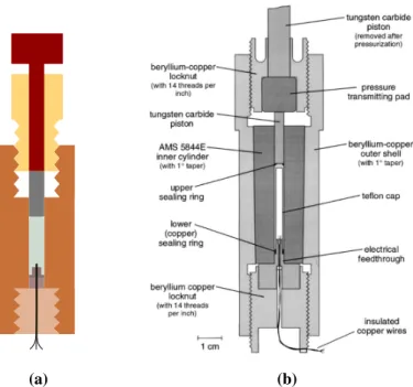
2.4 Pressure cell . . . 30

2.5 TEP pressure setup . . . 33

2.6 TEP realistic pressure setup . . . 34

2.7 TEP side view of pressure setup . . . 34

2.8 Toulouse sample holder . . . 36

3.1 Phase diagram of Nd-LSCO . . . 38

3.2 Signature of CDW and Pseudogap in Hall effect in Nd-LSCO . . . 39

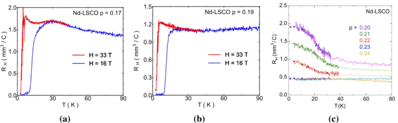
3.3 Resistivity field sweeps in Nd-LSCO p = 0.17,0.19 . . . 40

3.4 Hall effect field sweeps in Nd-LSCO p = 0.17,0.19 . . . 40 xiii

3.5 Normal state resistivity in Nd-LSCO p = 0.17,0.19 . . . 41

3.6 Normal state Hall effect in Nd-LSCO p = 0.17,0.19 . . . 42

3.7 Resistivity vs temperature in Nd-LSCO . . . 42

3.8 Temperature dependence of resistivity and Hall effect in Nd-LSCO at p = 0.15 43 3.9 Doping dependence of Hall coefficient in Nd-LSCO . . . 44

3.10 S/T vs T in Nd-LSCO and Tmaxphase diagram . . . 45

3.11 S/T vs doping in Nd-LSCO and complete phase diagram . . . 47

3.12 S/T vs doping in Nd-LSCO and complete phase diagram . . . 48

3.13 Hall effect under pressure in Nd-LSCO p = 0.12,0.15 . . . 49

3.14 Hall effect vs T in Nd-LSCO p = 0.12 at different fields . . . 50

3.15 Hall effect vs T in Nd-LSCO p = 0.12 at 16,18T . . . 50

3.16 Resistivity vs T in Nd-LSCO p = 0.12 at different fields . . . 51

3.17 Seebeck coefficient over T vs T in Nd-LSCO p = 0.12 at different fields and pressures . . . 52

3.18 Seebeck coefficient over T vs T in Nd-LSCO at p = 0.12, H = 18T and at different pressures . . . 53

3.19 Characteristic temperatures vs pressure in Nd-LSCO p = 0.12 . . . 53

3.20 Temperature dependence of the Hall coefficient in Nd-LSCO, LSCO and YBCO . . . 54

3.21 Resistivity of Nd-LSCO p = 0.17 under pressure at H = 0T . . . 55

3.22 Resistivity and Seebeck effect of Nd-LSCO p = 0.17 under pressure at H = 18T . . . 55

3.23 Resistivity vs T in Nd-LSCO at p = 0.17 at high magnetic fields . . . 56

3.24 Hall effect of Nd-LSCO p = 0.17 under pressure at H = 18T . . . 56

3.25 a)Hall coefficient as a function of temperature in Nd-LSCO p = 0.17 under pressure at high fields . . . 57

3.26 Phase diagram and correlation between p* and p_FS . . . 58

3.27 Pressure effect on the onset of pseudogap . . . 59

3.28 Effect of pressure on Nd-LSCO. . . 60

3.29 Effect of doping and pressure on Nd-LSCO. . . 61

3.30 Effect of pressure on the Hall coefficient of Nd-LSCO at p > p*. . . 62

3.31 Effect of pressure on p* . . . 63

3.32 Field dependence of Seebeck coefficient under pressure at p = 0.22,0.24 . . 65

3.33 Field dependence of Nernst coefficient under pressure at p = 0.22 . . . 66

3.34 Field dependence of Nernst coefficient over T under pressure at p = 0.24 . . 67

3.35 Effect of pressure on Seebeck and Nernst coefficient . . . 67

3.36 S/T vs log(T) for Nd-LSCO at p = 0.22 and 0.24 under pressure . . . 68

3.37 Field dependence of resistivity in Nd-LSCO p = 0.24 . . . 71

3.38 Subtraction of resistivity in linear and quadratic fit for Nd-LSCO p = 0.24 . 72 3.39 Field dependence of resistivity in Nd-LSCO p = 0.24 . . . 73

3.40 Temperature dependence of resistivity in Nd-LSCO p = 0.24 . . . 74 3.41 Field dependence of resistivity in LSCO p = 0.24 at 50-84 T of fit interval . 75

3.42 Residual of resistivity of linear and quadratic fits in LSCO p = 0.24 . . . 77 3.43 Temperature dependence of resistivity in LSCO at p = 0.24 . . . 78 3.44 Field dependence of resistivity in LSCO p = 0.19 and 0.24 . . . 79 3.45 Subtraction of resistivity in linear and quadratic fit for LSCO p = 0.19 and 0.24 80 3.46 Scaling mechanism check for Nd-LSCO and LSCO at p = 0.24 . . . 81 3.47 Scaling in LSCO p = 0.18 . . . 81 3.48 Summary of my results on the Nd-LSCO phase diagram . . . 84 A.1 Hall effect as a function of temperature in zero and in 1.7 GPa in Nd-LSCO

p = 0.15 . . . 88 B.1 Temperature dependence of resistivity in Eu-LSCO at different pressures . . 90 B.2 Resistivity as a function of logarithm of resistivity in Eu-LSCO p = 0.08 . . 90 B.3 Temperature dependence of resistivity in LSCO p = 0.06 at different pressures 91 B.4 Resistivity as a function of logarithm of resistivity in LSCO p = 0.06 . . . . 92 C.1 Temperature dependence of thermal conductivity over temperature in

Nd-LSCO at p = 0.17 . . . 94 C.2 Temperature dependence of thermal conductivity over temperature in

Literature review on transport

properties and the effect of pressure

in cuprates

Superconductivity is one of the most cutting-edge and influential fields of physics. Research on superconductivity provided insights in many other fields of physics. It was provided the first conjecture of a self-interacting boson field [1] that was later used in the Higgs mechanism and the theoretical development of many body systems. It is also an accessible example of collective phenomena and holographic duality [2]. In physics, we are mostly dealing with approximations and imperfect phenomena, but superconductors have been proven to be perfect conductors with absolute zero resistance1.

Superconductivity is an emergent phenomenon which appears when the mobile electrons of material form a collective and coherent state. The electronic correlations inside the superconductors become stronger by increasing the lattice complexity (which happens by increasing the number of distinct constituents of a superconductor material).

Superconductors already have many applications in industry and scientific research, for instance as a superconductor material can pass a significant current density when it is in the form of a wire. It can also produce a large magnetic field which is in high demand for particle accelerators like CERN or Magnetic Resonance Imaging (MRI). However, it is foreseen that the significant direct impacts of superconductivity to human civilization are yet to come! The discovery of room temperature superconductors or the economic and efficient means of cooling could have a comparable impact to the discovery of transistors and even conductors themselves. This breakthrough could have possible applications ranging from the electronics industry to transportation and space exploration.

1_{A group of researchers measured zero resistivity in the superconducting state for two and half years [3].}

In this chapter, we discuss basic concepts that are being used to explain the mechanisms of superconductivity and related phases close to the superconducting state.

There are two types of superconductors. Type I consists of about 20 elements where the magnetic field remains zero inside it until superconductivity is suppressed by critical field Hc and type II are compounds of two or more elements2. In the latter type, the magnetic

field can partially penetrate inside the superconductor in fields higher than the lower critical fieldH_c1 but the superconductivity gets suppressed only above the upper critical fieldHc2

and, in between, a vortex state exists in the material while it is in the superconducting state. Throughout this thesis, only type II superconductors are discussed. Among the type II superconductors, there are two categories: conventional and unconventional ones. The former type is a kind of superconductor which could be explained by the BCS theory with electron-photon pairing [4] and its maximumTc is typically less than 30 K3[6]. The latter

type is the one which cannot be explained by that theory.

A superconductor should have two distinct characteristics. First, its resistivity should go to zero at certain temperatures—Tc— and remains zeroT <Tc. Second, it should be a

perfect diamagnet that is shown by M=–H where H is the applied magnetic field and M is the magnetization of a superconductor in the presence of H.

The normal state of a type II superconductor can be reached above the upper critical field H_c2. We are interested in studying the normal state, and our approach is to apply a sufficiently high magnetic field to suppress the superconductivity. For the material that we mostly study here, La_1.6−xNd0.4SrxCuO4, we can reach the normal state down to the low

temperature at all dopings by applying 30T or less.

1.1

Cuprate superconductors

Cuprate superconductors (we also refer to it as cuprates) are layered materials consist of CuO2superconducting planes with stacks of other atoms. According to scholarly indexing

websites, cuprates are the branch of condensed matter physics that are most cited after semiconductors and this field is still popular as there are different phases near superconduc-tivity that have yet to be explained. It is ironic that the best-understood phase in cuprate superconductors is the superconductivity itself! The hottest debates are evolving around the other phases such as pseudogap, spin and charge density wave, strange metal and their interplay.

2_{Except Niobium, Vanadium and Technetium.} 3_{Although in 2015, H}

3—a BCS superconductor— became superconductor under pressure withTc= 203

Temperatur e Doping FL p* Tc T* PG SDW AF CDW

Figure 1.1 Sketch of the general phase diagram of cuprate superconductors. This diagram presents temperature and doping dependence of different phases of cuprates. Starting from the left side of the phase diagram, at p = 0 the material is a Mott insulator. By going to the right side, the percentage of doping is increasing. The dark red region is an Antiferromagnetic phase (AF). The boundary of the AF phase denoted by a black line represents Néel transition temperature. Spin density wave (SDW) is shown by medium red colour and charge density wave phase is coloured gray. The pseudogap phase is shown by the light red colour and its boundary with the strange metal region (white regions) is called the pseudogap temperature onset (T*) and it ends at critical doping (p*). The superconductivity dome is denoted by dashed black line. Fermi liquid phase is denoted by the light blue shades. Courtesy of Francis Laliberté.

1.1.1

Phase diagram and evolution of Fermi surface with

dop-ing

Fig 1.1 shows a general sketch of the phase diagram of the cuprates (for the interest of generalizing this sketch for all the cuprates, the y and x-axes have arbitrary units and scales). The undoped material is a Mott insulator [7] where electrons are well-localized because of a strong on-site repulsion. As one dopes the material with holes and removes some electrons from the CuO₂planes, the electrons become less restrained to move (as the Coulomb repulsion is reduced). However, at low dopings and low temperatures the material still remains an insulator, but by increasing the doping it losses its insulating properties eventually (usually above the hole content of p = 0.08).

Fig 1.1 shows the antiferromagnetic phase (AF) with the boundary of the Néel transition temperature. After that, there is another phase in which a magnetic order has been seen, this phase is known as spin density wave (SDW). The endpoint (p_SDW) is material-dependent.

0 50 100 150 200 250 0 0.05 0.1 0.15 0.2 0.25 0.3 T_c -LSCO Nd/Eu T_ν T_ρ ARPES T* T ( K ) p

Figure 1.2 Phase diagram of Nd-LSCO (red), Eu-LSCO (green) and LSCO (black). Tρ(circles) and

Tν(squares) are showing pseudogap onset T* probed by resistivity and Nernst effect respectively [8].

ARPES measurement that observed opening of pseudogap is denoted by squares[9].

For example pSDW =0.08 in YBCO [10] and pSDW =0.13 in LSCO.[11]. This phase is

believed to compete with the superconductivity phase [12].

Another short-range order like SDW is charge density wave (CDW) which is denoted by grey in Fig 1.1. There are various studies concerning the symmetry and commensurability of CDW, SDW and the mixture of the two in the cuprates [13, 14, 15]. It was believed that CDW is always observable at higher temperatures compared to SDW order (which is generally true atp =0.12, but not at other dopings). Thus, CDW is a prerequisite to SDW in a stripe phase and the stripe-order transition should be charge driven [16, 17].

All of these phases with short-range order are located inside a much bigger phase: the pseudogap phase. The pseudogap phase and its origin are the most mysterious part of the cuprates so far! It is stronger in the lower dopings and for some cuprates, it abruptly disappears at the doping level referred to as p* (shown in Fig 1.1 with a red circle). T* is the boundary between this phase and the strange metal phase (white shaded region). T* is thought to be a crossover which makes it hard to pin down (as opposed to a phase transition which is easier to observe). The superconducting dome ends at the heavily overdoped region above which there is a Fermi liquid phase that is denoted by blue colour. We call the dopings above the optimal doping—whereTc is highest— overdoped and the dopings below that as

underdoped.

In the interest of brevity, we focus primarily on the CDW and pseudogap phases al-though the Fermi surface of all of the mentioned phases is discussed briefly. Here we study the La2−xSrxCuO4 (LSCO) family of superconductors and almost all the focus is

a

b

c

p*

p

d

Figure 1.3 Sketch of the Fermi surface in different phases of cuprates. From left to right the doping is increasing. a) Electron pockets of the reconstructed Fermi surface by CDW. b) Fermi arcs that are gapped out by the pseudogap. When pseudogap is bigger and stronger, the Fermi arcs are smaller, and they are located on the antinodal region. c) Big hole-like Fermi surface above the pseudogap critical point p*. d) Above pFSthe Fermi surface goes through the Lifshitz transition and becomes

electron-like. SDW phase is located below and even inside the CDW. There is a small region between SDW and AFM where there is only superconductivity and pseudogap.

on La_1.6−xNd0.4SrxCuO4, labelled as Nd-LSCO hereafter, although La1.8−xEu0.2SrxCuO4

(Eu-LSCO) is in this family and sometimes recalled for comparison. In Nd-LSCO, the doping content is changed by varying the strontium content (x).

Figure 1.2 shows the phase diagram of LSCO family superconductors: T* was deter-mined either by resistivity or via Nernst effect as discussed below and both of these results are in agreement with the ARPES measurements (all the data are obtained from [8] and the references therein).

Fig 1.3 shows the evolution of the Fermi surface in the hole-doped cuprates. Starting from overdoped part of the phase diagram, the Fermi surface consists of a large hole-like cylinder Fig 1.3-c, as seen in Tl-2201 [18]. This hole-like cylinder continues to grow up until the Fermi surface goes through the Lifshitz transition at p_FS. It happens at the hot spots where the two large hole-like cylinders touch one another and the Fermi surface becomes electron-like [19] (fig 1.3-d). This electron-like Fermi surface is located inside the antiferromagnetic zone boundaries (dashed line in Fig 1.3-d). Below p*, due to the presence of the pseudogap, some parts of the Fermi surface are gapped out leaving Fermi arcs as shown in Fig 1.3-b. The size of the Fermi arcs depends on the strength of the pseudogap; when the pseudogap is stronger, it can gap out a larger portion of the Fermi surface resulting in smaller Fermi arcs. The pseudogap is more dominant on the Fermi surface at lower dopings and temperatures as seen by STM [20].

Fig 1.3-a shows the reconstructed Fermi surface which is the result of the transformation of these Fermi arcs into the electron pockets by CDW order. These nodal electron pockets are detected by quantum oscillations [21, 22] in YBCO.

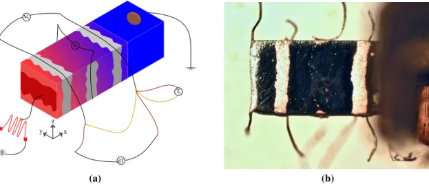
a)

b)

Figure 1.4 a)Transverse neutron scattering scans through Q = (2+2ϵ,0,0) in Nd-LSCO p = 0.12 which corresponds to the CDW peak for temperatures as indicated. The data are obtained from Ref [23]. b) Temperature dependence of lattice peak intensities for Nd-LSCOp=0.12 normalized at T = 11K. Circles are the peak intensity that have magnetic origin, squares have CDW origin and triangles are showing the structural transition from LTT to LTO. The data are obtained from Ref [13].

1.1.2

Charge order

A redistribution of electron density in the copper-oxide planes causes the appearance of a periodic charge structure called charge order, which is also known as charge density wave (CDW).

CDW was observed in Nd-LSCO by neutron scattering [13, 23] and also in other cuprates such as YBCO with resonant x-ray scattering [25], resonant soft x-ray scattering [26], x-ray diffraction [27] and with the NMR technique [28] and [29].

Fig 1.4-a shows the peak intensity obtained by neutron scattering [23] through Q = (2+2ϵ,0,0), where ϵ≈p≈0.118, which corresponds to the presence of charge density wave in Nd-LSCO at p = 0.12. The intensity of this peak increases as temperature decreases showing that the strength of CDW rises.

Fig 1.4-b shows the temperature dependence of integrated peak intensities of the super-lattice. The abrupt drop is due to the structural transition from low-temperature tetragonal (LTT) at lower temperatures to low-temperature orthorhombic (LTO) at higher temperatures. The peak that is associated with LTT is not observable when the structure is LTO. The other two peaks corresponding to magnetic and charge order. The peak at Q = (0,2-2ϵ,0) is associated with charge density wave order and at Q = (1/2,1/2−ϵ,0) is related to a magnetic

a)

b)

Figure 1.5 a- Real space mapping of charge order intensity in copper-oxide plane of Bi-2212 and NaCCOC along Cu and Ox direction that is denoted by solid and dashed arrows respectively. b- Left:

Cartoon of the charge intensity map in the copper-oxide plane with the maximum intensity located at Oxand Q = (0.25,0). The Figures are obtained from the Ref [24].

coexist, they called stipe order. The magnetic order in Nd-LSCO is similar to the CDW phase as the periodicity of their modulations is commensurate and they lock inside each other. The spin density wave is related to a change in the distribution of spins and the creation of periodic modulated magnetic structures. Fig 1.4-b also shows that the onset of CDW and SDW are different and their intensities increase at lower temperatures.

In the cuprates and in more complicated cases, the CDW modulations could be biaxial or unidirectional which are the consequence of different wave vectors that reconstruct the Fermi surface and it is material dependent [30, 31]. CDW modulations have been detected directly by Scanning Tunneling Microscopy (STM) measurements, thereby showing charge order in some other cuprates; notably the Bi₂Sr₂Ca Cu₂O₈+xBi-2212 and Ca2−xNaxCuO2Cl2

(NaCCOC) systems, as shown in Fig 1.5. Fig 1.5-a shows the real space map of charge modulations on Cu and Oxsites denoted by solid and dashed arrows respectively. Fig 1.5-b

shows a cartoon of the d-form factor density wave and shows that their periodicity is 4 lattice constants. In another words Q = (0.25,0). On the right side of this cartoon the calculated CDW scheme is shown from this d-form factor density wave model.

It is essential to study the CDW phase as it appears to have competition with the superconducting phase. In particular, its presence causes a dip in the superconducting dome [32]. Another signature of CDW is the presence of a dip in H_c2 vs p [33] measured by thermal conductivity. Furthermore, some theories suggest the pseudogap and CDW have the same critical point and they end at the same doping of p* [34, 16, 35].

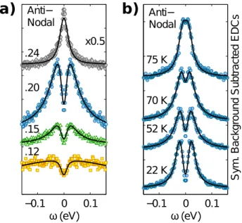
−0.1 0 0.1 ω (eV) .24 .15 .20 .12 x0.5 (h) Anti− Nodal −0.1 0 0.1 ω (eV) 22 K 52 K 70 K 75 K S ym . B ac kg ro un d S ub tr ac te d E D C s Anti− Nodal (l)

b)

a)

Figure 1.6 a) Energy distribution curves of Nd-LSCO in different dopings at temperatures right above theTc. The curve at p=0.24 (gray) is above the pseudogap and the rest of the curves are in

the pseudogap at p < p*. b) Energy distribution curve for Nd-LSCO p = 0.20 at different temperatures. All the curves are arbitrary shifted vertically for clarity and symmetrized. The Figure is obtained from Ref[9].

Around p=0.125, there is a dip in the superconducting dome as shown in Fig 1.2. As the charge order phase is located around this doping range, it is thought that it competes with superconductivity and is responsible for loweringTc. One way to investigate that, is

to suppress this order by the application of pressure. This has been done in YBCO and by suppressing the CDW via pressure [32, 36], the dip in the Tc dome was removed and the

full shape of the dome was recovered, meaning that there is indeed a competition between CDW and superconductivity in this system. We verified the possibility of CDW suppression by pressure in Nd-LSCO and we discuss it further in chapter three.

1.1.3

Pseudogap phase

The pseudogap was discovered via the NMR technique in less than three years after the discovery of superconductivity in the cuprates [37, 38]. It is currently the central puzzle of the cuprate superconductors, and different theoretical and experimental groups are trying to delineate the relationship between the pseudogap and other phases with different approaches (e.g. by suppression of the density of states).

The onset of the pseudogap in temperature is represented by T* and the endpoint of the pseudogap in doping is known as p* (the doping at which T* goes to zero), both of which

have signatures in transport probes as well as spectroscopic measurements. We discuss its transport signatures later on in this chapter. By using angle-resolved photoemission electron spectroscopy, ARPES, one can find spectroscopic evidence of this phase [39, 40, 41, 42].

Fig 1.6-a, shows symmetrized energy-distribution curves for several dopings of Nd-LSCO at temperatures just aboveTc. A gap (manifested by a drop in the spectral weight at

ω = 0 eV) in the anti-nodal region appears at dopings 0.12, 0.15 and 0.20, but at p =0.24

it disappears. The presence of this gap means that the density of states decreases and is associated with the pseudogap. Hence, one can conclude that the pseudogap closes between p = 0.20 and 0.24 [9]. In Nd-LSCO, by tracking the signatures of resistivity and Hall effect, the pseudogap endpoint was pinned at p* = 0.23±0.01 [43].

The pseudogap phase also has a signature in temperature. Fig 1.6-b, shows the spectral weight in the anti-nodal direction for Nd-LSCO at p = 0.20<p*. At 75K there is no gap in the spectrum. By decreasing the temperature, a gap opens up and becomes bigger down to 22K (which is still aboveTc).

In Fig 1.2, if one extrapolates the T* line up to the overdoped region, it ends at the end of the superconductivity dome which suggests that the same interactions might be responsible for the pseudogap and superconductivity (nevertheless, the pseudogap suddenly disappears at p*). The left side of the T* line at the zero doping intercepts the onset of the Néel temperature (fig 1.1) which provides support for the antiferromagnetic origin of the pseudogap. Spin modulations (spin density wave or SDW) have been detected right after the AFM phase(Fig 1.1), hence their origin might be the same as the AFM phase, even though the SDW modulations are short-range. The endpoint of the SDW phase is thought to be located at p* [11] (experimental evidence is required here, but the fact that SDW phase is still present after the endpoint of the CDW phase and before p*, as in Nd-LSCO, supports this hypothesis) which again promotes the AFM origin of the pseudogap phase.

Later on in this chapter, we focus on the signatures of the pseudogap in the transport experiments and discuss some of these theories but the pseudogap is a highly debated phase and it is not evident if it is a friend or foe or a friendly foe of the superconductivity and the other phases in cuprates [34].

1.1.4

Fermi Liquid and strange metals

In Fermi-Dirac statistics, conduction electrons in a metal are treated as non-interacting fermions in a Fermi gas and the system is called Fermi liquid. Based on the Pauli exclusion principle, electrons at the Fermi surface are only allowed to have a sort of collision that can change their momentum with the assumption of a one-one condition (there is no interaction between many electrons simultaneously). In the low temperature limit where the one-one condition holds, the interactions are renormalized the parameters like the effective mass

(m∗) which gives the T2resistivity and the specific heat becomes linear in temperature as the resistiv

In the marginal Fermi liquid theory [44] this assumption has been modified so that it can explain other transport signatures that could not be explained with Fermi liquid theory. Some theories suggest that the superconductivity in cuprates is born from the over-doped side of the phase diagram where the Fermi liquid regime starts to break [7]. Between the Fermi liquid phase and the pseudogap in high-temperature superconductors, there is a phase called strange metal that is the consequence of this ”alteration” or ”break down” of Fermi liquid regime. In this system, one should consider the collective interaction of electrons together (instead of just taking the one-one condition into account) in order to explain the deviation from the T2resistivity of the Fermi liquid regime.

In a temperature range above T* for p = 0<p<p* and at T→0 for p* <pc 4, the

normal state resistivity in the cuprates has a linear temperature dependence, which can not be explained by the conventional theory of metals. It has been shown recently, both in the hole and electron-doped cuprates, that regardless of the governing inelastic scattering mechanisms, whenever the scattering rate (1/τ) reached its Planckian limit 1 / τ = kB T /

¯h the resistivity becomes T-linear [45]. It is why this region in the phase diagram is called ”Strange Metal”.

The temperature dependence of the resistivity at p>p_c has the form of Tα _{where 1 < α}

< 2 [46]. On top of that, the AC conductivity has a frequency dependence [47] which is also incompatible with the conventional theory of metals. Besides, through the suppression of superconductivity at the dopings in the vicinity of p*, the residual resistivity has a linear field dependance [48] which has not yet been explained.

To study this phase of cuprates, we looked at the temperature and field dependence of resistivity that is discussed in the last part of chapter 3.

1.2

Electrical transport properties

1.2.1

Resistivity

Resistivity is a measure of scattering of electrons in the lattice. At T = 0, the dominant mechanism for scattering is due to all possible kinds of impurities and imperfections in the crystal such as vacancies, interstitials, and dislocations. At T > 0 K, other scattering mechanisms (such as electron-phonon inelastic scattering) come into play. We use the Drude

(a) (b)

Figure 1.7 a) Temperature dependence of resistivity at p = 0.22 < p* = 0.23 in Nd-LSCO. Dashed black line shows linear fit of resistivity in either zero magnetic fields or H = 16T and the point that resistivity deviates from linear fit is shown with arrow [43] b) Temperature dependence of resistivity at different dopings, different colours showing different doping and same colour code used for arrows to show T* [43]. All Figures present the in-plane resistivity.

formula to interpret resistivity ρ = m/ne2τ, where τ is the scattering rate, m and e are the

mass and electric charge of electron respectively and n is the density of electrons.

More than two decades ago it was discovered that the temperature dependence of resistivity deviates from linearity [49]. The point below which resistivity is not linear and it shows either a downturn in YBCO [49] or an upturn in Nd-LSCO [49] is known as the onset of the pseudogap—T*. Here we only focus on the upturn of pseudogap for Nd-LSCO. Resistivity depends on the number of carriers and scattering (elastic and inelastic). When the pseudogap appears, the density of states, the carrier density and the inelastic scattering all decrease (and the decrease in the magnitude of one may or may not be the consequence of a decrease in another). In a clean system such as YBCO, when the pseudogap opens, as the dominant source of scattering is the elastic scattering, the inelastic scattering decreases which results in a decrease in resistivity. But in a dirty system like Nd-LSCO, when the pseudogap, the inelastic scattering does not change that much as it is dominant, so, as there are fewer carriers in the system, the resistivity rises.

In Fig 1.7-b T* is shown for different dopings of Nd-LSCO by different arrows. At the dopings above the pseudogap p* < p, there is no T* and the resistivity presents no upturn related to the pseudogap as shown in Nd-LSCO atp =0.24 in Fig 1.7-b, where ρ remains T-linear down to T→0.

4_p

(a) (b) (c)

Figure 1.8 Comparison of LSCO (red) and YBCO (green) atp=0.12 a)X-ray intensity as a function of temperature associated with the CDW modulations, normalized atTc, detected in LSCO [50] and

YBCO [27], the peak is atTc. b) Temperature dependence of Seebeck coefficient over temperature

measured in YBCO [51] and LSCO [52] in the presence of magnetic field (normal state) c)Hall effect of YBCO at 15T [53, 54] and of LSCO at 16T [52].

1.2.2

Hall Effect

In the simplest model of an isotropic Fermi surface,RH is the Hall number that is calculated

as RH ≈ ±1/ne, where n is the number of carriers per unit volume and e is the electron

charge. The carriers determine the sign ofRH, if the majority of carriers are holes the sign

ofRH is positive, otherwise it is negative. One can calculate the Hall number nH

nH =

V RHe

(1.1)

where V is the unit cell volume.

The effect of CDW in LSCO and YBCO is a clear drop in Hall coefficient [52]. Fig 1.8-a shows the intensity of X-ray vs temperature for LSCO and YBCO. The temperature at which the intensity is increasing is related to the onset of CDW.

It should be mentioned that the superconductivity could cause a downturn as well, but the difference is that it must happen nearTc and it is much more abrupt compared to

the downturn that signifies CDW. This makes observing CDW hard for transport probes, especially whenTCDW is located near or even belowTc. In this case, one needs to suppress

superconductivity and consequently the downturn that corresponds to it; to be able to locate TCDW. We do this through the application of high magnetic fields.5We argue that when we

5_{One must notice that the magnetic field is being used only to suppress the superconductivity. Also, it does}

not have any effect on the CDW. One must notice that the CDW phase is not field-induced or field dependent. As the drop in the Hall coefficient vs T does not change at different fields (at least for a considerable range of temperature) both above and below theTc.

apply the magnetic field on dopings for whichTcis well-separated fromTCDW, the magnetic

field cannot moveTCDW at all.

Positive and negative curvatures of the Fermi surface cause hole and electron-like Hall response as discussed in Ref [57] (the interpretation of the Fermi surface geometry on the Hall coefficient is obtained by using the conventional Boltzmann theory). However, when the Fermi surface has both a positive and negative curvatures the Hall response is the balance between the hole and electron-like contributions of the Fermi surface [58]. Thus, Hall effect can reveal any phase that reconstructs the Fermi surface and changes its geometry, but one should be aware of the complications behind the Hall signal (e.g., the presence of positive and negative curvatures both in a single Fermi surface and in a multi-band system). In cuprates superconductors at the CDW phase, the drop inRH vs T marks the onset temperature at

which Fermi surface starts to get reconstructed by CDW.

Pseudogap also has a signature in Hall effect. In Fig 1.9-a, temperature dependence of Hall effect is shown in Nd-LSCO for several dopings; at p < p*, there is an upturn as was the case for resistivity.

In Nd-LSCO, by obtaining the Hall coefficient at low temperature and in high magnetic fields and knowing that V/e in this material is 0.625 m3/C (as in LSCO), one can calculate the normal state Hall number, n_H. Fig 1.10 shows the trace of Hall number for two completely different materials at different dopings. It is shown that there is a drop in carrier density from 1+p to p as the doping drops below the p*. Having 1+p carrier density means that the Fermi surface is hole-like (a large hole like Fermi surface has been seen in Tl-2201 [18] by ARPES). In an antiferromagnetic scenario, this large Fermi surface folds and makes nodal hole pockets and antinodal electron pockets in the drop between 1+p to p. However, the nature of Fermi surface reconstruction at p* is not yet known.

1.3

Thermoelectric transport properties

Thermoelectric coefficients are also sensitive to the band structure. In all of the thermoelectric measurements that are mentioned in this thesis, the magnetic field is applied along the c-axis, a longitudinal thermal gradient is applied within the CuO2planes and a Seebeck or Nernst

voltage in the a-b plane has been measured. The schematic of our experimental setup is discussed in chapter two.

(a) 0 50 100 150 200 T (K) 0.0 0.5 1.0 1.5 2.0 2.5 3.0 RH (mm 3C –1) YBCO p =0.16 0.177 0.19 0.205 b (b) 10 30 50 70 90 H ( T ) 0.0 0.5 1.0 1.5 2.0 2.5 RH (mm 3C –1) YBCO T = 50 K p =0.16 0.177 0.19 0.205 (c)

Figure 1.9 a) Temperature dependence of Hall coefficient at the dopings below and above p* in Nd-LSCO in low (light colour) and high magnetic field of 33T (dark colours) [43] b) Back extrapolation of Hall coefficient vs temperature in YBCO in high magnetic fields up to 80T, circles are field sweep cuts that are shown in plot (c) [52]. At p = 0.205 which is located above p*, there is no upturn that is the characteristic of pseudogap. c) Field dependence of Hall coefficient in YBCO. Compared to Nd-LSCO, YBCO requires higher magnetic fields for the suppression of superconductivity needed to revealRH(0) [52].

Figure 1.10 Doping dependence of Hall number nHis shown for Nd-LSCO (red squares) and YBCO

(blue circles). In low dopings the gray squares are Hall number in LSCO [55] and gray circles are for YBCO [56]. Solid lines are guide to the eye and p* at 0.195±0.01 and 0.23±0.01 for YBCO and Nd-LSCO respectively. The Figure is obtained from the Ref [43].

Figure 1.11 Seebeck coefficient over T as a function of temperature in different superconductors at p=0.12 (1/8 anomaly) data and Figure obtained from Ref [59] and references therein.

1.3.1

Seebeck Effect

We obtain the Seebeck coefficient,S, via S = VS

dTx, whereVS is the longitudinal Seebeck

voltage anddTx is the longitudinal temperature difference (the detailed discussion on how

we measure the Seebeck effect is mentioned in the second chapter). Like the Hall effect, the Seebeck coefficient can determine the sign of the majority of carriers. The balance between the electrons and holes that are moving in the thermal gradient can determine the sign of the carriers. The difference with the Hall effect is that in this case, it is not necessary to apply a magnetic field.

As shown in Fig 1.8-b, CDW has an effect on the Seebeck coefficient that is similar to its effect on the Hall coefficient (RH). Fig 1.11 shows the Seebeck effect in different

materials at p=0.12 which is also known as the 1/8 anomaly.

In summary, charge density wave modulations cause a Fermi surface reconstruction [60] which has a clear signature in our transport probes.

1.3.2

Nernst Effect

In the presence of an applied magnetic field, a thermal gradient inside a conductor, that does not have any net electrical current flowing inside it, can produce a transverse voltage that is

YBCO p = 0.078 p = 0.085 T T / T ( nV / K 2 T ) T ( K ) -0.05 0 0.05 160 180 200 220 240 260 280 300 (a) Nd-LSCO p = 0.20 p = 0.24 T_c T / T ( nV / K 2 T ) T ( K ) -0.4 -0.2 0 0 20 40 60 80 100 120 140 -0.4 -0.2 0 (b)

Figure 1.12 Temperature dependence of Nernst coefficient over temperature for a) highly under-doped YBCO at two dopings and b) in Nd-LSCO at p = 0.20 (red) andp=0.24 which are below and above the pseudogap respectively. Tν marks the onset of pseudogap, T*. Figure obtained from Ref [8].

called the Nernst voltage, N, and is calculated as:

N= −Ey ∇Tx

(1.2)

The Nernst coefficient is ν = N/H where H is the magnetic field. In the T = 0 limit, it has approximately the following magnitude:

ν= π 2 3 kB e kBT EF µ (1.3)

Where E_F is Fermi energy and µ is mobility, which means that the Nernst coefficient is determined by the Fermi energy and mobility. There are three physical phenomena that could contribute to this signal which are quasi-particles, superconducting fluctuations and superconducting vortices [61]. Again, we will suppress the latter two contributions by applying a large field. In two dimensions, the magnitude of the Nernst coefficient is inversely proportional to the carrier density, as in low carrier densities the Fermi energy is lower. Here we plot ν over T instead of ν.

To delineate the pseudogap more precisely, one can use the Nernst effect. Fig 1.12 shows the temperature dependence of the Nernst coefficient as a function of temperature for YBCO and Nd-LSCO. Tνis the temperature at which ν/T deviates from linearity which coincides

-0.1 0 0 50 100 150 200 250 300 Eu-LSCO / T ( nV / K 2 T ) T ( K ) 0.08 0.10 0.125 0.16 0.21 -0.2 0 LSCO 0.05 0.07 0.125 0.15 0.17 -0.4 -0.2 0 Nd-LSCO 0.15 0.20 0.24 (a) 0 100 200 3 6 9 12 0 100 200 300 3 6 9 12 ( nV / K T ) 30K 35K 40K 50K 60K 0 100 200 300 3 6 9 12 LSCO x = 0.07 0.10 0.12 (a) (b) (c) H ( T ) (b)

Figure 1.13 a) Temperature dependence of ν/T in LSCO family superconductors at different dopings. b) Magnetic field dependence of Nernst coefficient in LSCO at different dopings. Note that at high temperatures the Nernst coefficient becomes more field dependent. Obtained from [8]

with T* measured by resistivity and the pseudogap onset that is determined by ARPES, so T_ν= T* [8]. It is important to notice that it is much more straightforward to determine T* via the Nernst coefficient compared to the resistivity, as it is shown in Fig 1.13-a, the deviation from linearity below p* is much more pronounced in the Nernst coefficient as compared to the resistivity, regardless of the type of material. In Fig 1.13-b the field dependence of the Nernst signal in underdoped Nd-LSCO is shown.

1.4

Crystal structure and pressure effect

The effect of pressure on Hg-1223 [62] was to increase the Tc up to 164K and this increase

of the Tc saturates above 16GPa, which inspired many advances in the superconducting

research at that time6. In general, pressure squeezes the lattice in the real space, and that may tune the band structure too, by doing so, it can affect the transport properties of materials. Depending on the material and the magnitude of pressure, this effect might be dramatic or not. One of the motivations behind the study of the effect of pressure in cuprates is to study the phases that are competing or contributing to superconductivity and to demystify the nature of those phases too. Here we only mention the related pressure effect on our material of interest Nd-LSCO.

CDW modulations in LSCO itself have been studied and are found to cause distortion in the CuO2planes near the doping of p =0.12 which is thought to be the source of 1-D

modulations [63]. Observing the structure of CuO6octahedra in this material could be useful

for understanding this phase. In this material, two different simultaneous modulations have been detected. In Fig 1.14 the two different kinds of octahedron structures that give rise to these different stripe modulations are shown. The Cu sites form stripes of the distorted lattice (D-stripes), that are intercalated by the stripes of an undistorted lattice (U-stripes). Moreover, the LTT (low temperature tetragonal) type of distorted CuO6octahedra is assigned to the

D-stripes and the U-D-stripes are assigned to the LTO (low temperature orthorhombic) structure. As LSCO is the strongest material (its lattice is less susceptible to deform by the application of pressure) in Lanthanum family of superconductors [66], the effect of pressure should not be highly noticeable in it. So to check the effect of pressure in stripe or charge order, we turn to LBCO, that is the first cuprate that was discovered [67], which is both close to Nd-LSCO structure-wise and is in the same family of Lanthanum superconductors. Fig 1.15-a shows the crystal structure of LBCO. At the copper oxide plane, where the super-current passes, any sort of distortion could affect the superconductivity. Above and below that plane are two oxygen atoms that form the CuO6octahedra that are mentioned above. In Fig 1.15-b,

the configuration that gives rise to the LTO phase is depicted. The tilting angle (direction) which is a measure of the orientation of this octahedron are shown as well. In Fig 1.15-c the configuration of an octahedra which is responsible for the LTT phase is shown.

The situation is more or less the same in Nd-LSCO too. In Fig 1.15-d the CuO₆octahedra in Nd-LSCO is shown. To better categorize different structures in Nd-LSCO, one can define an order parameter called Q. It determines the tilting direction of these octahedron. The HTT rotation axes are defined as (110) and (1-10) as shown in Fig 1.15-d. If the octahedron

6_{However, the highestT}

crecord holder is sulfur hydride [5] at the moment with theTcof 203K, it is not

a cuprate though and it is the classical BCS superconductor so does not have lots of practical advantage of cuprates, for instance, its critical field at 200K is below 500Oe, on the other hand, reaching the pressure of 200GPa is extremely difficult (the pressure of the outer core of the earth is 330GPa and Iron melts at that pressure).

Figure 1.14 The CuO6 octahedron is distorted due to the stripes. In the right side the so called

D-stripe type has the form of LTT and on the left side the U-stripe type has the LTO structure specific width for each stripe is shown. This pictorial view is obtained from Ref[63].

[100]_t La,Ba [010]t [110]_t Cu O [001] HTT LTO LTT (a) (b) [110]t [100]t [010]t (c) (d)

Figure 1.15 a) Crystal structure of LBCO in HTT phase is shown. b) The LTO phase and the tilting direction is shown. c) LTT phase and its tilting direction, obtained from Ref [64]. d) octahedra structure of CuO6in Nd-LSCO, blue and black circles are showing oxygen and copper elements

respectively different axis of copper oxide plane are shown and rotation around these axis with order parameters of Q₁and Q2are shown. Depending on the rotation, sample goes through LTT, LTO 1 or

(d)

(e)

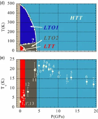
Figure 1.16 Structural phase diagram of Nd-LSCO as a function of temperature and pressure obtained by x-ray diffraction. Top: LTT phase (red) is located at low temperatures and could be suppressed by modest pressure of less than 2GPa. LTO2 (gray) and LTO1 (blue) are located above LTT and the transition between LTO2 and LTO1 fades out above 2GPa marked with a question mark. Above 4.2 GPa all the CuO6octahedron become ordered and the tilt angle→0 that cause a structural transition

to HTT. Bottom: Critical temperature of Nd-LSCOp=0.12 vs applied pressure. The colour code is the same as the top Figure. At ambient pressureTc= 3K and the highestTcis 22K at P = 5GPa in

HTT phase. Obtained from Ref [65].

rotates with respect to any of these axes in a single rotation by the magnitude of|Q₁|or

|Q₂|the LTO1 structure appears. The twin structure of LTO1 is LTO2 that is obtained by simultaneous rotations with the magnitude of Q2and Q1 around both HTT rotation axes,

provided that Q₁̸=Q₂. Finally for the formation of LTT lattice Q₁= Q₂̸=0.

The effect of pressure has been studied in Nd-LSCO at p=0.12 with x-ray diffraction [65] up to very high pressures. The top panel in Fig 1.16 shows the structural phase diagram of Nd-LSCO as a function of pressure and temperature. By increasing the pressure, the LTT phase (red) is suppressed and the structural transition from LTO2 (grey) to LTO1 (blue) increases to higher temperatures. However, the structural transition itself becomes harder to resolve (discussed in chapter 3 and denoted by a question mark in this Figure). Finally, in pressures higher than 4.2GPa, the tilt angle→0 and the structure transforms to HTT up to the highest achievable pressures. It is shown that pressure favours the orthorhombic

0 10 20 30 40 50 60 70 0.00 0.05 0.10 0.15 0.20 0.25 1.15GPa (x0.2) 2.7GPa 1.77GPa p=0GPa (x0.1) In te g ra te d I n te n si ty ( c o u n ts /s e c ) Temperature (K) 0 10 20 30 40 50 60 70 0.0 0.5 1.0 1.5 2.0 (b) (a) 2.7GPa 1.77GPa 1.15GPa p=0GPa In te n s it y ICO (c o u n ts /s e c ) Temperature (K)

(a)

(b)

Figure 1.17 a) Temperature dependence of the integrated intensity of x-ray diffraction peak at (100) which is the signature of LTT phase, by 2.7GPa this phase is fully suppressed. b) Temperature dependence of the intensity of the peak that is corresponding to charge order. Same pressure did not suppress charge order whereas it suppressed LTT phase. Obtained from Ref[68]. c) Orthorhombic strain as a function of doping. The sharp drop is a structural transition from LTT to LTO and the curve for x = 0.15 is different due to mixture of these different phases, obtained from Ref. [64].

structure (LTO2) of the lattice by reducing the tilt angle of CuO₆octahedra (fig1.16) and eventually it favours the HTT phase in pressures higher than 4GPa. The bottom of Fig 1.16 shows the evolution ofTc vs pressure.Tc from 3K increases up to 22K at 5GPa and after

that it decreases again and this drop might be due to the fact that higher pressures squeeze the c-axis.7

In this work, we study the effect of pressure on both thermoelectrical and electrical transport properties of Nd-LSCO under pressure at dopings which are located in the CDW region and at dopings around p*. Below, a few relevant studies on the nature of the pseudogap and CDW phases are mentioned.

X-ray and neutron scattering experiments have detected stripe order in the La2−xBaxCuO4

(LBCO) superconductor around the doping level of p = 0.12 [64]. It is shown that the

7_{The resistivity can reveal the structural transition in Nd-LSCO for some dopings, by showing an anomaly}

presence of these stripes is not necessarily due to the crystal structure. By suppression of the LTT structure in LBCO (that is shown by a disappearance of the (100) peak), the stripe order is not fully suppressed as shown in Fig 1.17-a. The LTT phase fades out but the CDW phase is not yet fully suppressed (In Fig 1.17-b the peak, that is the signature of charge order, partially fades out). Fig 1.17-c shows a systematic decrease of the LTO strength as a function of doping. The jumps show the LTO to LTT transition. Only at x = 0.15 the transition is a result of mixed LTO and LTT phases; the rest have sharp transitions [64]. Hence, one can conclude that the effect of pressure is the same as increasing the doping; that in both cases the intensity of LTT phase decreases. Another important conclusion is that the LTT phase is not necessary for the CDW formation.

Magnetization and muon spin rotation studies under pressure in LBCO reveal the competition between superconductivity and spin stripes and show that the pressure of 2.2 GPa can partly suppress the spin stripe modulations and reduce the magnetic volume fraction of the static stripe phase, although, they are still present after the suppression of LTT phase8 (x = 0.125) [70].

For the first time, we were able to measure thermoelectricity of cuprate superconductors under pressure and in high magnetic fields. We have developed our setup based on the following studies. Thermoelectricity under pressure has been measured in the organics [71] and more recently in pnictide family of superconductors [72]. The seebeck coefficient has been measured in YBCO and LSCO [73, 74] in a different range of doping up to 1.5GPa, but not at many different pressures. Thermoelectric power has been measured in a polycrystalline sample of Hg-1245, however in less than 1GPa [75]. The temperature dependence of the Seebeck effect in the pnictides has been studied under pressure as well [72]. The Seebeck effect under pressure is also measured in La₁−xNdxCuO3 at x = 0.5 which is close to the

Mott-Hubbard transition and is not a superconductor [76].

Electrical transport studies under pressure have been done on Nd-LSCO at p =0.12 [77], but the data are not systematic. We had a closer look at this material and investigated the effect of pressure on the adjacent and the same doping to study the competition between charge order and superconductivity by tuning the CDW with pressure.

Experimental techniques and

developments

In this chapter, the expertise that we developed to perform transport measurements under hydrostatic pressure, AC thermoelectricity measurements and high pulsed magnetic field experiments are discussed.

2.1

Transport experiments at ambient pressure

2.1.1

Resistivity and Hall Effect

Nowadays electrical transport measurements are considered to be one of the most available and conventional experimental probes. By applying the electrical current between two points and measuring the voltage drop, one can obtain resistivity based on Ohm’s law. The applied potential exerts the force of F =−eE on free electrons in a metal. Then for each electron

−eE = m (dv/dt) where m is the electron mass. If the time between the collisions, defined as

τ (Drude’s relaxation time), the electron velocity is:

ν= −eE

m τ (2.1)

B I I + _v x y z v t w l

Figure 2.1 Hall effect schematics. The deviation of electrons and holes are shown in the presence of a magnetic field. The direction of electron and hole movement is denoted by ν. The current is applied along the x-axis. The sample thickness, width and length are shown by t, l and w respectively.

The definition of current density (j), is the number of electrons with charge e that move with a certain speed in a given cross-section. Here we assume that the average electron’s speed is 2.1. Therefore j =neν= ne 2 τ m E=σ0E= E ρ0 (2.2) and the DC electrical conductivity is the inverse of ρ0which is the value that we measure1.

By measuring the Hall effect, one can obtain the mobility and sign of carriers. As shown in Fig 2.1 electrons or holes with charge -e and +e are deviated by the Lorentz force, F = qν×B, in the magnetic field that is applied upwards along the z-axis. Then with transverse contacts on the sides of the sample and along the y-axis, one can measure the voltage that is the consequence of electron or hole accumulation on one side of the sample. This voltage produces an electrical force that is in balance with the Lorentz force:

Eyq =qν×B (2.3)

where q could be±e. The Hall coefficient RH is defined as

RH = Ey jxBz = νBz neνBz = 1 ne (2.4)

and experimentally we have dimensions of the sample (length, width and thickness) and we measure transverse resistance in a given magnetic field, so R_H could be calculated in

1_{In appendix (C), there is a brief discussion on AC electrical conductivity and dependence of electrical}