HAL Id: hal-02047977
https://hal.archives-ouvertes.fr/hal-02047977
Submitted on 2 Dec 2020
HAL is a multi-disciplinary open access
archive for the deposit and dissemination of
sci-entific research documents, whether they are
pub-lished or not. The documents may come from
teaching and research institutions in France or
abroad, or from public or private research centers.
L’archive ouverte pluridisciplinaire HAL, est
destinée au dépôt et à la diffusion de documents
scientifiques de niveau recherche, publiés ou non,
émanant des établissements d’enseignement et de
recherche français ou étrangers, des laboratoires
publics ou privés.
Parameters sensitivity analysis in charge transport
model using Sobol indexes for optimization purpose
Fulbert Baudoin, Séverine Le Roy, G. Teyssedre, Laurent Crouzeix, I.
Alhossen, Florian Bugarin, Stéphane Segonds, Nicolas Binaud
To cite this version:
Fulbert Baudoin, Séverine Le Roy, G. Teyssedre, Laurent Crouzeix, I. Alhossen, et al.. Parameters
sensitivity analysis in charge transport model using Sobol indexes for optimization purpose. IEEE
International Conference on Dielectrics, 2016, Montpellier, France. �10.1109/ICD.2016.7547745�.
�hal-02047977�
(978-1-5090-2804-7/16/$31.00 ©2016 IEEE)
Parameters sensitivity analysis in charge transport
model using Sobol indexes for optimization purpose
F. Baudoin, S. Le Roy, G. Teyssedre, C. Laurent
Laplace, University of Toulouse, CNRS, INPT, UPSToulouse, France
I. Alhossen, F. Bugarin, S. Segonds, N. Binaud
University of Toulouse, UPS, INSA, ISAEICA, Toulouse, France [email protected]
Abstract— This paper aims at carrying out a parameters
sensitivity analysis on a charge transport model using an approach based on the Sobol’s method. Charge transport models generally encompass a large number of unknown or ill-defined parameters, typically 10, that interact to produce macroscopic response observable through e.g. space charge density profiles and external current measurements. However, the various physical processes of the model have different impact on the predicted behaviour. The Sobol’ approach applied herein is used to study how the variation of the current density and charges density can be quantitatively apportioned to the variation of the model input parameters.
Keywords: modelling – charge transport – Sobol indexes – LDPE material – sensitivity analysis
I. INTRODUCTION
Various physical models have been implemented for describing the mechanisms of charge generation and transport in solid dielectrics [1-3]. These models require the handling of a number of parameters like injection barrier, mobility, trapping coefficient, etc. Most of these parameters cannot be determined by independent experiments and it is a heavy task to estimate parameter values that best fit experimental data. Optimization algorithms aim at systematizing this part of the modelling activity. However, to facilitate the convergence of optimization algorithms, it is important to quantify the effect of each input variable on the output observables in order to limit the optimization to the most influential variables.
The method implemented in this work, based on Sobol's analysis, guides the choice of optimization algorithms by focussing on the main parameters affecting the charge transport model which makes the resolution possible. The task is to build a sensitivity analysis on 4 of the inputs of the charge transport models regarding the impact on the space charge density and current measurements which are the main observables that can be implemented for feeding the models. With this in hands, the optimization can select the best conditions for appropriate estimation of model parameters.
II. UNIPOLAR CHARGE TRANSPORT MODEL
A. Physical description and basic equations
The model developed here is a unipolar description of charge transport based as detailed elsewhere [1]. This model considers two levels of charge traps: a deep trap level
accounting for relatively long-lasting trapping of charges and a shallow level to which is associated an effective mobility for mobile carriers. Charge carriers have a given probability to escape from deep traps by overcoming a potential barrier that is included in the de-trapping coefficients. Two kinds of species are considered, being mobile and trapped carriers. Even when neglecting dipolar processes and diffusion one generally has to solve the following coupled equations considering a 1D problem along the spatial coordinate x, whatever the model used to describe charge transport:
) , ( . ). , ( . ) , (xt E xt en xt j µ (1) ) , ( ) , ( 1 ) , ( t x s x t x j e t t x n (2) ) , ( . ) , ( en xt x t x E (3)
where j is the transport current associated with mobile carriers of density nµ and charge e, µ is the mobility, E is the electric
field, n the total carriers density. The term s is the source term, i.e. it encompasses any local charge density variation due to processes other than transport, such as the internal generation of charges. These equations may have a specific form for the interfaces, and are complemented by boundary conditions (e.g. applied electric field, etc.). An example of an expression for the source term of Eq. 2 is given for mobile carriers:
t t t Dn n n Bn dt dn s 0 1 1 (4)
where B is the trapping coefficient, nµ and nt are respectively
mobile and trapped carrier densities, n0t is the maximal trap
density, in our case n0t is such that e.n0t =100 C.m-3. The
de-trapping probability is defined by a de-de-trapping coefficient which is of the form:
T k ew D B tr h e,
.exp . (5)where is the attempt to escape frequency, which has been set
to kBT/h = 6.2 1012 s-1 at room temperature, T is the temperature
and wtr is the de-trapping barrier. In this model, we have
supposed that charge generation results from injection at the electrodes according to a corrected Schottky law (there is no injection when the electric field at the electrode is null):
1 4 exp exp 2 electrode B B inj eE T k e T k ew AT j (6)
where jinj is the flux of charge at the electrode, kB is the
Boltzmann's constant, A=1.2 106 A.m-2.K-2 is the Richardson
constant, w is the injection barrier.
For this study, we consider low density polyethylene -LDPE material, in film form of thickness D = 200 µm, at a temperature of 40°C and under a DC electric field of 30 kV.mm-1 applied between the both electrodes during
different times of polarization: tpol of 100s, 600s and 1200s.
III. SENSITIVITY ANALYSIS
A. Model as black box
In this part, the model of charge transport described previously is viewed as a black box with some inputs and outputs that are defined as in Fig. 1.
Fig. 1. Model as a black box
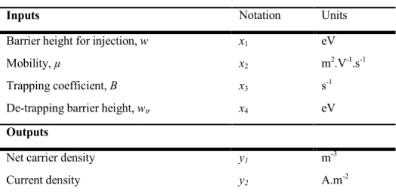
We denote input data some physical constants allowing describing the mechanisms of charge generation and transport in the solid insulation, sometimes the term parameters will be also used. In this work, only 4 inputs are considered and concern the charges injection, mobility of carriers and trapping and detrapping processes, Table I. We denote output data the main results obtained by the model. In our case, we consider only the net density of carriers and the current density because they are easily observable using experimental devices. The f function corresponds to the charge transport model described previously and includes all the partial differential equations.
TABLE I. INPUT AND OUTPUT DATA
Inputs Notation Units
Barrier height for injection, w x1 eV
Mobility, µ x2 m2.V-1.s-1
Trapping coefficient, B x3 s-1
De-trapping barrier height, wtr x4 eV
Outputs
Net carrier density y1 m-3
Current density y2 A.m-2
B. Input boundaries
The range set for the different inputs is shown in Table II. Lower and upper bounds are chosen first to be certain to keep physical sense to the conditions, second to have a large range of inputs in order to assume a broad and consistent representation of our output data, and lastly to have tractable computation. To the input range of each physical quantity, we suppose a renormalization can be achieved and after rescaling, the interval is supposed to be [0, 1]. Indeed, it is useful for example to conceive each parameter as a random variable
uniformly distributed over the [0, 1] interval, with all the input mutually independent.
TABLE II. INPUT RANGES
Inputs Lower bound Upper bound
Barrier height for injection 1.10 eV 1.20 eV
Mobility 10-14 m2.V-1.s-1 10-12 m2.V-1.s-1
Trapping coefficient 5x10⁻⁴ s-1 10 s-1
De-trapping barrier height 0.73 eV 1 eV
C. The outputs as scalars
In order to estimate the Sobol's indexes it is necessary to provide the outputs as scalars. Concerning the output y1, which
is normally a net carrier density profile, function of the position in the insulation and of the time, the scalar is obtained by integrating the net charge over the space and time as follows:
D tpol dt dx t x n y1 ( , ). . (7)For the current density, y2, the output is obtained by:
pol t tot t dt J y2 ().with
D tot j xt dx D t J () 1 ( , ). (8)D. The principle of Sobol's indexes
The goal of the parameters sensitivity analysis is to evaluate how the variation in an output can be apportioned to the variation of the inputs. In other worlds, the sensitivity parameter indicates how each input contributes to the output variability. This kind of tool could provide some important information before optimization processes to determine the influence of the parameters on the output of the charge transport model and so to classify parameters in order of influence. This leads to the determination of how the output is dependent on each of the inputs. Thus, sensitivity analysis allows the identification of the factor (or set of factors) that have the greatest influence on the response.
Usually sensitivity analysis methods are classified in two distinct groups: Local and Global. The local methods focus on the local outcome of the output by varying the inputs one at a time, while holding the others at some local values. Conversely, global sensitivity analysis methods examine the variation of the output while varying all the inputs over their entire ranges.
In this application, our focus is on the Sobol’s method [4, 5], which is considered as one of the most powerful global sensitivity analysis methods. The principle of this method is to consider each input as varying randomly over its entire range. Then an output, as a function of the inputs, can be studied as a random variable, and thus its variability can be represented by the variance. The Sobol algorithm probes how the variance of the output can be decomposed into a sum of partial variances. Then, using this decomposition, it assigns to each input a sensitivity index representing the effect of this input on the output. So, if a general form of an input-output representation is written as:
𝑦𝑘= 𝑓(𝑥1, 𝑥2, 𝑥3, 𝑥4) (9)
Inputs data, xi f Outputs data, yj model of charge transport
with k = 1 for net density of charge or 2 for current density. The function f represents the charge transport model.
Then, the sensitivity indexes are defined as: 𝑆𝑖=𝑉𝑎𝑟(𝐸[𝑦𝑘|𝑥𝑖
])
𝑉𝑎𝑟(𝑦) (10)
Si is called the first order Sobol's index of the input xi, E the
mathematical expectation and Var the variance.
To clarify the concept behind Sobol’s notation, let us consider the following. For predicting the influence of a certain input xi on the output yk, one could fix this xi at some specific
value x* and measure how yk varies while varying other inputs.
If the variation of yk is small compared to that with all inputs
varying, then xi does not have a real influence on yk. However,
if the variation of yk decreases, this means that xi is affecting yk.
Note that this variation of yk while fixing xi is quantified using
𝑉𝑎𝑟(𝑦𝑘|𝑥𝑖= 𝑥∗). Now, we must consider that x
i has different
possible values over its entire range and is not just one specific
x*, thus it is required to take the mean of this conditional
variance over the whole range of values of xi. So the real
reference for the sensitivity of yk with respect xi is
𝐸[𝑉𝑎𝑟(𝑦𝑘|𝑥𝑖)]. Small values of 𝐸[𝑉𝑎𝑟(𝑦𝑘|𝑥𝑖)] indicate that xi
actually affects yk, large values indicate that xi has no strong
effect on yk. Knowing that:
𝑉𝑎𝑟(𝑦) = 𝐸[𝑉𝑎𝑟(𝑦𝑘|𝑥𝑖)] + 𝑉𝑎𝑟(𝐸[𝑦𝑘|𝑥𝑖]) (11) then 𝑉𝑎𝑟(𝐸[𝑦𝑘|𝑥𝑖]) can be also a reference for the sensitivity of yk with respect to xi. Indeed, 𝑉𝑎𝑟(𝑦) is a constant positive
quantity, then large values 𝑉𝑎𝑟(𝐸[𝑦𝑘|𝑥𝑖]) correspond to low values of 𝐸[𝑉𝑎𝑟(𝑦𝑘|𝑥𝑖)], and thus high sensitivity. However, small values of 𝑉𝑎𝑟(𝐸[𝑦𝑘|𝑥𝑖]) correspond to large values of 𝐸[𝑉𝑎𝑟(𝑦𝑘|𝑥𝑖)], and thus indicating less sensitivity. This interprets the notion of the Sobol’s sensitivity indexes.
One can also calculate the index of order 2, for each pair of variables (xm, xn) (xm is a variable different from xn, chosen
among the p input variables, p = 4 in our case) that represent the part of variance induced by the combination of variables xm
and xn. Therefore, for each variable xm, there is p-1 order index
2. Similarly we can calculate indexes of higher order quantifying the part of total variance assignable to the combined variation of 3 or 4 variables. For each variable xm,
we can calculate the total sensitivity index corresponding to the sum of all orders sensitivity indexes involving the variable xm.
Note that the sum of the total sensitivity indexes of all the variables of the system is theoretically equal to one.
The different steps for Sobol sensitivity analysis: 1- Define the inputs xi and the lower and upper bound;
2- Generate the input sets over the defined ranges; 3- Run the input sets through the charge transport model; 4- Calculate the Sobol indices with Eq. (10);
5- Analyze the different order sensitivity indexes. Note that, the Sobol’s method, unlike many other sensitivity analysis methods, does not rely on any previous assumptions concerning the structure of the model under study. This is favorable in our case when studying the sensitivity of the logistic parameters, since we have no evidence about the form of the parameters in terms of xi. In the next section, the
Sobol's indexes of the factors xi associated with each of the
outcomes yk will be displayed, this allows the ranking of
factors according to their impact on the responses. IV. RESULTS AND DISCUSSION
A. The various contributions to Sobol index
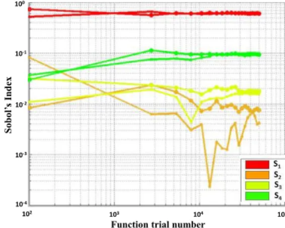
The first result obtained concerns the influence of the inputs of the model on the net charge density. An electric field of 30 kV/mm is applied during 100 s on a LDPE material and the charge profiles are computed and integrated over time and space. Sobol index calculations are computationally expensive and require a high number of calls to the studied function. To illustrate this, Fig. 2 shows a result for the convergence as a function trial number. Two trials are made at each step for each input. It can be seen that about 50 000 runs are necessary to reach convergence. This means 100 000 calls to functions for each parameter, and in total 500 000 calls for the all input parameters to guarantee the convergence of the Sobol's index. It represents about 30 hours to implement with a computer having an Intel Core i7-4790 processor, CPU of 3.60GHz and 32Go of RAM.
Fig. 2. Convervenge for the Sobol indexes calculation
Fig. 3 quantifies the amount of variance that each inputs xi
contributes to the total variance of the net charge density and current density. We note Si the Sobol index of the xi input and
Sij the index of order 2 between two inputs xi and xj. As shown
on this figure, the variance of a give contribution can be split in two parts: that caused by variations of individual inputs, which represent the main effect, and that caused by mutual interactions of several inputs. The sum of the total index reaches 1, which proves the independence of the different inputs and a good convergence of the algorithm (a value higher than 1 would mean redundancy between some input parameters). Concerning the Sobol's index for the net charge output, Fig. 3 shows that the barrier height of injection, x1,
plays an essential role in the first instants of the polarization: Sobol's index for the net charge density is affected by the charge injection at up to 60%. The de-trapping barrier and the interaction between injection / de-trapping represent only 10% each to the total variance of the y1 output. Other inputs are
negligible, meaning that, at the first moments of the polarization, mobility and trapping do not have substantial influence on the net charge density. This first result shows that injection phenomena could be analyzed nearly independently of the other physical phenomena. For parameters optimization,
100 10-1 10-2 10-3 10-4 102 103 104 105 So bo l’ s Index
the barrier height of injection could be estimated by fixing the others inputs at any value. Concerning the Sobol index for the current density output, the mutual interactions of inputs are more impacting that the individual inputs. The interaction injection / de-trapping represents 30% of the total variance while the individual input de-trapping concerns slightly less than 20% and injection phenomena about 10%. Note here that the total sum of indexes is less than 1, meaning that higher order interactions (involving 3 input parameters) are at play.
Fig. 3. Sobol indexes for the y1 and y2 output with charging time of 100 s
B. Impact of charging time
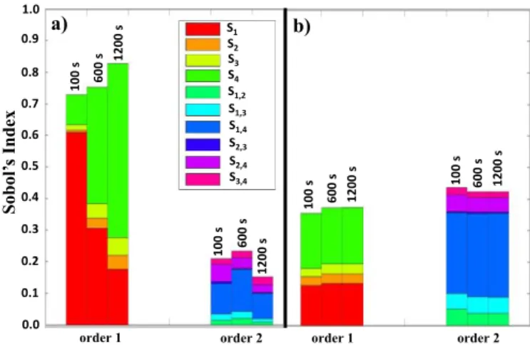
Fig. 4a) shows the evolution of Sobol indexes during polarization process for the y1 output (representing charge
density) with charging times of 100 s, 600 s and 1200 s. As explained previously, at the first moment of the polarization the injection process overwhelms the other parameters in terms of influence on the charge density. This trend tends to weaken over time. For 1200 s, de-trapping rises up to 55% while barrier height of injection drops to less than 20%. The other parameters, mobility and trapping do not have much influence on the output, at most 10% of the total variance. Finally, injection process, de-trapping and their interactions are impacting at up to 80%. Concerning indexes for the y2 output
i.e. current density, there is not much evolution over time, cf.
Fig 4b). Results show that interaction of order 2 is more impacting that the individual inputs. Here again, the sum of the total index does not reach 1.
By analyzing these results a strategy of study can be designed for parameters optimization. The first step would consist in fixing mobility and trapping coefficient to a random value and then optimizing de-trapping coefficient and barrier height of injection with the net charge density only, preferably using short time data. By constraining the variation interval of estimated parameters found in the first step, the optimization could then be realized with the current density as output and the others parameters, trapping and mobility, as inputs. Indeed, interactions between parameters being more important with the y2 output, the
optimization process could adjust more precisely each one. Beyond the current objectives, reverse uncertainty propagation can also be applied for identifying experimental favourable
conditions to reduce uncertainties on the parameters. For instance, local sensitivity indexes can be evaluated for experimental conditions (temperature, field, etc..) allowing detecting the configuration that is the less dependent on the most uncertain parameters. The measurements coming from these specific configurations could be used to calibrate the models.
Fig. 4. Evolution of Sobol indexes during polarization process with charging times of 100 s, 600 s and 1200 s a) for the y1 output and b) for the y2 output
V. CONCLUSION
A Sobol algorithm has been used in order to estimate the impact of parameters of a charge transport model on the observables for the charge build up in insulation that are charge density measurements and external current. The procedure has been tested on 4 variable parameters as model input, considering charge density and current predicted for up to 20 min charging time. We show that at short charging time (100s), the main influent model parameters for the charge distribution are barrier to injection and de-trapping coefficient. The exact reason for the impact of de-trapping is not really elucidated at present. For longer polarization time, the contribution from de-trapping rises and that from injection drops. Regarding charging current, the contributions to the Sobol index are mostly from mutual interactions between input parameters: this means that current analysis alone cannot easily unravel the different contributing processes to the macroscopic behaviour.
REFERENCES
[1] S. Le Roy, G. Teyssedre, G.C. Montanari, F. Palmieri, and C Laurent, “Description of charge transport in polyethylene using a fluid model with a constant mobility: fitting model and experiments”, J. Phys. D: Appl. Phys., vol. 39, pp. 1427-1436, 2006.
[2] J. M. Alison and R. M. Hill, “A model for bipolar charge transport, trapping and recombination in degassed crosslinked polyethylene”, J.
Phys. D: Appl. Phys., vol. 27, pp. 1291-1299, 1994.
[3] K. Kaneko, T. Mizutani and Y. Suzuoki, “Computer simulation on formation of space charge packets in XLPE films”, IEEE Trans.
Dielectr. Electr. Insul., vol. 6, pp. 152-158, 1999.
[4] S. Segonds, C. Gogu, Y. Qiu, C. Bes, A. Mauffrey. “Design optimization under evidence based uncertainty with application to an engine connecting rod”, International Journal of Design and Innovation Research, 5 (3), pp. 77-91, 2010.
[5] I.M. Sobol. “Global sensitivity indices for nonlinear mathematical models and their Monte Carlo estimates”, Mathematics and Computers in Simulation (55), pp. 271-280, 2001. 0.0 0.1 0.2 0.3 0.4 0.5 0.6 0.7 0.8 0.9 1.0
order 1, Si order 2 , Sij total index, Ssum of the
T Si for y1 Si for y2 Sforij y2 Sij for y1 SiT for y1 SiT for y2 So bo l’s Index S1, S1T S2, S2T S3, S3T S4, S4T S1,2 S1,3 S1,4 S2,3 S2,4 S3,4 10 0 s 6 0 0 s 1200 s a) 10 0 s 6 00 s 12 00 s 0.0 0.1 0.2 0.3 0.4 0.5 0.6 0.7 0.8 0.9 1.0 10 0 s 6 00 s 12 00 s 10 0 s 6 00 s 12 00 s
order 1 order 2 order 1 order 2
b) So bo l’ s Index S1 S2 S3 S4 S1,2 S1,3 S1,4 S2,3 S2,4 S3,4