HAL Id: hal-02271098
https://hal-mines-albi.archives-ouvertes.fr/hal-02271098
Submitted on 22 Nov 2019
HAL is a multi-disciplinary open access
archive for the deposit and dissemination of
sci-entific research documents, whether they are
pub-lished or not. The documents may come from
teaching and research institutions in France or
abroad, or from public or private research centers.
L’archive ouverte pluridisciplinaire HAL, est
destinée au dépôt et à la diffusion de documents
scientifiques de niveau recherche, publiés ou non,
émanant des établissements d’enseignement et de
recherche français ou étrangers, des laboratoires
publics ou privés.
Planning with preferences using Multi-Attribute Utility
Theory along with a Choquet Integral
Loïc Bidoux, Jean-Paul Pignon, Frederick Benaben
To cite this version:
Loïc Bidoux, Jean-Paul Pignon, Frederick Benaben. Planning with preferences using Multi-Attribute
Utility Theory along with a Choquet Integral. Engineering Applications of Artificial Intelligence,
Elsevier, 2019, 85, pp.808-817. �10.1016/j.engappai.2019.08.002�. �hal-02271098�
Planning with preferences using Multi-Attribute Utility Theory along with a
Choquet Integral
I
Loïc Bidoux
a,b, Jean-Paul Pignon
b, Frédérick Bénaben
a,< aIMT Mines Albi - University of Toulouse, FrancebThales Communications & Security, France
A R T I C L E I N F O
Keywords:Preference-based planning Multi-Attribute Utility Theory Choquet integral
ChoPlan
A B S T R A C T
This paper addresses the problem of planning with preferences using Multiple Criteria Decision Analysis (mcda) mechanisms. We start by explaining how pddl3 preferences can be modelled by criteria from the Multi-Attribute Utility Theory (maut) along with a Choquet integral. Interestingly, preferences formalized using maut have almost the same expressiveness as the ones formalized in pddl3 while being much easier to model. Next, we present a new heuristic for planning with preferences which is based on the Choquet integral. Finally, we introduce ChoPlan a proof-of-concept planner solving maut-encoded planning problems using the aforementioned heuristic. ChoPlan’s performances are evaluated with respect to state of the art planners using problems from the fifth International Planning Competition.
1. Introduction
Planning addresses the problem of finding a sequence of actions to achieve a specified goal state from a given initial state. In many real-world applications, the set of valid plans may be quite large as the aforementioned goal state may be achieved in various ways. As a consequence, it is crucial to consider the notion of plan quality to distinguish between good and bad plans according to users’ preferences. Preferences naturally arise in many use cases and can be illustrated using the Tourism domain (more details regarding this new planning domain in Section4) in which a road trip including visits of several cities and points of interest must be organized. In this problem, one may have preferences over the visits to perform or the restaurants and hotels to book based on criteria such as financial cost and comfort. Moreover, it may be preferred that some cities are visited before other ones. In order to compare plans based on their quality, a preference relation amongst the set of valid plans must be defined. The pddl3 (Gerevini and Long,2006) is the main language used by the planning community to construct such a relation. It has been extensively used during the fifth international planning competition (Gerevini et al.,2009) which focused on planning taking into account users’ preferences.
This paper studies the problem of planning with preferences using Multiple Criteria Decision Analysis (mcda) mechanisms. mcda assists users solving decision problems such as the identification of the best solutions amongst a large set of alternatives (seeFigueira et al.,2005 for a complete state of the art survey). Generating a preference model
I No author associated with this paper has disclosed any potential or pertinent conflicts which may be perceived to have impending conflict with this work. For full disclosure statements refer tohttps://doi.org/10.1016/j.engappai.2019.08.002.
< Corresponding author.
E-mail addresses: [email protected](L. Bidoux),[email protected](J.-P. Pignon),[email protected](F. Bénaben).
that formalizes decision-makers’ preferences is a key element of mcda. These models have a great expressiveness since they can represent several criteria as well as the various interactions between them. Con-sidering that mcda problems and planning with preferences presents some similarities, ideas from the mcda community can benefit the planning community. In this paper, we show that the mcda formalism brings practical improvement as it can be used to extend the scope of preference-based planning problems that can be solved. Furthermore, we introduce a new heuristic for planning with preferences inspired by some mcda mathematical tools.
In Sections2and3, we present preliminary notions on planning with preferences and mcda. In Sections4and5, we describe the contri-butions of this paper namely an extension of the pddl3 formalism as well as a new heuristic for preference-based planning. Next, in Section6, we introduce our planner ChoPlan and evaluate its performances with re-spect to state of the art planners. To conclude, applications to planning in crisis management context are briefly discussed in Section7.
2. Planning with preferences
In order to introduce the problem of planning with preferences, we first state the definition of the classical planning problem as described byGhallab et al.(2004).
Definition 1 (Classical Planning). A classical planning problem CP is a
actions, : S ù A ô S a transition function, s0À S an initial state, G a
goal formula and SG” S the set of goal states induced by G. A solution
of a problem CP is a sequence of actions x = Ía1, … , anÎcorresponding
to a sequence of states Ís1, … , snÎsuch that s1 = (s0, a1), … , sn =
(sn*1, an)and snÀ SG. The set of solutions (or plans) of CP is denoted
by X.
In many real-world applications, users may prefer some plans to others because they might have interesting properties, be easier or cheaper to implement. This motivates the introduction of a preference relation à over X such that x1 à x2 is interpreted as ‘‘plan x1 is at
least as preferred as plan x2’’. Preference-based planning (seeBaier and
McIlraith,2008for a complete survey) extends the classical planning approach by taking into account the relation à that represent users’ preferences.
Definition 2 (Preference-based Planning). A prefer-ence based planning
(PBP) problem is a pair I = (CP, Ã) with CP a classical planning
problem and à a complete preorder on X. A plan x is a solution of (CP, Ã) if x is a solution of CP. Moreover, x is an optimal solution if
≈x®À X, x à x®.
The goal of preference-based planning is to find optimal solutions (or at least good ones) according to à contrarily to classical planning where any solution is satisfactory. PBP problems are formalized us-ing the pddl3 language introduced in 2006. In pddl3, preferences are conditions on the sequence of states (also called trajectory) of a plan that users would prefer to see satisfied if possible. Preferences are defined using modal operators such as
at-end
,always
,sometime
,at-most-once
andsometime-before
whose semantics are de-scribed in Gerevini and Long (2006). Considered as soft constraints, preference formulas are always true from a semantic point of view but can nonetheless be satisfied or not. Penalties for violation are calculated using preference costs associated with Boolean expressions(is-violated <name>)
where<name>
is the preference’s name. Plan quality is specified by aggregating the various preference costs using the metric function introduced in pddl2.1 byFox and Long(2003).3. Preference modelling in MCDA
This section deals with preference modelling using the mcda for-malism. It focuses on the methods used in this paper namely the Multi-Attribute Utility Theory (maut) and the Choquet integral. Prefer-ence modelling aims to design a model that permits automatic analysis of how several alternatives (plans in our context) compare to each other. To this end, a complete preorder à (e.g. a reflexive and transitive binary relation) is defined over a set of alternatives X. Let P = {1, … , p} be the set of criteria to be considered in order to compare the alter-natives. Such criteria can be associated with any quantity such as a production cost, a delivery time or a level of quality for instance. Each alternative x À X is identified by an attribute tuple (x1, … , xp)of the
cartesian product ⌦ = ⌦1ù5ù⌦pwith ⌦k” R denoting the definition
domain of the criteria k.
3.1. Multi-attribute utility theory
The maut formalism (see Dyer, 2005) associates each alternative with a utility. This value represents the level of satisfaction of the decision-makers with respect to x and is expressed on a common
sat-isfaction scale ⇠ = [0, 1].
Definition 3 (MAUT Model). Given X a set of alternatives and P a set
of criteria, the maut model defines a complete pre-order à on X by: T
xa à xb € U(xa)g U(xb)
U(xi) = (u1(xi
1), … , up(xip))
with U : ⌦ ô ⇠ a maut utility function based on:
• uk: ⌦kô ⇠ some partial utility functions • : ⇠p ô ⇠ an aggregation function
Partial utility functions uk : ⌦k ô ⇠ have values within the
common satisfaction scale ⇠ = [0, 1]. A pure linear model (uk(xk) = kùxk, ≈xkÀ ⌦k) is not satisfactory to construct partial utility functions
as decision-makers preferences are generally not linear. Indeed, it is more suitable to consider continuous piecewise linear utility functions which provide a great expressiveness as they can approximate any continuous arithmetic function.
Definition 4 (Piecewise Linear Utility Function). Let uk be the partial
utility function of the criterion k À P . ⌦k is divided in n intervals,
bounds of which !0
k = 0, … , !nk = 1 are defined such that: ≈i À
[0, n * 1], !i
k < !i+1k . Utility of an alternative x À X on criterion k
is defined by linear interpolation of xkÀ [!ik, !i+1k ]with i À [0, n * 1]:
uk(xk) = uk(!ik) +
uk(!i+1k ) * uk(!ik)
!i+1 k * !ik
ù (xk* !ik)
Within the maut framework, the aggregation function is used to compute an alternative’s utility with respect to the values provided by the partial utility functions uk. Due to its simplicity, the weighted sum
is a commonly used aggregation function.
Definition 5 (Weighted Sum). Let y À ⇠p be a vector and w À [0, 1]pa
vector of weights such that≥p
k=1wk = 1with wk g 0. The weighted
sum Sw: ⇠pô ⇠ is defined as:
Sw(y) = p
…
k=1
wkyk
Unfortunately, the weighted sum has intrinsic limitations and thus cannot be used to model a possibly important spectrum of decision-makers preferences. In order to illustrate these limitations, let us con-sider the example proposed byGrabisch and Labreuche(2010). Three alternatives xa, xb, xc are to be compared, based on two criteria and
their respective utility functions u1 and u2so that:
u1(xa1) = 0.4 u1(xb1) = 0 u1(xc1) = 1
u2(xa2) = 0.4 u2(xb2) = 1 u2(xc2) = 0
If a decision-maker prefers to avoid solutions with totally unsatisfac-tory criteria (≈k À P , uk(x) ë 0), then its preferences induce the order
xa » xb Ì xc. As a consequence, the vector of weights (w1, w2)of S w
has to respect:
xbÌ xc € w
1= w2
xa» xb € 0.4 (w1+ w2) > w2
which is impossible. This type of behaviour is due to the implicit hypothesis of criteria independence inherent to the weighted sum. As a consequence, it is necessary to look for more powerful aggregation operators to model complex preferences. The Choquet integral is one of them.
3.2. Choquet integral
In order to design a model avoiding the aforementioned limitations, one can generalize the weighted sum by defining weights not only on single criterion but also on all possible subsets of criteria of P . Such a generalization is possible using the notion of capacity (Choquet,1953) which is defined over P(P ) the power set of P .
Definition 6 (Capacity). Let P be a set of criteria, the function : P(P ) ô [0, 1] is a capacity function if:
• (Á) = 0 and (P ) = 1
The capacity is normalized and increasing which is interpreted in the natural way. The notion of capacity allows us to introduce the Choquet integral (Choquet,1953) which can be used as an aggregation function.
Definition 7 (Choquet Integral). Let y À ⇠pbe a vector and a capacity
function defined over P(P ). The Choquet integral C : ⇠pô ⇠ is defined
as: C (y) = p … k=1 ({ (k), … , (p)}) ù [ y (k)* y(k*1)]
with a permutation on P such that y (1)f 5 f y (p)and y(0)= 0.
The Choquet integral generalizes the main usual aggregation oper-ators: min, max, weighted sum and ordered weighted sum (Grabisch, 1996). It permits us to model weighting as well as interactions between criteria. For instance, the notion of capacity provides a solution to the aforementioned example:
xbÌ xc € ({1}) = ({2})
xa» xb € 0.4 ({1, 2}) > ({2})
Choosing ({1}) = ({2}) = 0.3 allows us to design the expected preference model as ({1, 2}) = 1 by definition. Preference models based on a Choquet integral with respect to some capacity have a great expressiveness. However, their expressiveness comes at the price of complexity as 2p* 2parameters are required to define the capacity
function (i.e. all the values of on P(P ) except for Á and P ). In order to simplify these models while keeping most of their expressiveness,
Möbius transformation (Rota,1964) and k-additive capacities (Grabisch, 1997) are introduced.
Definition 8 (Möbius Transformation). Let be a capacity, its Möbius
transformation m : P(P ) ô [*1, 1] is given by:
m(A) = …
K”A
(*1)A‰K (K)
Definition 9 (K-additivity). A capacity is said k-additive if its Möbius
transformation verifies:
•≈A À P(P ), A > k Ÿ m(A) = 0 •«A À P(P ), A = k and m(A) ë 0
The k-additive capacities are particularly interesting because one only needs ≥k
i=1 pi parameters to represent them. In particular,
2-additive capacities are often considered as the best compromise be-tween expressiveness and complexity. They only required p (p + 1)_2 parameters to be specified while still allowing to model interactions between pairs of criteria (interactions between more than two criteria being hard to handle for decision-makers anyway). Using a 2-additive capacity, the Choquet integral can be expressed as followsGrabisch and Labreuche(2010).
Definition 10 (2-additive Choquet Integral). Let y À ⇠pbe a vector and
a capacity function defined on P . The 2-additive Choquet integral
C : ⇠pô ⇠ is defined as: C (y) = … Iij>0 (yi· yj) ù Iij+ … Iij<0 (yi‚ yj) ù Iij + … iÀPyi ù⌅ i* 12… iëj Iij ⇧
with · and ‚ denoting min and max operators, miand mijused instead of m({i}) and m({i, j}) for simplicity:
• Iij= mij
• i= mi+12≥iëjIi,j
The Shapley value i (Shapley,1953) expresses the global weight of the criterion i. It should not be confused with miwhich represents
the importance of the criterion i considered alone. Furthermore, the
interaction index Iij (Grabisch,1997) characterizes the interaction
be-tween criteria i and j. By analysingDefinition 10, one sees that if the interaction index Iij is positive, criteria are aggregated using the
min operator. In this case, the criteria are said complementary as their overall score is high only if both criteria scores are high. On the other hand, if the interaction index Iijis negative, the criteria are aggregated
using the max operator. In this case, they are said substitutable one to the other as it is sufficient that one criterion score is high in order to obtain a high overall score. Finally, the linear part of the integral performs the weighting of the individual criteria.
4. Modelling PDDL3 preferences using MAUT
In this section, we show that the pddl3 preferences can be expressed using the maut model and a Choquet integral. Interestingly, preferences formalized using maut have almost the same expressiveness as the ones formalized in pddl3 while being much easier to model. We first introduce a new planning domain (Section4.1) that will be used for illustrative purposes in the subsequent sections. Then, we explain how to encode pddl3 preferences into maut criteria and how to substitute the pddl metric function with a Choquet integral (Section4.2). Next, we present the formal language of our pddl3/maut extension (Section4.3). To finish, we compare the expressiveness of the pddl3/maut with respect to the initial pddl3 formalism (Section4.4) and explain why preference elicitation is easier to perform using pddl3/maut (Section4.5).
4.1. Tourism planning domain
We have introduced a new planning domain denoted Tourism in order to illustrate how the pddl3 preferences can be represented using a maut model along with a Choquet integral (Bidoux,2017c). In this domain, one has to organize a road trip between cities while optimizing several trajectory preferences (points of interest to visit before other ones or at most once, culinary specialities to try) and several numeric preferences (travel duration, financial cost, comfort, entertainment and cultural scores). Unsurprisingly, the travel duration criterion can be used to express a preference regarding the duration of the road trip. The financial cost criterion models the various expenses of the journey such as the travel costs or the hotels and restaurants prices. The comfort criterion models the quality of the considered hotels and restaurants. The entertainment and cultural criteria depends on the various points of interest that are visited. Some constraints ensuring that the road trip participants eat and sleep regularly must also be respected. In order to formalize the intrinsic interactions between these numeric preferences, the plan metric is modelled by a Choquet integral involving a substi-tutability between financial cost and comfort score as well as between entertainment and cultural scores.
4.2. Representing pddl3 preferences using maut
In the previous section, we have explained that a maut criterion is characterized by an attribute value (xk) along with a partial utility
func-tion (uk) representing the user’s preferences over the attribute domain
(⌦k). The pddl3 preferences can easily be generalized by substituting
each one of them with a maut criterion.
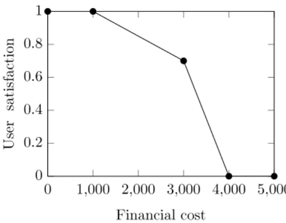
Such a substitution is quite intuitive for numeric preferences as one only needs to define the partial utility function of the considered numeric expression. For example, given a Tourism problem, a user may be completely satisfied (respectively totally unsatisfied) if the financial cost of the road trip is 1000 euros (respectively 4000 euros). Moreover, his preferences are not necessarily linear and he may strongly prefer a price of 3000 euros to one of 4000 euros while moderately preferring a price of 1000 euros over one of 3000 euros. These preferences are
Fig. 1. Example of an attribute’s partial utility function.
illustrated onFig. 1where the partial utility function is defined over
⇠ = [0, 1] with 1 and 0 denoting respectively complete satisfaction and
total dissatisfaction.
Encoding pddl3 trajectory preferences in maut criteria is less intuitive but nonetheless straightforward. Indeed, one only has to consider an at-tribute matching the semantic of the preference along with the identity as a partial utility function. For instance, in a Tourism problem,
pref-erence (sometime-before (c-visited
c2) (c-visited
c1))
means that the cityc1
should be visited before the cityc2
if possible. If a plan implies visitingc2
beforec1
, then the preference is violated, the value of the corresponding maut attribute and its partial utility are both equal to 0. On the other hand, ifc1
is visited beforec2
(or if
c2
is never visited), then the preference is satisfied by the plan, the value of the maut attribute and its partial utility are both equal to 1. This simple mechanism allows pddl3 preferences to be represented by maut criteria while preserving their initial semantic.As in pddl3, plan quality (called utility in the maut terminology) is obtained by merging the problem’s criteria using an aggregation operator.
Preference aggregation is more intuitive in the maut model as it enforces commensurability between criteria. Indeed, all preferences are defined using a partial utility function over the same satisfaction scale
⇠. We illustrate this using the Tourism problem once again. Hotels that
may be booked during the road trip are characterized by a comfort score defined with respect to the following values:
high, moderate
and
low
. Without commensurability, it is impossible to determine if an improvement on the financial cost preference (e.g. a cost of 1800 euros rather than 2200 euros) is preferred to one on the average comfort score preference (e.g. from amoderate
comfort score to ahigh
one). Therefore, constructing a metric function aggregating meaningfully financial cost, comfort score andsometime-before (c-visited
c2) (c-visited c1)
is difficult in pddl3. On the contrary, if pref-erences are represented by maut criteria, it is easier to aggregate them as they are all commensurable.Preference aggregation is performed using the Choquet integral along with a 2-additive capacity. As explained in Section3, a 2-additive capacity can be used to represent the weight of each preference as well as the interactions between pairs of preferences. For illustrative purpose, we present in Fig. 1 a capacity aggregating financial cost (criterion 1), average hotel comfort score (criterion 2) and
sometime-before ((c- visited c2) (c-visited c1))
(criterion 3) pref-erences. If the user considers that criteria 1 and 2 are equally important and slightly more important than criterion 3, its preferences can be represented by ({1}) = ({2}) > ({3}). Moreover, if he estimates that there is no interaction between pairs of criteria (1, 3) and (2, 3), we have ({1}) + ({3}) = ({1, 3}) and ({2}) + ({3}) = ({2, 3}). Finally, the user may think that 1 and 2 are substitutable ( ({1}) + ({2}) > ({1, 2})) which means that he may accept a high financialTable 1
Example of a 2-additive capacity.
P(P ) Á 1 2 3 12 13 23 123
0 0.5 0.5 0.4 0.6 0.9 0.9 1
m 0 0.5 0.5 0.4 *0.4 0 0 0
cost if the average hotel comfort score is also high and vice versa. Table 1illustrates a 2-additive capacity satisfying these requirements. When instantiated with such a capacity, the Choquet integral defines an aggregation function for the three aforementioned criteria and their interactions.
4.3. Formal language of the pddl3/maut extension
As the intuition regarding the generalization of the pddl3 prefer-ences into maut criteria have been explained, we now present the formal language of the pddl3/maut extension. We have chosen to de-sign this extension such that it is fully compatible with the existing pddl3 specification. In order to do so, we have introduced a new pddl requirement that planners may choose to support. The latter is called
maut-preferences
and is built uponnumeric-fluents
and
preferences
requirements (Gerevini and Long,2005). The bnf description specifying the syntax of themaut-preferences
require-ment is available on dataverse (Bidoux,2017a). Without any surprise, the main elements of this extension are the concepts of maut cri-terion (<maut-criterion>
) and the concept of Choquet integral (<choquet-integral>
).In addition, in order to define the semantics of the pddl3/maut ex-tension, one only need to combine the semantics of the pddl2.1 numeric expressions (Fox and Long,2003) and the pddl3 preferences (Gerevini and Long,2006) with respect to the maut definitions. We now precise the definitions given in Section2in order to formalize the semantics of the pddl3/maut extension.
Definition 11 (PDDL3 Planning Problem). An instance of a pddl3
plan-ning problem is defined to be a pair I = (Dom, P rob) where:
• The planning domain is a tuple Dom = (F, R, A) consisting of function symbols F , relation symbols R and actions A.
• The planning problem is a tuple P rob = (O, s0, EG, P ) consisting of objects in the domain O, initial state s0, extended goals EG and
preferences P .
Definition 12 (PDDL3/MAUT Planning Problem). An instance of a
pddl3/maut planning problem IM is an instance of pddl3 planning
prob-lem I where the tuple P rob have been redefined as (O, s0, EG, MC, C )
with MC a set of criteria representing the preferences P of the problem and C a 2-additive Choquet integral.
In such problems, a state s is no longer defined as a set of atomic formulas Atm but as a pair (Atm, v) with v À Rdimwhere dim denotes the
number of primitive numeric expressions of the problem (Fox and Long, 2003). Based on these additional notations, we can define the utility associated to both numeric and trajectory preferences and explain how the plan’s utility is computed.
Definition 13 (Numeric Preference Utility). Let t = Ís0, … , snÎ be a
trajectory whose final state sn is described by the pair (Atm, v), f be
a primitive numeric expression and k À MC be the maut criterion representing the numeric preference with attribute f and partial utility function uk: ⌦fô[0, 1]. The utility associated to the maut criterion k
on the trajectory t is computed with respect to snas utk= uk(vf).
Definition 14 (Trajectory Preference Utility). Let t = Ís0, … , snÎbe a
trajectory, be an extended goal and k À MC be the maut criterion representing the trajectory preference associated to with partial
utility function uk: {0, 1} ô [0, 1]. The utility associated to the maut criterion k on the trajectory t is computed with respect to the semantic of as: ut k= T 1 if Ís0, … , snÎ Ù 0 if Ís0, … , snÎ Ù ¬
Definition 15 (Plan Utility). Let IM be an instance of a pddl3/maut problem, x be a plan defined by the trajectory t and ut
1, … , utpthe partial
utility values of the maut criteria MC with respect to t. The utility U of the plan x is defined as Ux= C (ut1, … , utp).
UsingDefinition 15, a plan x1is said at least as preferred as a plan
x2(denoted x1Ã x2) if and only if Ux1g Ux2.
4.4. Comparison between pddl3 and pddl3/maut
We have chosen to design the pddl3/maut extension so that it is fully compatible with the existing pddl3 specification. Therefore, it comes at no surprise that pddl3 and pddl3/maut are almost identical in term of expressiveness. One should nonetheless note that some differences exist between these two formalisms.
In order to represent a numeric preference within the pddl3/maut formalism, one has to bound its value which is not required in pddl3. From a strict theoretical viewpoint, this means that some pddl3 prob-lems cannot be encoded into pddl3/maut unless bounds on numeric val-ues are provided in order to convert them. However, working with un-bound numeric preferences induce incommensurability between prefer-ences which in turn impacts negatively the preference aggregation. As such, one can argue that when working on real world problems where the preference model have to be meaningful, one should have avoided unbounded numeric preferences in the beginning.
On the other hand, the pddl3/maut formalism brings several im-provements in term of expressiveness with respect to the pddl3. By the very nature of maut criteria, it is possible to aggregate several criteria together in order to produce a new one. Consequently, the notion of compound preferences aggregating several preferences can be used in pddl3/maut while not being supported in pddl3. One should note that compound preferences are also supported by others PBP languages such as LPP for exampleBienvenu et al.(2006).
In addition, in pddl3 preferences are intrinsically binary whereas they are intrinsically fuzzy in pddl3/maut thanks to the employed partial utility functions. Therefore, pddl3/maut preferences could be used to generalize pddl3 preferences thus increasing the expressiveness of the language. For instance, a pddl3/maut preference could be used to count the number of states in which a predicate is true thus constituting a fuzzy interpretation of the pddl3
(sometime
) preference that only express whether is true at least once in the plan.4.5. Preference elicitation using pddl3/maut
Preference elicitation is the process used to create a mathematical representation of user’s preferences with respect to a relation Ã. As the automated planning community is mainly focused on problem solving, the preference elicitation problem (which constitutes one step of the problem modelling) is generally assumed solved a priori by current preference-based planning approaches. One might consider this posture slightly dogmatic as in many real-world PBP applications, preference elicitation is a crucial problem to address and can be as hard to solve as the planning problem itself. Indeed, there is no point to look for an optimized solution with respect to a given preference model if the latter does not formalize correctly what the decision-makers are trying to achieve.
Preference elicitation is intrinsically easier to perform using the pddl3/maut formalism. Indeed, the latter natively supports (i) fine-grained definition of preferences thanks to partial utility functions, (ii) commensurability between preferences (which enforces meaningful
preference comparison) thanks to the common satisfaction scale ⇠ as well as (iii) preference interactions thanks to the Choquet integral. Even if such mechanisms could be simulated in pddl3, doing so would com-plexify a lot the underlying planning problems as these functionalities cannot be easily formalized in plain pddl3. This is illustrated by the
Tourism planning domain that features several trajectory preferences
(points of interest to visit before other ones or at most once, culinary specialities to try), several numeric preferences (financial cost, travel duration, comfort, entertainment and cultural scores) as well as several constraints to respect. In addition, its plan metric is modelled by a Choquet integral involving substitutability between criteria. One should note that the Tourism domain contrasts with many IPC5 planning domains that use at most one numeric preference.
One should also note that several mcda results can be used to assist users during the creation of their preference models. For instance, when preferences are represented by maut criteria aggregated with a Choquet integral, the preference elicitation problem can be solved using a method proposed byLabreuche and Grabisch (2003). The latter is based on a questioning procedure in which the decision-maker is asked a few questions regarding its preferences over hypothetical alternatives maximizing subsets of criteria. This approach is quite interesting be-cause (i) the decision-maker is not required to have any mathematical background and (ii) no concrete plans have to be provided. Further-more, this preference elicitation method can be performed efficiently using the myriad software (Labreuche and Lehuédé,2005).
5. PBP using the Choquet integral
In Section4, the Choquet integral has been considered as a tool for preference modelling. Hereafter, it is used to define a new family of heuristics for planning with preferences (Section5.1). In addition, we present a new estimate of plan quality using fuzzy preferences (Section 5.2). Moreover, we also describe an algorithm solving PBP problems thanks to the aforementioned heuristics (Section5.3).
5.1. Heuristics based on the Choquet integral
Heuristic search has been a time-honoured principle to solve clas-sical planning problems in which several goals must be achieved. However, when planning with preferences, finding a solution is not enough as we are looking for good solutions according to user’s pref-erences. If the search is focused on goals, it might be easier to find solutions but these are likely to be mediocre ones with respect to preferences. At the opposite, if the search is only focused on prefer-ences, it is possible that no solution may be found at all. Our approach utilizes a heuristic search that performs a trade-off between easiness of achieving the goals and potential quality according to preferences. To this end, we rely on a 2-additive Choquet integral with respect to a capacity ⇢ along with two maut criteria respectively related to goals to
be achieved (denoted ) and preferences to be optimized (denoted ⇤). The
core idea is to define ⇢ to represent a complementarity (i.e. a positive interaction) between goal and preference criteria. As a consequence, all other things being equal, balanced solutions that are good on both goal and preference criteria will obtained a better score than imbalanced ones.
Definition 16 (Choquet-based Heuristic). Let I be a PBP problem
in-stance, C⇢be a Choquet integral and s a state, a Choquet-based heuristic
hcis defined as:
hc(I, s) = C⇢ (I, s) , ⇤(I, s)
where (I, s) and ⇤(I, s) are estimates related to goals to be achieved and preferences to be optimized respectively.
We now introduce h1
c a Choquet-based heuristic compatible with
the pddl3/maut formalism that is based on two criteria 1and ⇤1. The
goal criterion 1represents the progress made in order to achieve the
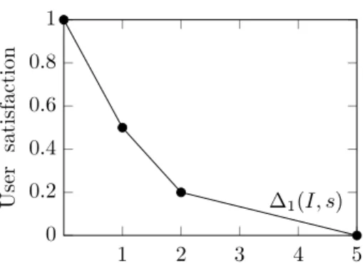
Fig. 2. Partial utility function uc.
value is computed using a relaxed planning graph along with the fast-forward heuristic ff (Hoffman and Nebel,2001). The latter estimates the minimal number of actions that one has to execute from s in order to achieve the goals G of the problem I.
Definition 17 (Estimate 1(IM, s)). Let IMbe an instance of a pddl3/
maut problem with G the goals to be achieved, s be a state and ucthe
partial utility function depicted onFig. 2, then:
1(IM, s) = uc⇠ ff(Iff(IM, s, G) M, s0, G)
⇡
Fig. 2illustrates the partial utility function uc. The user is
moder-ately satisfied (uc(1) = 0.5) if the state s is at the same distance of the
goals than s0. His satisfaction is maximal when the goal is verified in s
(uc(0) = 1). Moreover, his satisfaction slowly decreases between 1 and 2 in order to allow the planner to search for long solutions (whose quality might be better) even if the goals can be achieved quickly.
The preference criterion (denoted ⇤1) represents an estimate of the
quality of any plan that would be constructed by extending the state
s. It can be computed easily by evaluating the utility function of the
problem IMwith respect to the trajectory Ís0, … , sÎ. This estimate is
in-herently optimistic (respectively pessimistic) regarding the preferences satisfied (respectively violated) in Ís0, … , sÎ.
Definition 18 (Estimate ⇤1(IM, s)). Let IM be an instance of a pddl3/
maut problem with C its Choquet integral and ut
1, … , utp the partial
utility values of the p criteria of IM with respect to the trajectory
t = Ís0, … , sÎ,
⇤1(IM, s) = C (ut1, … , utp)
Following the definition of 1 and ⇤1, we now describe the h1c
heuristic.
Definition 19 (Heuristic h1
c). Let IM be a pddl3/maut problem and C⇢
be a Choquet integral,
h1c(IM, s) = C⇢ 1(IM, s) , ⇤1(IM, s)
5.2. Estimate of plan quality using fuzzy preferences
In this section, we describe an estimate of plan quality denoted ⇤2
that will be used to construct a second Choquet-based heuristic h2 c. This
estimate is presented using the pddl3/maut formalism but is nonetheless generic and could be built with any language supporting the notion of fuzzy preferences.
Using the preference criterion ⇤1, one implicitly considers that the
utility of an intermediate state of a plan is a good estimate of its final utility. Indeed, estimate ⇤1 takes into account the relative importance
of the preferences but does not consider any information regarding the future evolution of their satisfiability. One can design a more informed estimate by considering the likelihood that the preferences will be
satisfied in the final state given the current state s. For instance, one of the heuristics proposed byBaier et al.(2009) evaluates the metric function of the problem in various nodes Niof a relaxed planning graph
and then weights these values according to the depth i of the nodes Ni.
Moreover, the heuristic used in lprpg-p (Coles and Coles,2011) can be interpreted as a modification of the relaxed planning graph structure in order to take into account the preferences of the problem and their respective weights. The approach adopted in this work also exploits the relaxed planning graph structure yet is based on the fuzzy nature of the maut criteria used to represent the preferences.
The quantity ⇤2 is constructed by replacing in ⇤1 the usual
se-mantic interpretation of final preferences,
sometime
andsometime-before
preferences by an estimate of the effort to produce in order to satisfy them from the state s. One should note that this interpretation is compatible with the pddl preferences’ semantics since the two boundary cases of a null effort or an infinite effort can be seen respectively as a preference satisfied or violated in s. In order to redefine the semantics of the maut criteria, one can use mechanisms similar to those ofDefinition 17. For instance, ff(I, s, ) is an estimate of the number of actions that one has to execute from a state s to achieve the predicate . Thus, it describes the effort to produce in order to satisfy the pref-erenceat-end
from s. We now introduce formally the semantically redefined partial utility values associated to final preferences as well assometime
andsometime-before
preferences.Definition 20 (Utility of Final Preferences in ⇤2). Let IMbe a pddl3/maut
problem, t = Ís0, … , sÎ a trajectory, the formula associated to the final
preference represented by the maut criterion k À MC and ucthe partial
utility function depicted inFig. 2. The semantically redefined utility associated to the maut criterion k on the trajectory t is computed as:
Ñut k = h n n l n n j uc⇠ FF(IFF(IM, s, ) M, s0, ) ⇡ if FF(IM, s0, ) ë 0
1 if FF(IM, s0, ) = 0 and FF(IM, s, ) = 0
0 if FF(IM, s0, ) = 0 and FF(IM, s, ) ë 0
Definition 21 (Utility of
Sometime
Preferences in ⇤2). Let IM be apddl3/maut problem, t = Ís0, … , sÎ a trajectory, the formula associated
to the
sometime
preference represented by the maut criterion k À MC and ucthe partial utility function depicted inFig. 2. The semantically redefined utility associated to the maut criterion k on the trajectory t is computed as: Ñut k = h n n l n n j uc⇠ FF(IFF(IM, s, ) M, s0, ) ⇡ if FF(IM, s0, ) ë 01 if FF(IM, s0, ) = 0 and FF(IM, s, ) = 0
0 if FF(IM, s0, ) = 0 and FF(IM, s, ) ë 0
Definition 22 (Utility of
Sometime-before
Preferences in ⇤2). LetIMbe a pddl3/maut problem, t = Ís0, … , sÎ a trajectory, p a
sometime-before
( ) preference represented by the maut criterion k À MCand ucthe partial utility function depicted inFig. 2. The semantically
redefined utility associated to the criterion k on the trajectory t is computed as: Ñut k = h n n n n n l n n n n n j uc⇠ FF(IFF(IM, s, ) M, s0, ) ⇡ if t Ù p and FF(IM, s0, ) ë 0 1 if t Ù p and FF(IM, s0, ) = 0 and FF(IM, s, ) = 0 0 if t Ù p and FF(IM, s0, ) = 0 and FF(IM, s, ) ë 0 0 if t Ù ¬ p
As
always
andat-most-once
preferences do not have a natural fuzzy interpretation, we define their utility in ⇤2 as Ñutk= utkwhere utkis defined according toDefinition 14. Thanks toDefinitions 20to22, we can now describe the ⇤2estimate as well as the h2cheuristic. Definition 23 (Estimate ⇤2(IM, s)). Let IM be an instance of a pddl3/
maut problem, C its Choquet integral and Ñut
1, … , Ñutp the semantically
redefined partial utility values of the p criteria of IM regarding the
trajectory t = Ís0, … , sÎ, then:
⇤2(IM, s) = C (Ñut1, … , Ñutp)
Definition 24 (Heuristic h2
c). Let IM be a pddl3/maut problem and C⇢
be a Choquet integral,
h2c(IM, s) = C⇢ 1(IM, s) , ⇤2(IM, s)
The Choquet integral C⇢ which is used to aggregate the goal and
preference criteria of h1
c and h2c should not be confused with the
Choquet integral C which is used to aggregate the various preferences of the problem. In order to fully describe a Choquet-based heuristic, the capacity ⇢ must be specified. It turns out that defining ⇢ in a domain-independent way is not trivial. This problem is addressed in the next session.
5.3. Algorithm using Choquet-based heuristics
Algorithm 1 has been designed to solve PBP problems. The lat-ter uses standard planning techniques namely a forward search in a graph (
selectionRule
) using a best first approach (BFS) based on the aforementioned Choquet heuristics. In addition, it relies on two standard pruning rules (prunningRules
) that respectively sort out actions whose prerequisites are not satisfied in the current state s and actions whose execution would lead to a state s®in which one of thetrajectory constraints (also known as extended goals) of the problem would be violated.
In a nutshell, the algorithm works as follows: first, the neigh-bourhood of the initial state s0 is constructed (
selectionRule.
initFrontier(
s0)
) by considering all the states s that can beob-tained by executing an action a of the problem in s0(
IsApplicable
(current, action)
). During this step, the various pruning rules are triggered (IsPrunable(prunningRules, current, action)
) in order to not include in the neighbourhood of s0 states thatcan-not be reached from s0 as well as the states violating one of the
trajectory constraints of the problem. Next, the various states consti-tuting the neighbourhood of s0 are added to the list of nodes to be
considered (
Expland(current, action)
andselectionRule.
updateFrontier(child)
). This list is sorted according to the cho-sen Choquet-based heuristic (h1c or h2c) and the state s with the best
score is picked (
selectionRule.selectNode()
). The algorithm continues by adding the neighbourhood of s to the aforementioned list. This process is repeated until a state satisfying all the goals of the prob-lem (current.evaluate(
G)
) is found. Finally, the utility (i.e. the plan metric) of the solution is computed (current.getUtility()
). Algorithm 1 is iterative and as such does not terminate when a solution is found (solution.add(current)
) but instead continues to look for better solutions, thus incrementally producing plans of increased quality. This mechanism constitutes one of the key features of the algorithm as it is used in order to avoid the formalization of the heuristics’ capacity ⇢. Indeed, the algorithm will restart from the be-ginning (selectionRule.nextIteration(
s0)
) using a differentcapacity ⇢ each time a new solution is found. The capacity is chosen
so that each solution is generally harder to find than the previous ones but is likely to have a better quality according to preferences. Using Möbius representation, this can be done starting from capacity m0
⇢(see
Table 2) by decreasing the weight of by ↵ and increasing the weight of _⇤ by ↵ each time a solution is found until we get the capacity mf
⇢
that models a perfect complementarity between goal and preference criteria. Using this strategy, the Choquet-based heuristic is guided only by goals at first but these become less and less important in favour of preferences each time a new solution is found. This approach fully exploits the expressiveness of the Choquet integral. Indeed, the capacity
⇢ is constructed by considering a positive interaction I_⇤ between
goal and preference criteria thus modelling a complementarity between them. The higher ↵ is, the more difficult the problem becomes to solve between two iterations. It is therefore advisable to pick a small ↵ while ensuring that the quality improvement between two consecutive solutions does not become negligible. Performed experimental tests suggest that the empirical value ↵ = 0.1 is a good choice. Besides, varying the value of ↵ over the interval [0.05, 0.15] have only a marginal impact on the algorithm’s performances.
Algorithm 1: Choquet-based PBP algorithm Input: s0initial state of the problem
G goal formula of the problem A set of actions of the problem
Output: solution list of solutions to the problem Data: selectionRuleheuristic-based BFS
prunningRulesset of pruning rules currentcurrent node used in the search childnode expanding current
Algorithm
Search(
s0, G, A, Ã)
selectionRule.
initFrontier(
s0)
whileResourcesNotExhausted
andselectionRule.
isFrontierEmpty()
= Falsedocurrent } selectionRule.
selectNode()
if current.
evaluate(
G)
= Truethen if current.getUtility()
>solution.
getBestUtility()
thensolution.
add(
current)
end
selectionRule.
nextIteration(
s0)
elsefor all action À A do
if
IsApplicable(
current, action)
and
IsPrunable(
prunningRules,current, action
)
= Falsethenchild }
Expand(
current, action)
selectionRule .
updateFrontier(
child)
end end end end return solutionTable 2
Evolution of m⇢through iterations.
_⇤ ⇤ m0 ⇢ 1 0 0 mi ⇢ 1 * ↵ ù i ↵ ù i 0 mf⇢ 0 1 0
6. Implementation and evaluation
The proof-of-concept planner ChoPlan implements the algorithm and heuristics presented in Section5. It relies on the pddl4j library ( Pel-lier,2015), solves maut-encoded PBP problems and supports all pddl3 operators except those relying on time (
within
for instance).In order to evaluate ChoPlan’s performances, we have considered problems from International Planning Competitions (IPC) involving the whole set of pddl3 operators. Problems from the qualitative preferences track of IPC5 (Gerevini et al.,2009) are the only ones satisfying these conditions. We have restricted ourselves to the Rovers and Openstacks domains as the three other candidates (Storage, TPP and Trucks) are defined using
forall
andexists
pddl keywords that are not yet supported by ChoPlan. These domains are associated with 20 problems (denoted as SP) using final preferences only as well as 20 problems (denoted as QP) using any trajectory preferences. We have also cre-ated 20 problems (denoted as MP) using several numeric preferences and involving interactions between preferences for both considered domains. In addition, we have designed 20 MP problems for the Tourism domain introduced in Section 4.1. These problems aim to illustrate that preference modelling is easier to perform using the pddl3/maut extension .ChoPlan has been compared to all planners that have attempted
Rovers and Openstacks domains during IPC5 namely SGPlan 5.1 (Hsu et al., 2006), HPlan-P (Baier et al., 2009) and mips-xxl (Edelkamp and Helmert, 2001). As SGPlan 5.1 performs some domain specific optimizations, we have also included a variant SGPlan-w that disables the aforementioned optimizations following the procedure described byColes and Coles(2011). We have also considered the lprpg-p plan-ner (Coles and Coles, 2011) as well as three configurations of our planner. The ChoPlan 1 and ChoPlan 2 configurations are respectively instantiated with heuristics h1
c and h2c. The Control configuration is a
non-iterative version of the algorithm presented in Section5.3 instan-tiated with heuristic h1. Consequently, executing the Control planner
is equivalent to performing a best-first search with the fast-forward heuristic.
All the tests have been executed on the same machine, the latter using a 3.4 GHz i5-3570K CPU. Planners have been allowed to use at most 10 min of CPU-time to solve each problem and only the best solu-tion found for each problem have been considered. Furthermore, plan metric was computed using the plan validator val (Howey et al.,2004). Val permits to compare ChoPlan to other planners in a meaningful way even if the latter solves maut-encoded versions of the pddl problems.
Tables 3and4respectively shows the number of solutions found by each planner and the IPC score obtained by each planner (IPC score computation is explained in Table 4 caption). We stress that these results only constitute a preliminary evaluation of ChoPlan as they exclusively include planning domains supported by the current implementation of ChoPlan. In particular, one should note that this evaluation is intrinsically biased against lprpg-p. Indeed, the latter cannot solve the Openstacks problems but can solve some problems that have not been considered here (see Coles and Coles,2011for a precise evaluation of lprpg-p). Overall, SGPlan 5.1 is the best performing planner. Nevertheless, its performances seems to heavily rely on the domain-specific optimizations it employs as SGPlan-w is globally out-performed by all other planners. Of the remaining planners, ChoPlan obtains the best IPC scores on both SP and QP problems for the considered domains. However, given the number of solutions it found
Table 3
Number of problem solved. Symbol ‘‘–’’ denotes problems that cannot be solved due to unsupported pddl requirements. # Soluti ons Contr ol SGP lan 5.1 SGP lan -w HPlan-P mip s-xxl lprpg-p ChoPla n 1 ChoPla n 2 Rovers SP 20 20 20 – 20 20 20 20 Openstacks SP 18 20 0 20 20 – 18 18 Total SP 38 40 20 20 40 20 38 38 Rovers QP 16 20 4 14a 16 19 16 16 Openstacks QP 18 20 0 18a 20 – 18 18 Total QP 34 40 4 32a 36 19 34 34 Total 72 80 24 52 76 39 72 72 Rovers MP 20 – – – – – 20 20 Openstacks MP 20 – – – – – 20 20 Tourism MP 20 – – – – – 20 20 Total MP 60 – – – – – 60 60
aIndicates results from IPC5 competition (for planners that we have not succeeded to operate properly).
Table 4
IPC quality score. Symbol ‘‘–’’ denotes problems that cannot be solved due to unsupported pddl requirements. Let ⇧ be a set of planners and P be a set of problems, the score of a planner ⇡ on a problem p is defined as score(⇡, ⇧, p) = best * quality(⇧, p) ÷ quality(⇡, p). IPC score of a planner ⇡ on P is defined as IP C(⇡, ⇧, P ) =≥pÀP score(⇡, ⇧, p). IPC scor e Contr ol SGP lan 5.1 SGP lan -w HPlan-P mip s-xxl lprpg-p ChoPla n 1 ChoPla n 2 Rovers SP 15.30 19.06 15.41 – 15.73 13.09 15.73 15.60 Openstacks SP 1.85 15.82 0 10.03 2.32 – 3.74 9.97 Total SP 17.15 34.88 15.41 10.03 18.05 13.09 19.47 25.57 Rovers QP 8.90 18.02 1.53 9.76a 8.43 11.49 13.30 13.53 Openstacks QP 5.41 19.92 0 15.29a 6.21 – 15.93 11.71 Total QP 14.31 37.94 1.53 25.05 14.64 11.49 29.23 25.24 Total 31.46 72.82 16.94 35.08 32.69 24.58 48.70 50,81 Rovers MP 15.89 – – – – – 18.68 19.49 Openstacks MP 3.23 – – – – – 8.31 20 Tourism MP 14.48 – – – – – 18.50 17.14 Total MP 33.60 – – – – – 45.49 56.63
aIndicates results from IPC5 competition (for planners that we have not succeeded to operate properly).
on various problems, ChoPlan might scale less efficiently than some other planners. Regarding MP problems, both ChoPlan 1 and ChoPlan 2 bring significant improvements with respect to the Control planner.
IPC scores of ChoPlan 1 and ChoPlan 2 respectively corresponds to performance improvements of 45% and 65% with respect to the Control planner. Therefore, the h2
c heuristic brings a greater improvement of
plans’ quality than heuristic h1
c. This result is not surprising as the ⇤2
estimate can be seen as a more informed variant of the ⇤1 estimate
(see Section5.2). Nevertheless, despite better overall performances, ChoPlan 2 does not always outperform ChoPlan 1. On the contrary, the latter obtains superior results in three out of seven types of considered problems.
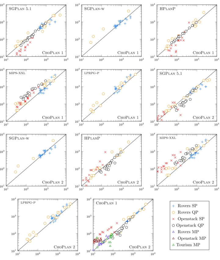
As appreciating planners’ relative performances using only the IPC score may be complex (especially when some planners do not solve the same problems than others), a comparison based on mutually solved problems is provided in Fig. 3. It shows that regarding the two considered domains, ChoPlan 1 is outperformed by SGPlan 5.1 and HPlan-P but outperforms SGPlan-w, mips-xxl and lprpg-p. Similarly, ChoPlan 2 is outperformed by SGPlan 5.1, behaves similarly as HPlan-P and outperforms SGPlan-w, mips-xxl and lprpg-p. Ultimately, results from Tables 3and4as well asFig. 3suggest that Choquet-based heuristics are interesting candidates in order to solve PBP problems.
Fig. 3. Comparison of planners on mutually solved problems (based on metric function value).
7. Applications
In this section, we briefly discuss the use of automated planning in crisis management contexts. This domain constitutes a natural ap-plication for this work as it can greatly benefit from our mcda-based planning with preferences approach. One can define a crisis as ‘‘a situation with long-term consequences due to an event that has caused extensive damage and losses resulting in an interruption of one or more critical activities within some part of the world’’ (CCA, 2014). Such situations may, for instance, result from natural disasters (tsunamis,
earthquakes, floods. . . ) or from industrial accidents. Planning problems for crisis management are rather different from traditional automated planning problems. They tend to be easier to solve as they are usually less combinatorial while being much harder to model. Indeed, it is quite difficult to represent the goals to achieve as determining the best strategy to handle the situation efficiently is generally crisis-specific and might be subject to debate amongst decision-makers. Planning in crisis management contexts requires to use a user-centric approach in order to convince the decision-makers that the proposed solutions are of interest.
An example of crisis management planning illustrating the use of our mcda-based approach is provided inBidoux et al.(2017b). In the considered scenario, decision-makers have to handle the crisis that is going to be caused by a massive flood event in Northern Europe using the capabilities of various first responder teams. To this end, decision-makers realize several preference models using the following criteria and their respective interactions: (i) the effectiveness of rescue operations, (ii) the comfort of the inhabitants of an area exposed to an isolation risk (which depends on whether food is supplied to them), (iii) the financial cost of the response, (iv) the necessity to resort on international aid proposed by neighbouring countries and (v) the capability to provide electricity to a critical company during some part of the crisis response. We defer the interested reader toBidoux et al. (2017b) andBidoux(2016) for additional details on the solution plans found by ChoPlan with respect to each preference model considered by the decision makers.
8. Conclusion
In this paper, we have explored the problem of planning with pref-erences expressed within the maut formalism along with a 2-additive Choquet integral. It turns out that planning can benefit from this mcda formalism on both practical and theoretical viewpoints. On the practi-cal side, we have shown that the pddl3/maut extension has almost the same expressiveness as the pddl3 language while facilitating preference modelling. On the theoretical side, we have introduced two Choquet-based heuristics as well as a new algorithm for PBP. This algorithm has been implemented in the ChoPlan planner whose performances have been compared to state of the art planners. Experimental results suggest that ChoPlan is an efficient planner for solving problems in which trade-offs between many goals and preferences have to be made. In addition, ChoPlan can be employed to address real operational planning problems as it has been incorporated in an information system for planning in crisis management contexts. Future work may include the improvement of ChoPlan to support all quantifiers, the improvement of the pddl3/maut extension to support time-based operators as well as the creation of new Choquet-based heuristics based on more advanced estimates.
Acknowledgments
Authors would like to thank Jorge Baier and Sheila McIlraith for their assistance regarding the use of HPlan-P. This work has been partially funded by ANRT under the grant 2012/1334.
References
Baier, J.A., Bacchus, F., McIlraith, S.A., 2009. A heuristic search approach to planning with temporally extended preferences. Artificial Intelligence 173 (5), 593–618. Baier, J.A., McIlraith, S.A., 2008. Planning with preferences. AI Mag. 29 (4), 25–37.
Bidoux, L., 2016. Planification avec préférences basée sur la Théorie de l’Utilité Multi-Attribut couplée à une intégrale de Choquet: application à l’interopérabilité des organisations en gestion de crise. (Ph.D. thesis). Mines-Albi, University of Toulouse.
Bidoux, L.c., 2017a. BNF description of the PDDL3/MAUT extension, DOI:http://dx.doi. org/10.7910/DVN/QDKBCF, Harvard Dataverse, v1.
Bidoux, L.c., 2017c. PDDL3/MAUT Tourism domain, DOI:http://dx.doi.org/10.7910/ DVN/DWP6EU, Harvard Dataverse, v1.
Bidoux, L., Pignon, J.P., Bénaben, F., 2017b. On the use of automated planning for crisis management. In: Proceedings of the 14th International Conference on Information Systems for Crisis Response and Management (ISCRAM).
Bienvenu, M., Fritz, C., McIlraith, S., 2006. Planning with qualitative temporal preferences. KR 6, 134–144.
CCA, 2014. Business continuity structured glossary, Livre blanc du Club de la Continuité d’Activité.
Choquet, G., 1953. Theory of capacities. Ann. Inst. Fourier 5, 131–295.
Coles, A.J., Coles, A., 2011. LPRPG-P: Relaxed plan heuristics for planning with preferences. In: Proceedings of the 21th International Conference on Automated Planning and Scheduling (ICAPS).
Dyer, J.S., 2005. MAUT - Multiattribute utility theory. In: Multiple Criteria Decision Analysis: State of the Art Surveys, Vol. 78. Springer Operations Research & Management science, pp. 265–292.
Edelkamp, S., Helmert, M., 2001. MIPS: The model-checking integrated planning system. AI Mag. 22 (3), 67.
Figueira, J., Greco, S., Ehrgott, M., 2005. Multiple Criteria Decision Analysis: State of the Art Surveys, Vol. 78. Springer Operations Research & Management science. Fox, M., Long, D., 2003. PDDL2.1: An extension to PDDL for expressing temporal
planning domains. J. Artif. Intell. Res. 20, 61–124.
Gerevini, A.E., Haslum, P., Long, D., Saetti, A., Dimopoulos, Y., 2009. Deterministic planning in the fifth international planning competition: PDDL3 and experimental evaluation of the planners. Artif. Intell. 173 (5), 619–668.
Gerevini, A., Long, D., 2005. BNF description of PDDL3.0. Unpublished manuscrit from the IPC-5 website.
Gerevini, A., Long, D., 2006. Preferences and soft constraints in PDDL3. In: ICAPS Workshop on Preferences and Soft Constraints in Planning. pp. p.46–53. Ghallab, M., Nau, D., Traverso, P., 2004. Automated Planning: Theory and Practice.
Elsevier.
Grabisch, M., 1996. The application of fuzzy integrals in Multicriteria Decision Making. Eur. J. Oper. Res. 89 (3), 445–456.
Grabisch, M., 1997. K-order additive discrete fuzzy measures and their representation. Fuzzy Sets Syst. 92 (2), 167–189.
Grabisch, M., Labreuche, C., 2010. A decade of application of the Choquet and Sugeno integrals in multi-criteria decision aid. Ann. Oper. Res. 175 (1), 247–286. Hoffman, H., Nebel, B., 2001. The FF planning system: Fast plan generation through
heuristic search. J. Artif. Intell. Res. 253–302.
Howey, R., Long, D., Fox, M., 2004. VAL: Automatic plan validation, continuous effects and mixed initiative planning using PDDL. In: Proceedings of the 16th International Conference on Tools with Artificial Intelligence (ICTAI).
Hsu, C.W., Wha, B.W., Huang, R., Chen, Y., 2006. Handling soft constraints and goals preferences in sgplan. In: ICAPS Workshop on Preferences and Soft Constraints in Planning. pp. 54–58.
Labreuche, C., Grabisch, M., 2003. The Choquet integral for the aggregation of interval scales in multicriteria decision making. Fuzzy Sets Syst. 137 (1), 11–26. Labreuche, C., Lehuédé, F., 2005. Myriad: a tool suite for MCDA. In: EUSFLAFT, Vol.
5. pp. 204–209.
Pellier, D., 2015. PDDL4J V2.0.0, 10.5281/zenodo.13921,https://doi.org/10.5281/ zenodo.13921.
Rota, G.-C., 1964. On the foundations of combinatorial theory I. Theory of Möbius functions. Probab. Theory Relat. Fields 2 (4), 340–368.
Shapley, L.S., 1953. A value for n-person games. In: Contributions to the Theory of Games, Vol. II. Princeton University Press, pp. 307–317.