HAL Id: hal-00752909
https://hal.inria.fr/hal-00752909
Submitted on 16 Nov 2012
HAL is a multi-disciplinary open access
archive for the deposit and dissemination of
sci-entific research documents, whether they are
pub-lished or not. The documents may come from
teaching and research institutions in France or
abroad, or from public or private research centers.
L’archive ouverte pluridisciplinaire HAL, est
destinée au dépôt et à la diffusion de documents
scientifiques de niveau recherche, publiés ou non,
émanant des établissements d’enseignement et de
recherche français ou étrangers, des laboratoires
publics ou privés.
Topological segmentation of indoors/outdoors sequences
of spherical views
Alexandre Chapoulie, Patrick Rives, David Filliat
To cite this version:
Alexandre Chapoulie, Patrick Rives, David Filliat. Topological segmentation of indoors/outdoors
sequences of spherical views. IEEE Conference on Intelligent Robots and Systems, IROS’12, Oct
2012, Vilamoura, Spain. pp.4288-4295. �hal-00752909�
Topological segmentation of indoors/outdoors sequences of spherical
views
Alexandre Chapoulie
1, Patrick Rives
1and David Filliat
2Abstract— Topological navigation consists for a robot in
navigating in a topological graph which nodes are topological places. Either for indoor or outdoor environments, segmen-tation into topological places is a challenging issue. In this paper, we propose a common approach for indoor and out-door environment segmentation without elaborating a complete topological navigation system. The approach is novel in that environment sensing is performed using spherical images. Envi-ronment structure estimation is performed by a global structure descriptor specially adapted to the spherical representation. This descriptor is processed by a custom designed algorithm which detects change-points defining the segmentation between topological places.
I. INTRODUCTION
Navigation is a challenging task allowing a mobile robot to move in its environment. Topological navigation consists in navigating in a topological graph in which topological places are linked by edges representing accessibility. Topological navigation is part of a larger hierarchical scene representation made up of: metric, topological and semantic. Metric and topological approaches are developed for example in [3] using perspective images visual memory. Recently, methods such as [10] or Google Street View [18] use a more generic approach based on spherical images visual memory. Semantic level corresponds to place labelling as proposed by [13] and [19] for localization and labeling.
Topological mapping process aims to segment the environment creating topological places linked in the topological graph. First approaches were made using
Hidden Markov Model (HMM) and Partially Observable
Markov Decision Process (POMDP) based on the Baum-Welch algorithm. The authors in [6] show good results in a simulated environment. In [15], odometry is used for environment sensing. Despite the consistent topological map produced, those algorithms present main limitations due to offline map computation and computation time rapidly increasing with the amount of data. The approach in [16] uses POMDP for map update but comparison between places is done using an efficient fingerprinting system providing an online algorithm.
An alternative to these greedy algorithms is the use of graph cuts based on the spectral clustering algorithm. The
1 INRIA Sophia Antipolis - M´editerran´ee, 2004 route
des Lucioles - BP 93, 06902 Sophia Antipolis, France
2 ENSTA ParisTech, 32 Boulevard Victor, 75739 Paris, France
paradigm of graph cut based algorithms consists in creating basic graphs in which nodes will be clustered by cutting edges of minimal energies. O.Booij et al. [21] proposed an energy function based on the number of edges linked to each node. Cuts will be performed on narrow paths, like doors, which involves very specific environments. The authors in [1] based their energy function on a novel concept: the sensed space overlap. The sensed space overlap are the features commonly viewed from various nodes. The more the features are seen by two nodes, the higher the edge weight between these two nodes. CovGraph is a quite similar concept used in [8]. In [20], edges weights are determined by a similarity measure between local features (SIFT features [7]) extracted from images. While the methods do not depend any more on narrow paths for clustering, they depend on the robot ability to sense the environment and match features together.
Change-point detection is a well known technique used in video segmentation for surprising event detection. This technique relies on various theories such as CUSUM used in [17] or the Shannon’s information theory as in [5]. While having been used in video for many years it has only been recently applied to environment topological segmentation. Work is due to the authors in [13] and [14]. Change-point detection paradigm is detecting surprising events in environments modelled by probability parameters or distributions. The brought up matter is the modelling of the environment probabilities. Proposed solution in those papers tackles the problem modelling the environment parameters with the multivariate polya model. It is included in a Bayes inferring system using survival analysis for change-point detection. Main purpose in [13] is not topological map construction but place recognition, which can be considered as loop closure detection without labelling. The algorithm is used to create topological maps in [14].
Despite the algorithm used for topological mapping, the way the space is sensed and represented is of major im-portance. Various data from multiple sensors are used like odometry in [15], laser scans and vision in [16] and [14] or purely vision in [20]. Vision presents the advantage over all other sensors to be very informative. Topological mapping based on images allows segmentation taking into account a great amount of information about the environ-ment. Spherical representation is even richer than perspective representation. Spherical images allow information capture from the whole surrounding environment and then produce information independent from the orientation of the robot.
[10] and [18] are some papers illustrating the effectiveness of the representation.
Contributions
All previously presented algorithms are designed for indoor topological mapping exploiting various type of data extracted from the environment. We seek for a generic approach of topological mapping in indoor and outdoor environments. In this paper, we aim to give an appropriate and generic definition of a topological place. It is a place whose structure parameters do not vary too much. Then, while navigating in the same topological place, the structure parameters extracted from the perceived environment are almost constant. Environment structure parameters are textures, appearance frequency of straight lines, orientation of the straight lines, curvatures, repeated patterns. The main advantage of this definition is that it fits to indoor and outdoor environments. The commonly used definition of rooms and corridors only fits to indoor environments. Given this proper definition, we need to estimate environment structure parameters and detect changes in them. Structure parameters are estimated using an adapted global descriptor called GIST [11]. As we use spherical representation of the environment, we adapted GIST to spherical images. Given our definition, GIST is much more adapted than other local descriptors like SIFT used in [14] and [20]. Local descriptors do not relate the whole environment structure consistency but just a subset of the environment without consistency. As they are not related to each other, local features lose the consistency unless we add geometrical constraint for example. Environment structure changes related by GIST variations will then define the transitions between the topological places. Spherical images presenting the same structure parameters are clustered together in a topological place. GIST changes are detected using a change-point detection algorithm designed to run online and in constant time. The approach specificities lie on the use of the environment spherical representation, environment structure extraction descriptor GIST adapted to the spherical representation and Neyman-Pearson lemma based change-point detection algorithm. Due to the definition of topological places used here and hence the information extracted from images, a room can be composed of different places depending on the robot movement. Being in an open space and moving close to a cluttered space will lead to two topological places as a surprising event will rise from the variation of the perceived environment structure.
Section 2 presents the redesigned image processing al-gorithm for the GIST computation. Section 3 describes our change-point detection algorithm. Experimental results for indoor and outdoor environments are provided in section 4. The proposed method is discussed in section 5.
II. ENVIRONMENTDATAEXTRACTION
Images are acquired by an omnidirectional camera for the indoor environment and a multi camera system [9] for
the outdoor environment. They are an approximation of a spherical imaging system. Spherical images allow a regis-tration of the whole surrounding environment. Information extracted from the image are independent from the robot orientation. Our omnidirectional camera however is not a spherical imaging system and our images are mostly half spheres. The approximation is sufficient for mobile robots which evolve on ground and rotate only around the upward axis.
A. A Scene Global Descriptor: GIST
Proposed by A. Oliva and A. Torralba in [11] and [12], the GIST is a global descriptor of a scene depicted by an image. Given the observation that humans are able to classify images at a glance under properties of openness, expansion, naturalness and roughness [12], they analyse how images are understood by humans in order to create an automatic classifier. The study reveals that humans are receptive to what they call the spatial envelope of the scene. The spatial envelope is the set of spatial frequencies the image is made up of. The 2D Fast Fourier Transform (FFT) is applied to the images to obtain the spatial frequencies. As expected, similar places present an equivalent 2D FFT amplitude pattern, i.e same frequencies and orientations. The GIST is simply a registration of the frequencies and orientations of the downsampled image FFT amplitude pattern into a vector. Frequencies and orientations registration is performed by applying Gabor filters. Dimension reduction is sometimes performed using Principal Component Analysis (PCA).
While they are able to create a machine learning based automatic classifier along the dimensions they defined -openness, expansion, naturalness and roughness-, we are mostly interested by the property of the spatial envelope which is a descriptor of the scene structure. So, a topological place change while navigating will result in a spatial enve-lope change. Our algorithm is based on this observation and tries to detect those variations in the spatial envelope along the path followed by a robot.
B. GIST on Spherical Images
Our images are projected onto panoramic images for an easiest computation and visualisation but they still are considered as spherical images and they offer more properties than panoramic images. On spherical images there exists spatial periodicity from any point onto the sphere and in any direction. With panoramic images, we lost a part of the periodicity but we preserve horizontal spatial periodicity. It is enough for the sphere approximation used in this study. Original GIST was designed to be computed on perspective images and are here applied to panoramic images. 2D FFT is then computed on the panoramic images. A solution to overcome those drawbacks is to use a better spherical representation with FFT adapted to the representation as presented in [4]. As FFT automatically consider periodic signals, the original GIST computation is done by zero-padding the image to eliminate
periodicity consideration along each dimension. In our case, we removed the zero-padding system along the image horizontal axis but keep it along the vertical one because of horizontal spatial periodicity conservation.
Fig. 1. The figure shows the 18 superimposed Fourier Transform ampli-tudes of the Gabor filters: 3 frequency scales and 6 orientations. The red colors are for the highest values while the blue colors are for the lowest ones.
The 2D FFT amplitude pattern of the panoramic image is multiplied by the 2D FFT amplitude patterns of Gabor filters extracting the structure of the environment under the fre-quencies and orientations studied. Then, we need to establish the frequencies and orientations of interest to detect spatial envelope variations. Given the various 2D FFT amplitude patterns of our images, we choose to study 3 frequency scales -low, medium and high- along 6 orientations -0◦ to
150◦ by step of 30◦-. The Gabor filters 2D FFT amplitude
patterns used are shown in Figure 1. The original GIST computation system registers the 2D FFT image amplitude pattern response to each Gabor filter by downsampling the response and stacking each value into a vector. This leads to a descriptor size SD= Nf.No.Nc.Nswith Nf the number of
frequencies, No the number of orientations, Nc the number
of color channels and Ns the size of the downsampled
2D FFT filtered image amplitude pattern. The size of the descriptor is of a few hundreds dimensions. For spatial envelope variation detection, a very downsized version of the descriptor is far enough. Instead of downsampling the 2D FFT filtered image amplitude pattern and stacking each value, we integrate all the values over the 2D FFT amplitude pattern size. We only get one response value per Gabor filter. Moreover, we work with grayscale images which reduce the descriptor size by a factor 3. The resulting size of our GIST descriptor is SD= Nf.No. In our case, the descriptor size is
18 and is sufficient to detect environment structure changes.
III. CHANGE-POINTDETECTIONALGORITHM
A. Change-point Detection Theory
Change-point detection is based on hypothesis testing. Assertions are made about parameters of the process we want to observe. Null hypothesis H0 is the normal
situation in which the observed parameters stick to the assertions. Alternate hypothesis H1is the abnormal situation
where parameters vary from the assertions. Change-point detection algorithm evaluates the monitored parameters and determines when there is a switch from hypothesis H0 to
hypothesis H1.
For online implementations, it is important to detect precisely the instant when the change-point occurs. For offline processes, the whole signal can be treated to detect change-points. For online processes, data are presented serially and its harder to detect exact change-point instants. The raised alarm instant is the moment when the monitoring process raises an alarm indicating a switch from hypothesis H0. The alarm instant is greater than the change-point
instant. The change-point is then applied at the alarm instant because the delay between the two instants is unknown.
1) Neyman-Pearson Lemma: Assume that the input obser-vations X1, ..., Xτ −1 are independent random variables with
a probability density function f0(Xi), while the observations
Xτ, ... are independent random variables with a probability
density function f1(Xi). Let’s assume that f0is the
probabil-ity densprobabil-ity function under hypothesis H0 and f1 under H1.
Suppose we have X1, ..., Xn observations up to an instance
n and we test the above hypotheses for these observations. The likelihood ratio (equation 1) indicates whether the value Xi mostly belongs to f1 or f0.
si= ln
f1(Xi)
f0(Xi)
(1) The Neyman-Pearson lemma conducting a simple hypothesis test define the uniformly most powerful test as the one rejecting the null hypothesis H0 whenever:
Snτ = n X j=τ lnf1(Xi) f0(Xi) = n X j=τ sj> ν (2)
The above equation yields to the simple hypothesis test:
Tc= min{n : max 0≤τ ≤n n X j=τ lnf1(Xi) f0(Xi) > ν} (3)
where Tc is the instant at which the change-point is detected
and ν the threshold controlling the detection sensitivity. The lower the threshold, the greater detected change-points number. max
0≤τ ≤n
Pn
j=τln f1(Xi)
f0(Xi) > ν gives the instant τ
giving the maximum of dissimilarity between f0 and f1. n
being the current instant, Tc will be either n leading to no
change-point detection or τ which is the exact change-point instant.
This algorithm gives the exact change-point instants whereas it needs a delay to evaluate the probability density function
f1. The computation time is very low for a small n but
increases rapidly with the number of observations. No assertions are done concerning H0 and the probability
density functions f0and f1 always need to be estimated for
all the change-point τ tested over all observations.
2) CUSUM approach: The CUSUM approach can be considered as a slight derivation of the Neyman-Pearson. The new equation
Dn= max{0 : Dn−1+ ln
f1(Xi)
f0(Xi)
} with D0= 0 (4)
presents the advantage to be evaluated iteratively and in constant time. Detecting if a change-point occurs is simply done by comparing the current value to the defined threshold: Dn> ν (5)
The main drawback of this approach is when the value is above the threshold, we get the alarm instant and there is no way to get the exact change-point instant. As we want to detect structure changes while we are navigating in an environment, we cannot afford this inaccuracy.
B. Kalman Filtering and Neyman-Pearson Lemma in an Online Detection Algorithm
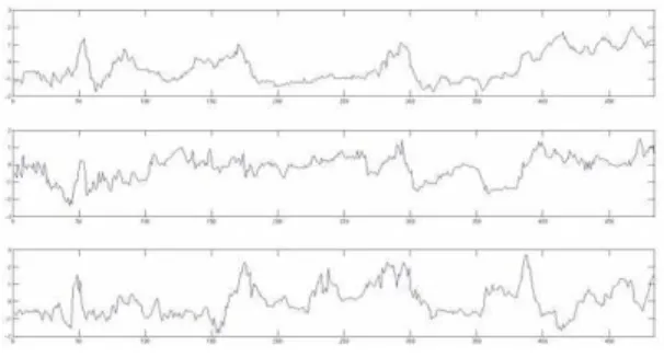
Fig. 2. Sample signal at the top is of high frequency along orientation 0◦.
Sample signal in the middle is of middle frequency along orientation 0◦.
Sample signal at the bottom is of low frequency along orientation 30◦. 1) Data Observations and Assumptions: The algorithm is applied on multidimensional data as each of the 18 dimen-sions of the GIST vector are treated individually. Sample signals are shown in Figure 2. Main variations observed should correspond to significant changes in the structure of the environment. In order to treat those signals, we need to establish an evolution model. We assume that the data follow a normal distribution. This means that the value of the data in each dimension is represented by the mean and a standard deviation representing the signal noise. Moreover, the signals are assumed to be independent.
Assume that µ0is the mean of X1, ..., Xτ and µ1 the mean
of Xτ+1, ..., Xn. µ0 describes the topological place we are
leaving while µ1 describes the topological place we are
entering. τ is the instant and location of the topological place change. Considering the normal distribution of f0 and
f1 with a constant measure noise σ, the uniformly most
powerful test becomes Sτn=
(n − τ + 1)(µ1− µ0)2
2σ2 (6)
This equation mainly describes the detection of a mean shift (µ1− µ0)2 as almost the remaining terms are constants.
τ has no real importance in the equation as the tested τ defines the observations on which µ0 and µ1 are estimated.
Given this observation, the described algorithm aims to detect the mean shifts characterizing the topological place changes.
2) GIST variation detection: State estimation is per-formed using a very simple discrete Kalman model with no control input. The state is measured in a sliding window and modelled as
xn = [µ0,1, ..., µ0,18, µ1,1, ..., µ1,18]t (7)
where µ0,i are the mean computed along each dimension in
the first half of the sliding window and µ1,ithe mean in the
second half. The Kalman model of the system is: (
xn = xn−1+ w
yn = xn+ v
(8)
kiis simply the difference between the two means computed
as ki = µ0,i − µ1,i and is the expression of the mean
shift. While navigating in the same topological place, the parameters are not supposed to change. µ0,i and µ1,ishould
remain constant. The transition state model is then defined with the identity matrix. w is the model error described by a Gaussian noise of null mean. w only comprises the standard deviation in each dimension. We use the value of 0.2 for all µ. v is the measure error described by a Gaussian noise of null mean. v contains the noise standard deviations. Experimentation and observations led to the conclusion that the standard deviations vary between the frequency domains. The values are2.4 for the low frequencies, 3.2 for medium frequencies and3.6 for high frequencies and the thus for µ0,
µ1. All noise standard deviations (w and v) are empirically
estimated on a representative sample of signals. yn
corre-sponds to the observed signals at time n and is the measured state with measure noise added. Kalman filtering (feedback with Kalman gain) is applied on the Kalman model to extract an estimated statexˆn with a minimum of variance.
This system leads to two smoothed curved representing µ0
and µ1. The two curves are finally simply the mean estimate
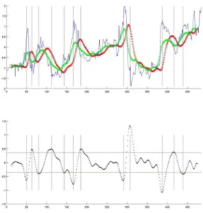
spaced out by half of the sliding window size. As shown in Figure 3, the curves are mixed up when there is no change-point and let appear a delay otherwise. k being the difference between the two curves let appear a peak proportional to the mean shift when there is a change-point. These peaks are then detected and compared with a threshold ν. If the value is greater than ν the peak defines structure change in the environment. The threshold directly impact the sensitivity of the algorithm and so the number of change-points detected. The presented algorithm has the advantage to give the precise
Fig. 3. Top graphic shows the sample signal of middle frequency in orientation 0◦in blue. The green curve is the state estimation in the first half
of the sliding window. The red curve is the state estimation in the second half of the sliding window. The vertical lines are detected change-points. Bottom graphic shows the mean shift k. The red lines are the threshold used. Vertical lines are still the detected change-points when a peak is detected under or over the threshold.
instant of change-point Tc (Neyman-Pearson hypothesis
test-ing) while being as effective as the CUSUM approach. The effectiveness is obtained through the sliding window system for probability density function estimation in the Kalman filter.
Change-points are evaluated along each of the 18 dimen-sions. The drawbacks are irrelevant change-points or many change-points around one location. Irrelevant change-points are due to detection in only a very small subset of the dimensions. The other drawback results from independent evaluation in each dimension. If various signals converge to a change-point, the location of the change-point may vary a little around a mean location. To overcome these drawbacks, we only consider true points as change-points detected in at least 6 dimensions and in close location. 6 dimensions is an experimental evaluation established from the study of the various signals. Considering a true change-point as change-change-points detected in all the dimensions is a nonsense. Each dimension is independent from the computa-tion side. The correlacomputa-tion is only resulting from the structure of the environment. 6 dimensions seems to be a good trade-off between the independence approach of the algorithm and the correlation of the signals due to the environment.
IV. EXPERIMENTALRESULTS
In the following experiments, the sliding window comprises 20 images and the threshold ν was set to0.35.
As the algorithm is designed to run online, computation
time is an important information about the process. All the algorithm is not optimally coded with Matlab. The GIST vector requires around 80ms to be computed. The change-point detection takes less than 10ms most of the time, some peaks to 15ms are observed. The whole process takes around 100ms to detect change-points in the environment. Images can then be processed up to 10Hz which is sufficient for slowly moving robot because there will not be large displacements at high frame rates. An implementation in C++ will lead to a very effective real-time computation allowing online environment segmentation even on fast moving robot with a higher camera frame rate.
A. Indoor Environments
Indoor environments present a great advantage for topological places computation. Places are well defined by rooms and corridors and structure changes are then defined by doors. We tested our algorithm in an indoor environment to validate our approach. Found change-points are easy to compare with doors location.
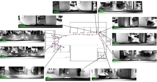
The indoor environment is the Kahn building in the INRIA Sophia-Antipolis research center. The ground plane is shown on Figure 4. The trajectory followed by our robot is overlaid in red on the ground plane. The trajectory starts at the bottom on the right and ends at the bottom on the left. The crosses are the change-points detected by the presented algorithm. Topological places are then defined between two crosses. The first cross is not a real change-point. The detection is due to movements very close to the camera during the robot initialization.
Interestingly, we notice that none of the change-points are located at the door locations but are instead detected before and after door locations. This can be seen on images (406, 751) and (2446, 2731) on Figure 4. From the algorithm side, the door locations themselves are considered as topological places. While not intuitive at first sight, it is very meaningful because they are transitions and are very dissimilar with the environments of both sides. At the door locations, the images are mainly composed of the door uprights and the door itself. A small part comprises the environments from both sides. In terms of orientations and frequencies, the more significant components are orientations of 0◦, representing vertical
edges, in the domain of high frequencies, relating strong edges (door uprights). The door itself is related by low frequencies in any orientation as they are texture-less in our experimentations. Before and after the door location, these orientations and frequencies are less significant because the doorstep represent a small part of the image. Before and after images are then characterized by orientations and frequencies peculiar to each environment type.
Images (2731, 3421) and (4561, 5356) on Figure 4 shows that when the robot comes back on its path, change-points are detected on the same location. Here are examples when the robot enter offices, about-turns and leaves the offices. Moreover, images (2446, 4246) are very spatially close and look very similar. They correspond to images before entering the first office and after leaving it. These images
Fig. 4. Kahn building - Indoor environment.
demonstrate the stability of the detected change-points in the environment. Whatever the path followed by the robot, the change-points are detected on very close locations. Change-points are detected all along the path and some do not correspond to door locations. They are true change-points due to important variations in the perceived environment. Such change-points are illustrated by images 7636 and 7951 on Figure 4. In both images, we can see the same environment. However, the first image seems to describe a place with a lot of space available. The topological place defined between these two change-points is mostly related to this open space. Te second change-points describes a more cluttered place. While the same objects as in the previous change-point are present, we are closer to them. They are of more importance in the perceived environment and have a greater influence in the GIST vector. We then switch from an open space to a cluttered space. This demonstrate that the structure in the perceived environment is an important parameter for environment segmentation. Such kind of segmentation relates the closeness parameter and allows to describe how far away we are from some place.
We had some illumination problems at the bottom on the left of the trajectory resulting in strong intensity variations in the images and even in unexploitable images. Finally, this seems to have a small impact on the topological places detection. The effects are additional change-points and change-points without exact location around the doors. Image 13201 on Figure 4 is an example of this kind of illumination issue.
Figure 5 shows the algorithm robustness to the threshold ν choice and change-points dependence only on environment structure. The tested thresholds are0.6, 0.35 and 0.25. Blue crosses are detected change-points for the three thresholds. Green crosses are detected change-points for threshold 0.35
Fig. 5. Change-points stability over threshold ν.
and 0.25. Black crosses are detected change-points for threshold 0.25. Red crosses are detected change-points for threshold0.35 which have disappeared with threshold 0.25. No change-points disappear switching from threshold0.6 to threshold0.35. As expected with the theory: the lower the threshold, the greater detected change-points number. Very few change-points disappear when lowering the threshold. Changing the threshold value only impacts the number of detected change-points but not their location. This reveals that the algorithm is very robust to change-points location which are really characteristic of the environment.
Disappearance of change-points is due to allowing true change-point detection if at least 6 dimensions converge to change-point detection. For each dimension taken separately, it is impossible to have change-point location variation due to threshold choice. Change-points are well localised in each signal and following the peak value compared to the threshold, they are considered as change-points or not. During the 6 dimensions convergence step, we impose a half sliding window distance between two detected change-points in order to avoid over segmentation and noise sensitivity. If a change-point is detected by lowering the threshold and its distance to the next detected change-point with a higher threshold is inferior to the half sliding window distance, the detected change-point with the higher threshold then disappears. Hopefully, we observe on Figure 5 that there is always black crosses close to the red crosses. This means that disappearing change-points with threshold 0.35 are replaced by very close change-points with threshold0.25.
B. Outdoor Environments
The algorithm was also tested on outdoor environments to prove the validity of our topological place definition. Conversely to indoor environments, change-points are not as well defined as doors. The outdoor environment is the INRIA Sophia-Antipolis campus. A satellite view of the campus is shown in Figure 6. Like for the indoor environment, the trajectory followed by the robot is overlaid in red and the crosses are the detected change-points. The trajectory starts at the bottom and ends at the top of the image.
Images 109, 173 and 205 on Figure 6 show change-point detection while passing in front of a building. Image 109 is while entering the place in front of the building and image 205 is while leaving the place. We could think of a topological place defined between this two images but there is a change-point detected between them and represented by image 173. Determining topological places in outdoor environments is harder than in indoor environments. Never-theless, this change-point is determined by structure change in the environment. In the first image, the place is mainly composed with the building, the small walls and vegetation. In the second image, the wall disappears and let just appear road. In terms of orientations and frequencies, the small wall is made of orientations of90◦
, representing horizontal edges, of high frequencies due to strong edges. The road corresponds to low frequencies in any orientation. The rest of the scene is unchanged. This switch of orientations and frequencies defines this change-point.
Images 347 and 409 represents change-points while entering and leaving a parking. It can be seen from the satellite image that there is a lot of vegetation. Coming back to the purpose of GIST defined by A. Oliva and A. Torralba in [11], there is a switch from naturalness to human made environment for the first change-point and the inverse for the second one. The parking is a human made environment and it is
surrounded by nature. The accessing roads are a small part of the environment in the places before and after the parking. Images 805 and 847 are detected change-points before and after passing under a bridge. While presenting different orientations, this example is very similar to the doorstep case in indoor environments. The images relate very dissimilar environments before and after the bridge.
During this experimentation, strong glares -due to a low al-titude of the sun in the sky- generate important vertical lines of light in the images. Examples are shown in images 409, 631 and 1049 on Figure 6. They sometimes enforce change-point probability of occurrence by adding evidence to weak change-point detections, i.e. change-points detected in less than 6 dimensions. While this adds high vertical frequencies in the image, their impact on the detected change-points is hard to evaluate.
In outdoor environments, it is very hard to evaluate the detected change-points correctness. While some seem to be intuitive like the bridge case or when passing in front of a building, other are very hard to justify. Images 631 and 651 are two detected change-points in front of a building. The first change-point is easy to explain as we are entering the zone in front of the building. The second change-point is hard to justify. We encountered strong glares in this part of the trajectory but we cannot advance that they are responsible of the point. Whereas not showed, the next change-point is also hard to justify. We cannot say at first glance why there are change-points at these locations.
V. CONCLUSION
While indoor environments are studied in [6], [15], [16], [21], [1], [8], [20] and [14], segmentation on outdoor envi-ronments has rarely been studied. Nevertheless, methods like [1] and [8] do not restrict their algorithms to indoor environ-ments and could be applied to outdoor environenviron-ments if the sensed information can be employed. Structure parameters described by the GIST are a valuable representation used in a common approach for indoor and outdoor environments. One drawback of this approach is some sensitivity to illumination changes between the images. Normalisation steps are used and reduce the effects but they are still an issue which consequences are hard to evaluate. In terms of obtained topological maps, the closest results are presented in [8] while their method is based on the graph cuts.
The approach described in this paper allows online environ-ment segenviron-mentation into topological places using very low dimensional data. Approaches using features like SIFT ([14], [20]) require more computation time due to an higher number of features of higher dimension. The presented approach is very efficient using a low dimensional GIST in an simple change-point detection algorithm. It can be easily enhanced to be used at higher frame rates for fast moving robots. Future work will focus on place labelling as GIST was orig-inally designed to categorize environments using machine learning based algorithm. We will study how places are distinguishable and categorizable using our low dimensional GIST. It will allow to determine which orientations and
Fig. 6. INRIA Campus - Outdoor environment.
which frequencies are characteristic of which kind of places. Considering possible labelling process and the change-point location robustness of our algorithm, we aim to integrate it in a larger framework of hierarchical SLAM. Metric level will be performed using [9]. Topological navigation will be a combination of the presented work combined with [2]. Environment segmentation will allow loop closure detection on topological places instead of being performed on im-ages. Loop closure detection will enhance the segmentation process performing place recognition. Already seen places will be inserted in the estimation process of change-point detection improving the change-point location accuracy when coming back to previous places. Semantic level will be based on the labelling ability of this work.
REFERENCES
[1] J. L. Blanco, J. Gonz´alez, and J. A. Fern´andez-Madrigal. Subjective local maps for hybrid metric-topological SLAM. Robotics and Autonomous Systems, 57(1):64–74, 2009.
[2] A. Chapoulie, P. Rives, and D. Filliat. A spherical representation for efficient visual loop closing. In Proceedings of the 11th workshop on
Omnidirectional Vision, Camera Networks and Non-classical Cameras (OMNIVIS 2011), 2011.
[3] J. Courbon, Y. Mezouar, and P. Martinet. Autonomous navigation of vehicles from a visual memory using a generic camera model. Trans.
Intell. Transport. Sys., 10(3):392–402, September 2009.
[4] K. M. G´orski, E. Hivon, A. J. Banday, B. D. Wandelt, F. K. Hansen, M. Reinecke, and M. Bartelmann. Healpix: A framework for high-resolution discretization and fast analysis of data distributed on the sphere. The Astrophysical Journal, 622(2):759, 2005.
[5] L. Itti and P. Baldi. A principled approach to detecting surprising events in video. In CVPR (1), pages 631–637. IEEE Computer Society, 2005.
[6] S. Koenig and R. G. Simmons. Unsupervised learning of probabilistic models for robot navigation. In in Proceedings of the IEEE
Inter-national Conference on Robotics and Automation, pages 2301–2308, 1996.
[7] D. Lowe. Object recognition from local scale-invariant features.
Computer Vision, IEEE International Conference on, 2:1150–1157 vol.2, August 1999.
[8] R. V. Mart´ın, P. N´u˜nez, and A. Bandera. Less-mapping: Online environment segmentation based on spectral mapping. Robotics and
Autonomous Systems, 60(1):41–54, 2012.
[9] M. Meilland, A.I. Comport, and P. Rives. A Spherical Robot-Centered Representation for Urban Navigation. In IEEE/RSJ International
Con-ference on Intelligent Robots and Systems, IROS’10, Taipei, Taiwan, October 2010.
[10] M. Meilland, A.I. Comport, and P. Rives. Dense visual mapping of large scale environments for real-time localisation. In IEEE/RSJ
International Conference on Intelligent Robots and Systems, San Francisco, California, September 25-30 2011.
[11] A. Oliva and A. Torralba. Modeling the shape of the scene: A holistic representation of the spatial envelope. International Journal
of Computer Vision, 42(3):145–175, May 2001.
[12] A. Oliva and A. Torralba. Building the gist of a scene: the role of global image features in recognition. Progress in brain research, 155:23–36, 2006.
[13] A. Ranganathan. PLISS: Detecting and Labeling Places Using Online Change-Point Detection. In Robotics: Science and Systems VI, 2010. [14] A. Ranganathan and F. Dellaert. Bayesian surprise and landmark
detection. In ICRA, pages 2017–2023. IEEE, 2009.
[15] H. Shatkay and L. P. Kaelbling. Learning topological maps with weak local odometric information. In Proceedings of the Fifteenth
international joint conference on Artifical intelligence - Volume 2, pages 920–927, San Francisco, CA, USA, 1997. Morgan Kaufmann Publishers Inc.
[16] A. Tapus and R. Siegwart. Incremental Robot Mapping with Finger-prints of Places. In International Conference on Intelligent Robots
and Systems, pages 172–177, 2005.
[17] G. Tsechpenakis, D. N. Metaxas, C. Neidle, and O. Hadjiliadis. Robust online change-point detection in video sequences. In Proceedings of
the 2006 Conference on Computer Vision and Pattern Recognition Workshop, CVPRW ’06, pages 155–, Washington, DC, USA, 2006. IEEE Computer Society.
[18] L. Vincent. Taking online maps down to street level. Computer, 40:118–120, 2007.
[19] J. Wu, H. I. Christensen, and J. M. Rehg. Visual place categorization: Problem, dataset, and algorithm. In IROS, pages 4763–4770. IEEE, 2009.
[20] Z. Zivkovic, B. Bakker, and B. Krose. Hierarchical map building using visual landmarks and geometric constraints. In Intelligent Robots and
Systems, 2005. (IROS 2005). 2005 IEEE/RSJ International Conference on, pages 2480 – 2485, aug. 2005.
[21] Z. Zivkovic, O. Booij, and B. J. A. Kr¨ose. From images to rooms.