Metal cutting modelling SPH approach

Any correspondence concerning this service should be sent to the repository administrator: staff-oatao@inp-toulouse.fr

O

pen

A

rchive

T

oulouse

A

rchive

O

uverte (

OATAO

)

OATAO is an open access repository that collects the work of Toulouse researchers

and makes it freely available over the web where possible.

This is a publisher-deposited version published in: http://oatao.univ-toulouse.fr/

Eprints ID: 4938

To link to this article: DOI: 10.1504/IJMMM.2011.039645

URL:

http://dx.doi.org/10.1504/IJMMM.2011.039645

To cite this version: LIMIDO Jérôme, ESPINOSA Christine, SALAÜN Michel,

MABRU Catherine, CHIERAGATTI Rémy, LACOME Jean-Luc. Metal cutting

modelling SPH approach. International Journal of Machining and Machinability of

Metal cutting modelling SPH approach

J. Limido*

IMPETUS Advanced Finite Element Analysis, rue du Lanoux, 31330 Grenade sur Garonne, France E-mail: jerome@impetus-afea.com

*Corresponding author

C. Espinosa, M. Salaun, C. Mabru, and

R. Chieragatti

Université de Toulouse, INSA,UPS, Mines Albi, ISAE; Institut Clément Ader, 10 av. Edouard Belin, F-31055 Toulouse, France E-mail: christine.espinosa@isae.fr E-mail: michel.salaun@isae.fr E-mail: catherine.mabru@isae.fr E-mail: remy.chieragatti@isae.fr

J.L. Lacome

31330 Grenade sur Garonne, France E-mail: jll@lstc.com

Abstract: The purpose of this work is to evaluate the use of the smoothed

particle hydrodynamics (SPH) method within the framework of high speed cutting modelling. First, a 2D SPH based model is carried out using the LS-DYNA® software. The developed SPH model proves its ability to account for continuous and shear localised chip formation and also correctly estimates the cutting forces, as illustrated in some orthogonal cutting examples. Then, the SPH model is used in order to improve the general understanding of machining with worn tools. At last, a hybrid milling model allowing the calculation of the 3D cutting forces is presented. The interest of the suggested approach is to be freed from classically needed machining tests: Those are replaced by 2D numerical tests using the SPH model. The developed approach proved its ability to model the 3D cutting forces in ball end milling.

Keywords: high speed machining; smoothed particle hydrodynamics; SPH;

chip formation; tool wear; cutting forces; milling.

Reference to this paper should be made as follows: Limido, J., Espinosa, C.,

Salaun, M., Mabru, C., Chieragatti, R. and Lacome, J.L. (2011) ‘Metal cutting modelling SPH approach’, Int. J. Machining and Machinability of Materials, Vol. 9, Nos. 3/4, pp.177–196.

Biographical notes: Jérôme Limido has experience from research and

advanced engineering within aerospace applications. His main work has focused on processes involving large deformations, both experimentally and numerically. He has special interests in advanced numerical methods (smoothed particle hydrodynamics) and fatigue of materials. He is R&D responsible at IMPETUS Afea France and teaches Advanced Computational Mechanics and Numerical Methods at ISAE.

C. Espinosa, after an A-level diploma in Mathematics-Physics (1982), two licence degrees at the University of Bordeaux I in Theoretical Mathematics and Applied Mathematics (1986), he received his Master degrees at this University (M1 of today Master 1987, M2 1988) in Applied Mathematics. He obtained his PhD in Theoretical and Computational Mechanics (1991) for the development of a non-linear damage anisotropic behaviour for aeronautical composite materials subjected to low velocity impacts. He was hired by DYNALIS in 1992, in charge of LS-DYNA distribution in France. He is an ISAE Associate Professor, for teaching and research in Advanced Computational Mechanics and Numerical Methods.

Michel Salaun teaches mathematics and scientific computing at ISAE. His major field of research is computational mechanics. He developed a mixed finite element for thin elastic shells. This formulation was used for the development of an Eulerian approach for large displacements of thin shells. He works also on numerical modelling of incompressible flows (stream function-vorticity and function-vorticity-velocity-pressure formulations). During the last years, he was interested in the application of extended finite element methods (XFEM) for the modelling of cracks in thin structures, first, in the frame of bidimensionnal linear elasticity and, second, for the Kirchhoff-Love plate model.

Catherine Mabru is an Associate Professor at ISAE. She teaches Elasticity, Thermo-elasticity and Plasticity. Her research mainly deals with fatigue of metallic materials and focuses on the interaction between surface condition and mechanical behaviour. Coupling experimental and numerical approaches, she particularly worked on the effect of machining on fatigue strength and the influence of anodic treatment on thermal fatigue degradation mechanisms of anodic film, both concerning aluminium alloys. Recently, she was interested in studies that aim to isolate surface and subsurface behaviour by analysing thin samples strength under thermo-mechanical fatigue loading.

Remy Chieragatti is an Associate Professor at ISAE. He teaches Fatigue and Mechanics. His research mainly deals with fatigue of metallic materials and focuses on the interaction between surface condition and mechanical behaviour.

Jean Luc Lacome has a background in Applied Mathematics and has been working for the past ten years on the development of smoothed particle hydrodynamics. He has interests in fluid-structure interaction and defence applications.

1 Introduction

Machining is the most used process in industrial components production, while involving very complex fully 3D physical phenomena. A considerable effort has been made by the scientific community to develop accurate theoretical and numerical machining models, each one aiming to represent the relevant phenomena of the physics at the considered scale. Among the objectives of these models reproducing this complexity and linking the quality of the surface to the machine control are often encountered. The focus of this work is to propose a numerical model able to reproduce the efficient cutting physics and quality of the generated surface and link local machining models to the machine driving parameters, in the final goal of predicting the effect of the surface quality on the component fatigue life. The application field is limited here to aeronautical representative samples. To be more precise, the purpose of this work is not to illustrate the use of a (n + 1)th numerical model, nor to represent the whole complexity of the physics in the tool-matter interaction. The originality is to propose a new methodology of machine control to ‘optimise’ in a way the quality of the machined surface regarding fatigue life duration, through the use of an appropriate numerical model, under constraints of being relevant and mechanically consistent with the physics of two mechanical scales. The invisible part of this work is the mathematics, computational mechanics (theory) and code developments (numeric) done prior to the numerical tests. The fatigue life prediction part of the work that uses the numerical tests and the machine driving ‘optimisation’ phase are not presented here.

Why the proposed methodology overcomes the key limitations of existing numerical works? Because numerical models are themselves limited compared to fine theoretical approaches, and due to additional computational and numerical limitations, numerical models are mostly limited to the orthogonal cutting framework, especially when it is aimed to compare numerical results and real complex and uncertain experimental measurements. Thus, 2D plain strain studies are commonly dealt. In these conditions, the full 3D and very complex interacting machine control cutting parameters can be resumed to two of them considered as independent, the cutting speed (Vc) and the feed (f). In that field, most of the numerical models are based on Lagrangian or arbitrary Lagrangian Eulerian finite element methods (ALE FEM). Lists of available publications are of course very large. Taking the risk of not being exhaustive, let us cite only two of them Bil et al. (2004) and Marusich (2001). These references papers in particular show two major difficulties closely related to FEM. First contact and friction models must be introduced thus leading to the necessity of accounting for the thermo-mechanical exchange complexity of machining through the interface description, furthermore a line in 2D. In most cases, the Coulomb model is used. It is very simple to implement and use but the contact complexity is, to us, poorly resituated. Moreover, the friction parameter is shown to be a very sensible coefficient often used to tune the FEM cutting forces on experimental results. Thus, FEM can not be predictive. The workpiece/chip material separation model is the second aspect of the modelling difficulties. Lagrangian based FE methods present the disadvantage of leading to large grid distortions since the matter and the grid are strictly connected in the absence of additional ‘opening’ technique. Use of ALE in the FEM remedy since the matter-grid connection is somewhat relaxed and it allows for the boundary of the matter to evolve while remaining Lagrangian. Remeshing techniques are associated to remapping methods. This is hugely time consuming, and in

order to be not energy dissipative and accurate enough, this implies very fine mesh sizes to follow the matter fluxes that open to question the consistency between the solid continuum mechanics and numerical hypotheses.

Regarding the real 3D industrial machining cases (milling for example), numerical models existing at the beginning of this work are not yet rather powerful because of the huge computing time and still remaining numerical problems. Analytical models are often preferred (Altintas, 2000).

The developed approach is based on the smoothed particle hydrodynamics (SPH) method in the frame of the LS-DYNA® hydrodynamic software (Hallquist, 2006). It is shown in Section 2 that SPH is able to model cutting, avoids the need of contact algorithm or remap/remesh additional techniques. In Section 3, SPH cutting model applications are outlined and compared with other numerical or experimental data. The use of SPH as a numerical tool for a better understanding of the chip formation with worn tools is also presented. Finally, in Section 4, our hybrid (analytic-SPH) 3D milling model is presented. This orthogonal cutting based methodology gives as a result a predicted machined surface geometry without the need of 3D numerical cutting model or real test.

2 SPH cutting model

2.1 Basic principles of the SPH method

SPH method is a meshless Lagrangian technique. Material properties and state variables are approximated by their values on a set of discrete points, or SPH particles. This avoids the severe problems of mesh tangling and distortion which usually occur in Lagrangian analyses involving large deformation. For more details on the method used, the reader can refer to Halquist (2006) and Liu and Liu (2003).

2.2 Model description

Several assumptions were made in order to reduce the model size and the computation time, allowing the development of a useful tool.

The model is implemented in the orthogonal cutting framework, thus in 2D (a 3D model can easily be developed but we will show in Section 4 that a coupled analytical-SPH approach could be more efficient, see Figure 2). The tool is supposed rigid and has an imposed velocity. During the process, the computation time is reduced by using an imposed tool velocity ten times higher than the real velocity. This assumption is usually used in simulation of stamping processes. It is valid as long as the accelerated mass is low and the material behaviour is slightly influenced by the strain rate.

Accurate and reliable flow stress models are highly necessary to represent work material behaviour under high speed cutting conditions. In our model, the constitutive material law proposed by Johnson and Cook (1983) is used and all associated parameters result from the literature.

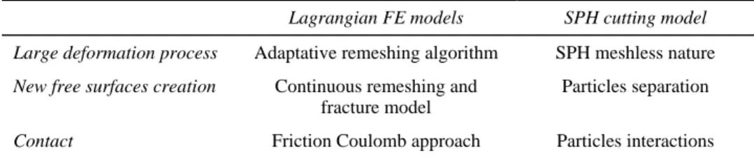
2.3 SPH cutting model capabilities compared to classical FEM approach An overview of the main specificities of the SPH cutting model approach compared to classical Lagrangian FE models is summarised in Table 1.

Table 1 SPH and classical approach comparison

Lagrangian FE models SPH cutting model Large deformation process Adaptative remeshing algorithm SPH meshless nature

New free surfaces creation Continuous remeshing and fracture model

Particles separation

Contact Friction Coulomb approach Particles interactions

SPH method applied to machining modelling involves several advantages.

First, high strains are easily handled. The particles move relatively to each other in a disordered way during the deformation. This can be considered as a particles rearranging without topological restriction, thus no remeshing is needed.

Another advantage induced by SPH is the ‘natural’ chip/workpiece separation. The relative motion of the particles creates the opening. The new free surfaces are given by the particles positions. Thus, the workpiece matter ‘flows naturally’ around the tool tip (Figure 1).

Figure 1 Chip separation (see online version for colours)

Plastic  Deformation  Resultant  Velocity  Piece Tool 

Figure 2 Al6061-T6 Oblique cutting case: 3D SPH model, (a) iso view (b) top view (see online

version for colours)

In the same way, the SPH method presents an original aspect regarding contact handling. Indeed, when a workpiece particle ‘sees’, in its neighbouring, tool particles, then workpiece particle circumvents the tool. Thus, friction is modelled as particles interactions and friction parameter does not have to be defined. SPH friction modelling must be studied in-depth but it offers a very interesting alternative to traditional definitions.

2.4 Some specificities of the SPH model implementation

The implemented SPH model within the framework of LS-DYNA reveals some specific aspects.

Renormalised SPH formulation

Due to the lack of neighbours, classical SPH approximation is not correctly calculated on the boundaries. Indeed, a particle located on a free edge only interacts with existing particles located on one side of the free edge.

LS-DYNA proposes an alternative formulation to particle SPH approximation which corrects this deficiency. This formulation is called renormalisation. It is based on the works of Randles and Libersky (1996) and Vila (2005). The renormalised formulation improves the SPH method consistency (order 1). Two advantages are obtained: a better precision when the particles are disordered and a better approximation of the calculated quantities at the boundary.

In the machining modelling case, standard SPH underestimates the chip curve (Figure 3). The use of the renormalised formulation allows a better modelling of the chip curve and a better evaluation of the matter state on the surface (Figure 3).

Figure 3 Standard/renormalised SPH formulation in metal cutting (see online version for colours)

Standard formulation Renormalised formulation

Numerical instabilities

The SPH method is prone to two types of numerical instabilities: tensile instability and zero energy modes. These aspects are discussed in details in Belytschko and Xiao (2002).

We faced numerical instability of the SPH method for the cutting model. Figure 4 shows an example of numerical fractures. Increasing the physical velocity of the tool

decreases these instabilities. Currently, the SPH method in LS-DYNA does not provide any advanced solution to solve this problem but a work is in progress.

Figure 4 Numerical instabilities (see online version for colours)

V

_V

3 SPH cutting model applications

Two applications are presented here: the first one reproduces a continuous chip process and the second one a shear localised chip. They are studied and compared to experimental results and numerical FEM (AdvantEdge; Marusich, 2001) results. AdvantEdge is a reference in machining simulations. It is an explicit dynamic, thermo-mechanically coupled FEM package specialised for metal cutting. Here, comparisons are carried out on the chip morphology, stress distribution and the specific cutting forces. Other comparisons can be found in Limido et al. (2007).

3.1 Continuous chip: Al6061-T6

We first present the result of a cutting problem using material Aluminium alloy Al6061-T6. The process parameters are defined as follows: speed 10 m/s, rake angle 5 , feed 250 µm and edge radius 25 µm. The material model parameters result from Lesuer (2001). All the AdvantEdge and experimental results presented in this part are based on Marusich (2001).

Chip morphology and stress distribution

LS-DYNA and AdvantEdge chip morphology results are presented in Figure 5. The considered Aluminium alloy produces continuous chip in the speed and feed range studied (Marusich, 2001). LS-DYNA and AdvantEdge models results are in agreement with these experimental observations. The AdvantEdge model overestimates the chip thickness and the LS-DYNA SPH model underestimates it. Figure 5(b) shows the Von Mises stresses during the continuous chip formation. Primary and secondary shear zone can be easily identified.

Figure 5 Al6061-T6, (a) chip thickness AdvantEdge/LS-DYNA comparisons (b) SPH model Von

Mises stress (see online version for colours)

(a) (b)

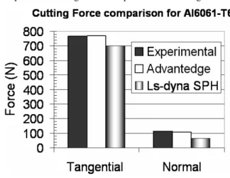
Cutting forces

Normal (or feed) and tangential (or cutting) forces are compared in Figure 6. LS-DYNA predicted cutting forces agree within 10% and 30% of the measured values for tangential and normal components respectively. These differences can be explained by chip separations criteria, friction model and SPH velocity assumption. It is important to recall that the SPH model does not use a numerical friction. Thus the predicted cutting forces are not adjusted. On the other hand, the AdvantEdge model used a Coulomb parameter fixed to 0.2 without any information on how to choose this value.

Figure 6 Al6061-T6 predicted cutting forces comparisons AdvantEdge/LS-DYNA

3.2 Shear localised chip: Ti6Al4V and worn tool

In this section, the Ti6Al4V alloy machining is used under dry conditions. When machining titanium alloys with conventional tools, the tool wear rate progresses rapidly,

and it is generally difficult to achieve a cutting speed of over 60 m/min. The tool wear analysis method developed here is based on a chip formation analysis using experimental and numerical results. The main idea is to use the developed SPH model to study the cutting forces and the chip formation with new and worn tools and compare these results to available experimental data. This work was completed in collaboration with the Lamefip ENSAM Bordeaux France (Limido et al., 2009).

The studied cutting conditions are summarised in Table 2.

Table 2 Cutting conditions

Tool material Tungsten carbides

Grade H13A WC-6Co K20

Rake angle 0

Clearance angle 11

Cutting speed 60 m/min

Feed 0.3 mm

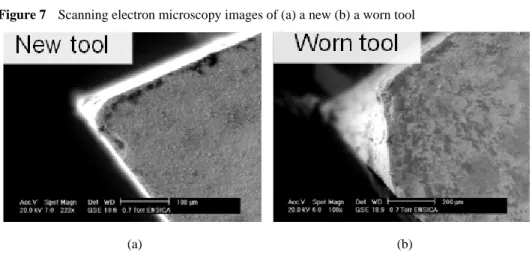
The tool geometry before and after machining are shown in Figure 7.

Figure 7 Scanning electron microscopy images of (a) a new (b) a worn tool

(a) (b)

Chip morphology

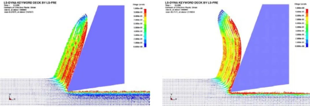
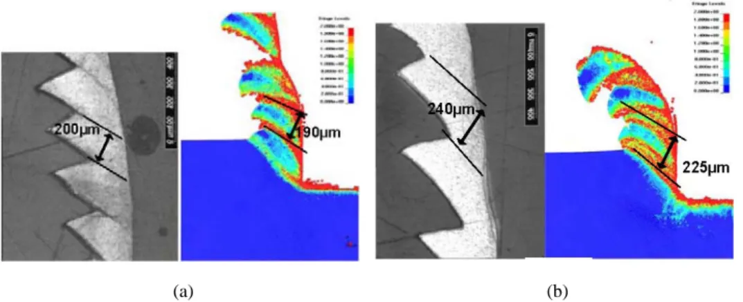
Under the cutting speed and feed range studied, Ti6Al4V alloy produces shear localised chips (see Figure 8). Shear localised chips are characterised by oscillatory profiles. They result from adiabatic shear band formation in the primary shear zone of the workpiece material. The chip type obtained for the SPH model is in accordance with experiments (Figure 8). The SPH model shows a shear band thickness increase and a decrease of frequency of chip segmentation with wear, which is also observed experimentally.

It is possible to identify (Figure 9) a metal dead zone in the chip formation mechanisms with worn tools. This area is reduced to a triangular zone in front of the tool tip which moves with the tool. This physical mechanism was already observed in experiments (Kountanya and Endres, 2001). The SPH approach is able to predict this stagnation zone because of its meshless nature.

Figure 8 Experimental/numerical chip formation using (a) a new (b) a worn tool geometry

(see online version for colours)

(a) (b)

Figure 9 Velocity field at tool tip: metal dead zone identification (see online version for colours)

Y X Workpiece Tool Tip Resultant Velocity Y Component Velocity

Metal Dead Zone

(a) Resultant velocity field (b) Y component velocity field

Cutting forces

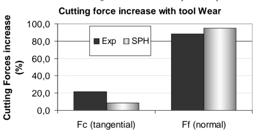
Experimental results, illustrated in Figure 10, show a great influence of wear on the feed force (about 90%) and a less important increase of the cutting force (about 20%). The SPH cutting model results show a mean feed force increase of about 95% with tool wear and of the cutting force of about 10% (Figure 10). So, the SPH model is able to correctly predict these variations, induced by the tool wear by only taking into account the tool tip shape changes. We think that the metal dead zone formed in front of the tool tip is the main cause of the large feed force increase (Limido et al., 2009).

Figure 10 Tool wear influence on cutting forces: SPH model compared to experimental data Cutting force increase with tool Wear

0,0 20,0 40,0 60,0 80,0 100,0 Fc (tangential) Ff (normal) C u tt in g F o rce s i n cr e a se (% ) Exp SPH

4 3D Milling forces via 2D SPH

4.1 Principle of the 3D cutting forces determination

The milling force modelling is not a simple extrapolation of the orthogonal cutting case because locally oblique cutting occurs. Recently, 3D finite elements milling models were developed but the computational times necessary are too important for exploitation within an industrial framework. The alternative suggested here is mainly based on a coupling of Altintas (2000) approach and our 2D SPH model. Altintas approach principle is to consider the total cutting pressures as the sum of the local cutting pressures along the edge(s). In other words, the cutter is represented as a sum of elementary tools.

In the developed model, the local cutting forces are calculated starting from the local cutting conditions (thickness and depth of chip) and from the cutting coefficients by equation (1) (Altintas, 2000). Let us note that tangential components (t index), axial (a index) and radial (r index) of the cutting coefficients are separate in components related to shearing (c index) and in components related to the edge action (e index). The total cutting forces are then determined by integration of the equation (2).

t tc te r rc re a ac ae dF K hdb K ds dF K hdb K ds dF K hdb K ds = + = + = + (1)

dFt, dFr, dFa differential tangential, radial, axial cutting force Ktc, Krc, Kac tangential, radial and axial cutting force coefficients Kte, Kre, Kae tangential, radial and axial edge force coefficients h uncut chip thickness normal to cutting edge

db differential cutting edge length in the direction perpendicular to the cutting velocity

sin sin cos sin cos cos sin sin cos cos cos 0 sin x r y t a z dF k k dF dF k k dF k k dF dF − − − ⎡ ⎤ ⎡ ⎤⎡ ⎤ ⎢ ⎥_{= −}⎢ ₋ ⎥⎢ ⎥ ⎢ ⎥ ⎢ ⎥⎢ ⎥ ⎢ ⎥ ⎢_⎣ − ⎥_{⎦ ⎣}⎢ ⎥_⎦ ⎣ ⎦ ψ ψ ψ ψ ψ ψ (2)

dFx, dFy, dFz differential cutting force components in the workpiece coordinate dFt, dFr, dFa differential tangential, radial, axial cutting force

ψ lag angle in global coordinate, measured from+y-axis CW

k angle in a vertical plane between a point on the flute and the z-axis In order to obtain the total cutting forces by this method, it is necessary to determine on the one hand the local cutting conditions and on the other hand the coefficients of cut. 4.2 Local cutting condition determination

We developed a model which represents the intersection tool/workpiece like the intersection between a B-Rep surface (discretised tool) and a Z-Map volume (discretised workpiece). We chose to use this model in order to determine the local cutting conditions. Indeed, the B-Rep representation of the tool already proposes a discretisation of the cutting edges. Our local ‘tools’ are thus the triangles pairs of discretisation of the total tool. The local cutting conditions are given from the ‘erased’ chip volume by the travel of the local or elementary tool for the considered time step.

Figure 11 Matter removal by an elementary tool of the cutter (see online version for colours)

A

B

C

D

Figure 11 illustrates the cutted chip volume (in red) during a rotation step by the travel of the local tool (in blue). Segment AB represents part of an edge of the total tool at the time t and the segment CD represents this same part of the tool but at next time step t + dt. Exact equation (1) is approximated within the framework of the developed model by equation (3). The total efforts are obtained by summation of the contributions of the elementary tools (i), after projection in the reference workpiece coordinate [equation (4)].

( ) ( ) ( ) chipi ti tci tei i chipi ri rci rei i chipi ai aci aei i V F K K s R z t V F K K s R z t V F K K s R z t = + Δ = + Δ = + Δ ω ω ω (3)

Fti, Fri, Fai tangential, radial, and axial elementary (i) tool force Ktci, Ktei, Krci, Krei, Kaci, Kaei cutting coefficients of an elementary (i) tool Vchipi chip volume removed by the tool (i) during Δt time

step

ω angular tool speed

R(z) tool radius in x-y plane at a point defined by z si elementary (i) tool, cutting edge length

( ) sin sin cos sin cos ( ) cos sin sin cos cos

cos 0 sin ( ) x i i i i i ri y i i i i i ti i i i ai z F k k F F k k F k k F F − − − ⎡ ⎤ ⎡ ⎤ ⎡ ⎤ ⎢ ⎥₌ ⎢_{− −} ⎥ ⎢ ⎥ ⎢ ⎥ ⎢ ⎥ ⎢ ⎥ ⎢ ⎥ ⎢_⎣ − ⎥ ⎢_{⎦ ⎣} ⎥_⎦ ⎣ ⎦

∑

Fti, Fri, Fai tangential, radial, et axial elementary (i) tool force Fx, Fy, Fz cutting force components in the workpiece coordinate

ki angle in a vertical plane between a point on the flute and the z-axis ψi angular position

Figure 12 Developed model compared to Altintas’ (2000) results on a ball-end milling case

The suggested method for determination of the local cutting conditions is very simple (Z-Map+B-Rep). It is thus possible to evaluate the local cutting conditions for various cutting configurations. Nevertheless, analytical solutions exist for ‘simple’ milling conditions like rectilinear slotting (Altintas, 2000). The developed model results are compared (Figure 12) with those of the reference analytical model developed by Altintas (2000). The studied case is related to a rectilinear ball end slotting at constant cutting parameters. We note that the approximation induced by the developed model represents a weak error compared to the reference model (Figure 12). Let us note that the cutting coefficients used for this comparison are those given by Altintas (2000) experiments: Ktc = 2172.1 N/mm2, Krc = 848.90 N/mm2, Kac = –725.07 N/mm2, Kte = 17.29 N/mm, Kre = 7.79 N/mm, Kae = –6.63 N/mm.

4.3 Cutting coefficients identification

The cutting coefficients [equation (1)] are classically determined from many milling tests for which the cutting forces are measured. This approach is known as mechanistic (Altintas, 2000). It permits to obtain very precise results but the determined cutting coefficients are only valid for the considered triplet ‘range, tool, matter’. A simple change like the cutter diameter requires new experimental tests. The predictive character of this approach is thus very limited.

Lee and Altintas (1996) proposed a very interesting alternative to the mechanistic approaches. It permits to determine the cutting coefficients for many cutting conditions only on the basis of orthogonal cutting tests. This approach can be divided into three principal steps summarised here (more precise details can be found in Lee and Altintas, 1996; Altintas, 2000):

• Orthogonal cutting force measurement, cutting and edge force parting, cutting coefficients identification Kte, Kre and Kae [equation (5)].

t tc te tc te r rc re rc re F F F K bh K b F F F K bh K b = + = + = + = + (5)

Ft tangential force (orthogonal cutting) Fr radial force (orthogonal cutting)

Ktc, Krc cutting force coefficient (tangential and radial) Kte, Kre edge force coefficient (tangential and radial)

h uncut chip thickness (feed in orthogonal cutting, also noticed f) b width of cut (also notices w in orthogonal cutting)

The cutting forces are supposed to be linearly dependent on the depth of cut (or feed in orthogonal cutting). Edge forces are identified by extrapolation of the measured data for a null depth of cut (f = 0).

• Identification of the cutting parameters: primary shear band angle [equation (6)], average shearing in the primary shear band [equation (7)], friction angle [equation (8)].

cos arctan 1 sin r c c c r h h h h ⎛ ⎞ ⎜ ⎟ ⎜ ⎟ = ⎜ ₋ ⎟ ⎜ ⎟ ⎝ ⎠ α φ α (6) cos sin sin tc c rc c s c F F bh − = φ φ τ φ (7) arctan rc a r tc F F = + β α (8)

Ft tangential force (orthogonal cutting)

Fr radial force (feed force in orthogonal cutting) h uncut chip thickness (feed in orthogonal cutting) hc cut chip thickness (mean value)

b width of cut αr rake angle

φc primary shear zone angle

τs mean shearing in the primary shear band βa friction angle

• Transformation from orthogonal cutting (2D) to oblique cutting (3D): cutting coefficient identification (9). 2 2 2 2 2 2 2 2 2 2 2

cos( ) sin tan sin _{cos ( ) sin tan}

sin( )

sin cos _{cos ( ) sin tan} cos( ) tan sin tan sin _{cos ( ) sin tan}

s n r n tc c _{c n r n} s n r rc c _{c n r n} s n r n tc c _{c n r n} i K i K i _i i i K i − + = + − + − = + − + − − = + − + τ β α β φ _{φ β α β} τ β α φ _{φ β α β} τ β α β φ _{φ β α β} (9)

Ktc, Krc, Kac cutting coefficients (tangential, radial and axial) φc primary shear band angle

τs mean shear stress in the primary shear band βn normal friction angle (tan βn = tan βa cos i)

αr rake angle

This cutting coefficients definition is obtained on the basis of following simplifying assumption: the angle of the primary shear band in orthogonal cutting is equal to the angle of the primary shear band of oblique cutting; the normal rake angle is equal to the rake angle of orthogonal cutting; the chip flow angle is equal to the angle of obliquity; average shear stress in the primary shear band and the friction coefficient are identical in the orthogonal case and the oblique case.

4.4 From 2D SPH model to 3D oblique cutting

The identification method of the cutting coefficients which we have just presented is classically based on orthogonal cutting experiments results. We propose to replace these physical tests by numerical tests on the basis of model SPH 2D presented in Section 2.

The principal interest is to avoid the numerous orthogonal cutting tests which are necessary when a large variety of tools is studied. Indeed, cutting forces and chip thickness vary, in particular, according to the geometry of the orthogonal cutting tool (edge radius, rake angle). However, we showed into Section 2 that 2D SPH model permits to correctly take into account the tool geometry effect on the cutting forces. Thus, it seems interesting to replace the experimental phase of the cutting coefficients identification by a numerical SPH phase.

This suggested approach is evaluated in the following via the cutting coefficient identification in the case of aluminium 7075-T6 alloy.

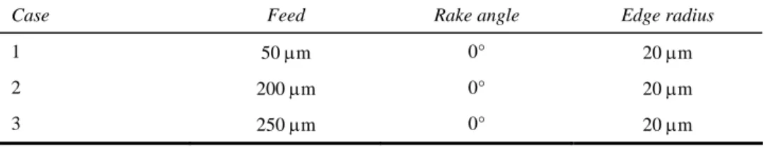
SPH Model was used in order to determine the cutting forces and the chip thickness for 3 different depths of cut (or feed) (Table 3). The JC material model parameters used result from work of Fang and Fronk (2007) (Table 4).

Table 3 Cutting parameters

Case Feed Rake angle Edge radius

1 50 μm 0° 20 μm

2 200 μm 0° 20 μm

3 250 μm 0° 20 μm

Table 4 JC model parameters

A B n C m

496 MPa 310 MPa 0.3 0.0 1.2

Source: Fang and Fronk (2007)

Obtained SPH Results are gathered in Figure13. The equations of the linear regression curves represented in grey permits to obtain Kte = 15 N/mm and Kre = 29N/mm. Kae is often negligible and fixed at a zero value (Lee and Altintas, 1996). Equations (6), (7) and (8) permit to obtain the Table 5 values.

Equation (9) gives the three cutting coefficients Ktc, Krc, Kac. Let us note that these coefficients vary according to the helix angle (i) as illustrated in Figure 14.

Figure 13 Cutting forces predicted by SPH 2D model, α = 0 r = 20 μm AA7075-T6

Table 5 Orthogonal cutting characteristic parameters

Shear angle

φc ( )

Mean shear stress

τs (MPa)

Friction angle

βa ( )

33.7 375 38.7

Figure 14 Cutting coefficient evolution with helix angle (see online version for colours)

0 5 10 15 20 25 30 0 200 400 600 800 1000 1200 i (°) N /mm² Ktc Krc Kac

Validation of the cutting forces 3D model

We validate the proposed approach by comparison to a reference case resulting from Lamikiz et al. (2004) work. This case corresponds to a 7075-T6 aluminium alloy ball-end milling of a slope with a 15° angle (Figure 15). The cutting condition studied is defined by the Table 6. The 3D model results are based on the cutting coefficients determined via the 2D SPH model (Figure 14).

The numerical and experimental results obtained by Lamikiz et al. (2004) are compared with those of the 3D model developed, see Figure 16. We can note that our model permits to obtain comparable results to the Lamikiz model. Maximum obtained error compared to the tests is approximately 25% for the studied case. This one corresponds to the Fy component and we can notice that this error is weaker for the Fx and Fz components.

Figure 15 Machining strategy of the studied case

15° 

Table 6 Validation case definition

Mill Radius R0 Flutes number Nf Helix angle i0 Feed f Depth of cut Ap Ball-end 4 mm 2 30 0.15 mm/dent 2mm

Figure 16 3D model validation (see online version for colours)

Let us note that the input data necessary to the implementation of the 3D milling forces calculation are limited to the geometrical definition of the cutter, the machining parameters and the JC material model parameters for considered alloy. The developed approach thus permits to limit in a very important way the quantity of needed tests.

It is possible to use this model in order to evaluate the tool geometry influence on the cutting forces. An example concerning the tool radius influence in the case of a plane milling is illustrated in Figure 17. We note that the normal force on the generated surface (Fz) is very influenced by the ball-end tool radius. It would be possible to study the influence of each geometrical parameter for a tool family, as well as the influence of the machining conditions. Thus, determining optimum machining conditions could be possible, but that exceeds the framework of this study.

Figure 17 Tool radius effect on milling forces (model results) (see online version for colours)

5 Conclusions

The results of the LS-DYNA SPH model were compared with experimental and numerical data. This study shows the relevance of the selected numerical tool. The SPH model is able to predict continuous and shear localised chips. The model also correctly estimates the cutting forces without introducing an adjusting friction parameter. Thus, comparable results compared to machining dedicated codes are obtained.

The SPH 2D cutting model has also been implemented as a helpful tool for understanding chip formation. The meshless nature of the method makes possible to represent a dominating physical phenomenon in the chip formation with strongly worn tool: the metal dead zone.

We also validated a 3D hybrid milling force model that couple our 2D SPH model and a semi-analytical model. This hybrid model permits to study industrial cases without building a 3D large and time consuming numerical model. It could be interesting to include our approach in a machining strategy optimisation study.

References

Altintas, Y. (2000) Manufacturing Automation-Metal Cutting Mechanics Machine Tool Vibrations

and CNC Design, Cambridge University Press.

Belytschko, T. and Xiao, S. (2002) ‘Stability analysis of particle methods with corrected derivatives’, Computers & Mathematics with Applications, Vol. 43, pp.329–350.

Bil, H., Engin, S. and Erman A. (2004) ‘A comparison of orthogonal cutting data from experiments with three different finite element models’, International Journal of Machine Tools and

Manufacture, Vol. 44, pp.933–944.

Fang, N. and Fronk, T.H. (2007) ‘Method for modeling material constitutive behavior’, US Patent 7-240 562 B.

Halquist, J.O. (2006) LS-DYNA Theory Manual, ISBN 069778540-0-0.

Johnson, G.R. and Cook, W.H. (1983) ‘A constitutive model and data for metals subjected to large strains, high strain rates and high temperatures’, in Proceedings of the 7th International

Kountanya, R.K. and Endres, W.J. (2001) ‘A high-magnification experimental study of orthogonal cutting with edge-honed tools’, Proceedings of ASME International Mechanical Engineering

Congress and Exposition.

Lamikiz, A., Lopez de Lacalle, L.N., Sanchez, J.A. and Salgado, M.A. (2004) ‘Cutting force estimation in sculptured surface milling’, International Journal of Machine Tools and

Manufacture, Vol. 44, pp.1511–1526.

Lee, P. and Altintas, Y. (1996) ‘Prediction of ball-end milling forces from orthogonal cutting data’,

International Journal of Machine Tool Manufacture, Vol. 36, pp.1059–1072.

Lesuer, D.R. (2001) ‘Experimental investigations of material models for Ti-6AL-4V titanium and 2024-T3 aluminum’, Technical Report DOT/FAA/AR-00/25, U.S. Department of Transportation Federal Aviation Administration.

Limido, J., Calamaz, M., Espinosa, C., Nouari, M., Salaün, M., Girot, F. and Coupard, D. (2009) ‘Toward a better understanding of tool wear effect through a comparison between experiments and numerical model’, International Journal of Refractory Metals and Hard Materials, Vols. 27–3, pp.595–604.

Limido, J., Espinosa, C., Salaun, M. and Lacome, J.L. (2007) ‘SPH method applied to high speed cutting modelling’, International Journal of Mechanical Sciences, Vol. 49, pp.898–908. Liu, G.R. and Liu, M.B. (2003) ‘Smoothed particle hydrodynamics: a meshfree particle method’,

World Scientific.

Marusich, T.D. (2001) ‘Effects of friction and cutting speed on cutting force’, ASME MED-23313, pp.115–138.

Randles, P. and Libersky, L. (1996) ‘Smoothed particle hydrodynamics: some recent developments and applications’, Comput. Meths. Appl. Mech. Engrg., Vol. 139, pp.375–408.

Vila, J.P. (2005) ‘SPH renormalized hybrid methods for conservation laws: applications to free surface flows’, Lectures Notes in Computational Science and Engineering, Vol. 43, pp.207–229.