O
pen
A
rchive
T
OULOUSE
A
rchive
O
uverte (
OATAO
)
OATAO is an open access repository that collects the work of Toulouse researchers and
makes it freely available over the web where possible.
This is an author-deposited version published in :
http://oatao.univ-toulouse.fr/
Eprints ID : 12877
URL:
http://dx.doi.org/10.1007/978-3-642-40885-4_10
To cite this version :
Balbiani, Philippe and Mikulás, Szabolcs Decidability
and complexity via mosaics of the temporal logic of the lexicographic
products of unbounded dense linear orders. (2013) In: 9th International
Symposium Frontiers of Combining Systems (FroCoS), 18 September 2013 -
20 September 2013 (Nancy, France).
Any correspondance concerning this service should be sent to the repository
administrator:
[email protected]
Decidability and Complexity via Mosaics
of the Temporal Logic of the Lexicographic
Products of Unbounded Dense Linear Orders
Philippe Balbiani1 and Szabolcs Mikul´as2
1 Institut de recherche en informatique de Toulouse, CNRS — University
of Toulouse, 118 Route de Narbonne, 31062 Toulouse CEDEX 9, France [email protected]
2 Department of Computer Science and Information Systems, Birbeck — University
of London, Malet Street, London WC1E 7HX, UK [email protected]
Abstract. This article considers the temporal logic of the lexicographic products of unbounded dense linear orders and provides via mosaics a complete decision procedure in nondeterministic polynomial time for the satisfiability problem it gives rise to.
Keywords: Linear temporal logic, lexicographic product, satisfiability problem, decidability, complexity, mosaic method, decision procedure.
1
Introduction
The mosaic method originates in algebraic logic, see [19], where the existence of a model is proved to be equivalent to the existence of a finite set of partial models verifying some conditions. It has also been applied for proving complete-ness and decidability of temporal logics over linear flows of time. See [5, section 6.4], or [7, 16, 17, 20]. For their use, specialized systems such as temporal logics must be combined with each other. This has led to the development of tech-niques for the combination of linear flows of time such as the classical operation of Cartesian product [10, 11, 14, 21]. Within the context of modal logic, the operation of lexicographic product of Kripke frames has been introduced as a variant of the operation of Cartesian product. It has also been used for defining the semantical basis of different languages designed for time representation and temporal reasoning from the perspective of non-standard analysis. See [1–3].
In [3], the temporal logic of the lexicographic products of unbounded dense lin-ear orders has been considered and its complete axiomatization has been given. The purpose of this paper is to apply the mosaic method for providing a com-plete decision procedure in nondeterministic polynomial time for the satisfiability problem this temporal logic gives rise to. Its section-by-section breakdown is as follows. Section 2 formally introduces the lexicographic products of unbounded dense linear orders and presents the syntax and the semantics of the tempo-ral logic we will be working with. Sections 3 defines mosaics and collections
of mosaics satisfying saturation properties. In Section 4 and 5, we prove the completeness and soundness, respectively, of the mosaic method. Applying these result we prove in Section 6 that the satisfiability problem for our temporal logic is decidable in nondeterministic polynomial time.
2
Products of Unbounded Dense Linear Orders
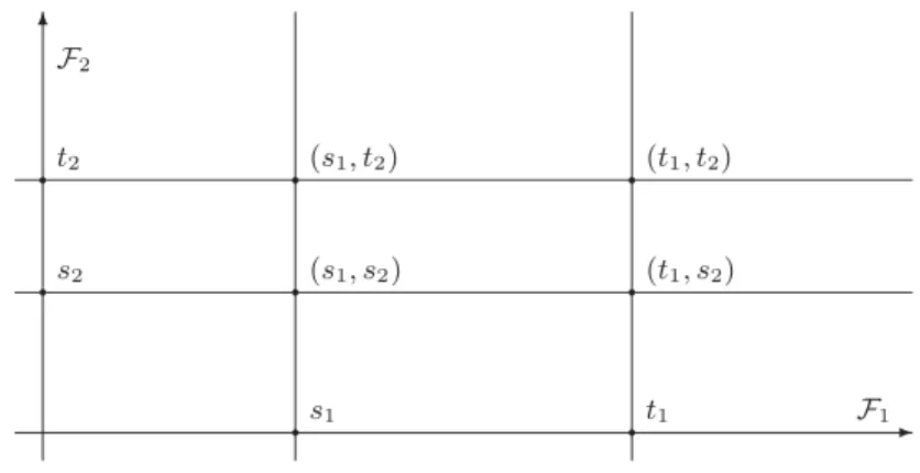
Let F1 = (T1, <1) and F2 = (T2, <2) be linear orders. Their lexicographic
prod-uct is the strprod-ucture F = (T, ≺1, ≺2) where
– T = T1× T2,
– ≺1and ≺2are binary relations on T defined by (s1, s2) ≺1(t1, t2) iff s1<1t1
and (s1, s2) ≺2(t1, t2) iff s1= t1 and s2<2t2.
We define the binary relation ≺ on T by (s1, s2) ≺ (t1, t2) iff (s1, s2) ≺1(t1, t2)
or (s1, s2) ≺ (t1, t2). The effect of the operation of lexicographic product may be
described informally as follows: given two linear orders, their lexicographic prod-uct is the strprod-ucture obtained by replacing each point of the first one by a copy of the second one. The global intuitions underlying such an operation is based upon the fact that, depending on the accuracy required or the available knowledge, one can describe a temporal situation at different levels of abstraction. See [4, section I.2.2], or [8] for details. In Fig. 1 below, we have s1 <1 t1 and s2 <2 t2.
As a result, we have (s1, s2) ≺2 (s1, t2), (s1, s2) ≺1 (t1, s2), (s1, s2) ≺1 (t1, t2),
(s1, t2) ≺1 (t1, s2), (s1, t2) ≺1 (t1, t2) and (t1, s2) ≺2 (t1, t2). It is now time to
meet the temporal language we will be working with. Let At be a countable set of atomic formulas (with typical members denoted p, q, etc). We define the set Lt of formulas of our temporal language (with typical members denoted ϕ, ψ,
etc.) as follows: – ϕ := p | ⊥ | ¬ϕ | (ϕ ∨ ψ) | G1ϕ | G2ϕ | H1ϕ | H2ϕ, ✲ F1 ✻ F2 q s1 q t1 q s2 q t2 q (s1, s2) q (t1, s2) q (s1, t2) q (t1, t2)
the formulas G1ϕ, G2ϕ, H1ϕ and H2ϕ being read “ϕ will be true at each point
within the future of but not infinitely close to the present point”, “ϕ will be true at each instant within the future of and infinitely close to the present instant”, “ϕ has been true at each point within the past of but not infinitely close to the present point” and “ϕ has been true at each point within the past of and infinitely close to the present point”. We adopt the standard definitions for the remaining Boolean connectives. As usual, we define for all i ∈ {1, 2},
– Fiϕ := ¬Gi¬ϕ,
– Piϕ := ¬Hi¬ϕ,
– ✸iϕ := ϕ ∨ Fiϕ ∨ Piϕ.
The notion of a subformula is standard. It is usual to omit parentheses if this does not lead to any ambiguity. The size of a formula ϕ, in symbols |ϕ|, is the number of symbols of ϕ. A model is a structure M = (F1, F2, V ) where F1= (T1, <1)
and F2 = (T2, <2) are linear orders and V : At → ℘(T1× T2) is a valuation.
Satisfaction is a ternary relation |= between a model M = (F1, F2, V ), a pair
(s1, s2) ∈ T1× T2 and a formula ϕ. It is defined by induction on ϕ as usual. In
particular, for all i ∈ {1, 2},
– M, (s1, s2) |= Giϕ iff M, (t1, t2) |= ϕ for every (t1, t2) ∈ T1× T2 such that
(s1, s2) ≺i(t1, t2),
– M, (s1, s2) |= Hiϕ iff M, (t1, t2) |= ϕ for every (t1, t2) ∈ T1× T2 such that
(t1, t2) ≺i(s1, s2).
As a result, for all i ∈ {1, 2},
– M, (s1, s2) |= Fiϕ iff M, (t1, t2) |= ϕ for some (t1, t2) ∈ T1× T2 such that
(s1, s2) ≺i(t1, t2),
– M, (s1, s2) |= Piϕ iff M, (t1, t2) |= ϕ for some (t1, t2) ∈ T1× T2 such that
(t1, t2) ≺i(s1, s2),
– M, (s1, s2) |= ✸2ϕ iff M, (s1, t) |= ϕ for some t ∈ T2.
M is said to be a model for ϕ iff there exists (s1, s2) ∈ T1 × T2 such that
M, (s1, s2) |= ϕ. In this case, we shall also say that ϕ is satisfied in M. Let
C1 and C2 be classes of linear orders. We shall say that a formula ϕ is
satis-fiable with respect to (C1, C2) iff there exists a linear order F1 = (T1, <1) in
C1, there exists a linear order F2 = (T2, <2) in C2 and there exists a valuation
V : At → ℘(T1×T2) such that (F1, F2, V ) is a model for ϕ. The temporal logic of
(C1, C2) is the set of all formulas ϕ such that ¬ϕ is not satisfiable with respect to
(C1, C2). The class of all unbounded dense linear orders will be denoted Cud. [3]
considers the temporal logic of (Cud, Cud) and gives its complete axiomatization.
The satisfiability problem of this temporal logic is to
– determine whether a given formula ϕ is satisfiable with respect to (Cud, Cud).
In order to provide a complete decision procedure in nondeterministic polynomial time for it, we use mosaics.
3
Mosaics
Until the end of this paper, ξ will denote a fixed formula and Γ will denote the least set of formulas such that ✸2ξ ∈ Γ (recall that ✸2ϕ is defined as
ϕ ∨ F2ϕ ∨ P2ϕ) and ⊤ ∈ Γ , Γ is closed under subformulas and single negations
(we identify ¬¬γ with γ) and
– if G1ϕ ∈ Γ or H1ϕ ∈ Γ , then G2ϕ, H2ϕ ∈ Γ ,
– if F1ϕ ∈ Γ or P1ϕ ∈ Γ , then ✸2ϕ ∈ Γ .
Recall that ξ has at most |ξ| subformulas. Closing this set under single nega-tions gives us at most 2 × |ξ| formulas. Then ✸2ξ yields 2 × |ξ| + 10
formu-las (subformuformu-las and their negations). The first requirement above introduces at most 2 new formulas plus their negations, and the last requirement intro-duces at most 10 new formulas (with negations), for every ϕ. Thus we get that |Γ | ≤ 14 × (2 × |ξ| + 10) + 2 (the 2 is for ⊤ and ⊥).
Let λ be a function such that dom(λ) ⊆ Γ is closed under single negations and ran(λ) ⊆ {0, 1}. We say that λ is adequate if
– ⊤ ∈ dom(λ) and λ(⊤) = 1,
– for every γ ∈ dom(λ), we have λ(¬γ) = 1 − λ(γ),
– for every γ ∨ρ ∈ dom(λ), we have λ(γ ∨ρ) ≥ λ(γ) provided that γ ∈ dom(λ), λ(γ ∨ ρ) ≥ λ(ρ) provided that ρ ∈ dom(λ), and λ(γ ∨ ρ) = max{λ(γ), λ(ρ)} if both γ, ρ ∈ dom(λ).
The reason for the complicated form of the last condition is that generally we do not require that dom(λ) is closed under subformulas. However, when we state a requirement that λ(γ) ∈ {0, 1}, then we implicitly require that γ ∈ dom(λ). Definition 1. Let i ∈ {1, 2} and (σ, τ ) be a pair of adequate functions. We define the following coherence properties.
Gi-coherence σ(Giϕ) = 1 implies τ (Giϕ) = τ (ϕ) = 1.
Hi-coherence τ (Hiϕ) = 1 implies σ(Hiϕ) = σ(ϕ) = 1.
1. A1-mosaic is a pair (σ, τ ) such that σ and τ are adequate functions, (σ, τ ) satisfiesG1- and H1-coherence and the following transfer conditions.
G-transfer σ(G1ϕ) = 1 implies τ (G2ϕ) = τ (H2ϕ) = 1.
H-transfer τ (H1ϕ) = 1 implies σ(G2ϕ) = σ(H2ϕ) = 1.
2. A2-mosaic is a pair (σ, τ ) such that σ and τ are adequate functions with full domain dom(σ) = dom(τ ) = Γ , (σ, τ ) satisfies G2- and H2-coherence and
the following uniformity conditions. G1-uniformity σ(G1ϕ) = τ (G1ϕ).
H1-uniformity σ(H1ϕ) = τ (H1ϕ).
As an example of mosaics take a model M = (F1, F2, V ) with unbounded,
℘(T1× T2). Denote T := T1× T2. Define for every (s, t) ∈ T , λ(s,t): Γ → {0, 1} by λ(s,t)(γ) := ( 1 if M, (s, t) |= γ 0 otherwise (1)
for every γ ∈ Γ . It is straightforward to check that
– for every (s, t), (u, v) ∈ T with s <1u, the pair (λ(s,t), λ(u,v)) is a 1-mosaic
(with full domain)
– for every (s, t), (s, u) ∈ T with t <2u, the pair (λ(s,t), λ(s,u)) is a 2-mosaic.
For every s ∈ T1, define κs as follows:
κs(γ) :=
1 if λ(s,u)(γ) = 1 for every u ∈ T2
0 if λ(s,u)(γ) = 0 for every u ∈ T2
undefined otherwise
(2)
for every γ ∈ Γ . Then κs is an adequate function and (κs, κt) is a 1-mosaic
whenever s <1t. An i-SSM will correspond to a flow of time in dimension i.
Definition 2. Let i ∈ {1, 2}. An i-saturated set of mosaics, an i-SSM, is a collection M of i-mosaics such that M satisfies the Density, No-endpoints and the corresponding i-saturation conditions below.
Density If (σ, τ ) ∈ M , then there is µ such that (σ, µ), (µ, τ ) ∈ M .
No-endpoints If (σ, τ ) ∈ M , then there are µ, ν such that (µ, σ) ∈ M and (τ, ν) ∈ M .
F1-saturation—insertion If(σ, τ ) ∈ M , σ(F1ϕ) = 1 and τ (F1ϕ) = τ (✸2ϕ) =
0, then there is µ such that µ(✸2ϕ) = 1 and (σ, µ), (µ, τ ) ∈ M .
F2-saturation—insertion If (σ, τ ) ∈ M , σ(F2ϕ) = 1 and τ (F2ϕ) = τ (ϕ) = 0,
then there isµ such that µ(ϕ) = 1 and (σ, µ), (µ, τ ) ∈ M .
P1-saturation—insertion If(σ, τ ) ∈ M , τ (P1ϕ) = 1 and σ(P1ϕ) = σ(✸2ϕ) =
0, then there is µ such that µ(✸2ϕ) = 1 and (σ, µ), (µ, τ ) ∈ M .
P2-saturation—insertion If(σ, τ ) ∈ M , τ (P2ϕ) = 1 and σ(P2ϕ) = σ(ϕ) = 0,
then there isµ such that µ(ϕ) = 1 and (σ, µ), (µ, τ ) ∈ M .
F1-saturation—expansion If (σ, τ ) ∈ M and τ (F1ϕ) = 1, then there is µ
such thatµ(✸2ϕ) = 1 and (τ, µ) ∈ M .
F2-saturation—expansion If (σ, τ ) ∈ M and τ (F2ϕ) = 1, then there is µ
such thatµ(ϕ) = 1 and (τ, µ) ∈ M .
P1-saturation—expansion If (σ, τ ) ∈ M and σ(P1ϕ) = 1, then there is µ
such thatµ(✸2ϕ) = 1 and (µ, σ) ∈ M .
P2-saturation—expansion If (σ, τ ) ∈ M and σ(P2ϕ) = 1, then there is µ
such thatµ(ϕ) = 1 and (µ, σ) ∈ M .
That is, besides the Density and No-endpoint conditions, a 1-SSM should satisfy the F1-saturation and P1-saturation conditions and a 2-SSM should satisfy the
there is (µ, ν) ∈ M such that µ(ϕ) = 1 or ν(ϕ) = 1. Let us continue with our example. The collections
{(λ(s,t), λ(u,v)) : (s, t) ≺1(u, v)} and {(κs, κu) : s <1u}
of 1-mosaics are 1-SSMs. Fix s ∈ T1and consider the set Msof 2-mosaics defined
by
Ms:= {(λ(s,t), λ(s,u)) : t, u ∈ T2, t <2u}.
It is easy to check that Msis a 2-SSM for every s ∈ T1. A 1-supermosaic will be
a 1-mosaic of two 2-SSMs.
Definition 3. Let M be a 2-SSM. We define λM by
λM(γ) := 1 ifµ(γ) = ν(γ) = 1 for every (µ, ν) ∈ M 0 ifµ(γ) = ν(γ) = 0 for every (µ, ν) ∈ M undefined otherwise (3)
for every γ ∈ Γ . Observe that λM is an adequate function.
A1-supermosaic is a pair (M, N ) of 2-SSMs such that (λM, λN) is a 1-mosaic.
In our example, for every s, t ∈ T1 such that s <1 t, the pair (Ms, Mt) is a
1-supermosaic. A saturated set of 1-supermosaics will correspond to a flow (in dimension 1) of flows (in dimension 2).
Definition 4. A saturated set of 1-supermosaics, a 1-SSS, is a collection Σ of 1-supermosaics such that {(λM, λN) : (M, N ) ∈ Σ} is a 1-SSM.
We say that Σ is a 1-SSS for ϕ if there is (M, N ) ∈ Σ such that λM(✸2ϕ) = 1
or λN(✸2ϕ) = 1. Observe that then there is a mosaic (σ, τ ) in one of the
2-SSMs in one of the 1-supermosaics of Σ such that σ(ϕ) = 1 or τ (ϕ) = 1. In our example the set
ΣM:= {(Ms, Mt) : s, t ∈ T1, s <1t}
is a 1-SSS and in fact a 1-SSS for ξ if there is (s, t) ∈ T1×T2such that M, (s, t) |=
ξ. Our running example should convince the reader that satisfiability of ξ implies the existence of a 1-SSS for ξ. But we want to be more economical in creating the 1-SSS; we will describe the procedure for creating a smaller 1-SSS in Section 5. First we show how to create a model from a 1-SSS, though.
4
Completeness
In this section we show the completeness of the mosaic approach. We will need the following.
Definition 5. Let i ∈ {1, 2} and W = (W, <, λ) be a structure such that (W, <) is a linear order and λq is an adequate function for every q ∈ W . We say that
W is i-consistent if it satisfies for every q ∈ W , the corresponding i-completness and i-soundness conditions below.
Gi-soundness Ifλq(Giγ) = 1, then λp(Giγ) = λp(γ) = 1 for every p ∈ W such
thatq < p.
Hi-soundness Ifλq(Hiρ) = 1, then λp(Hiρ) = λp(ρ) = 1 for every p ∈ W such
thatp < q.
F1-completeness If λq(F1γ) = 1, then there is p ∈ W such that q < p and
λp(✸2γ) = 1.
F2-completeness If λq(F2γ) = 1, then there is p ∈ W such that q < p and
λp(γ) = 1.
P1-completeness If λq(P1ρ) = 1, then there is p ∈ W such that p < q and
λp(✸2γ) = 1.
P2-completeness If λq(P2ρ) = 1, then there is p ∈ W such that p < q and
λp(γ) = 1.
That is, a 1-consistent structure must satisfy the G1-soundness, H1-soundness,
F1-completeness and P1-completeness conditions, and a 2-consistent structure
satisfies the G2-soundness, H2-soundness, F2-completeness and P2-completeness
conditions.
Let W = (W, <, λ) be a structure such that (W, <) is a linear order and λq is
an adequate function for every q ∈ W . A future defect of W is a pair (q, γ) such that λq(Fiγ) = 1 but there is no p > q such that λpsatisfies the requirements in
the Fi-completeness condition above. Past defects are defined similarly. Below
we will construct a i-complete (i.e., without defects) and i-sound structure from an i-SSM, see Case 1 and 2 in the proof of Lemma 1 below, where we construct the required future and past witnesses for the defects. In addition, we need that the constructed structure is dense and without endpoints. That is why we will need Case 3 and 4, where we construct new successors and predecessors for each point in the linear order, which in the limit of the construction yields a dense linear order without endpoints.
Lemma 1. Let i ∈ {1, 2}. Assume that M is an i-SSM for ϕ. Then there is an i-consistent structure QM = (QM, <, λ) such that (QM, <) is isomorphic to the
rationals Q and λq(ϕ) = 1 for some q ∈ QM.
Proof. We will define the order (QM, <) and the adequate functions λq by
in-duction. To this end let us have a countable enumeration D of potential defects {(q, γ, k) : q ∈ Q, γ ∈ Γ, k ∈ {1, 2, 3, 4}} such that every item appears infinitely often. The value of k will indicate the type of the potential defect: future, past, successor, predecessor.
By assumption there is an i-mosaic (µ, ν) ∈ M such that µ(ϕ) = 1 or ν(ϕ) = 1. In the base step of the construction we define the finite order Q1= {0, 1} with
0 < 1 and functions λ0 = µ and λ1 = ν. Obviously the soundness conditions
restricted to Q1 hold.
For the inductive step assume that we constructed a sound structure Qn consisting of a finite order (Qn, <) = (q0 < q1 < . . . < qn) and
ade-quate functions λq for q ∈ Qn such that (λqj, λqj+1) ∈ M for every j < n.
Let D(n) = (q, γ, k). If q /∈ Qn, then we define Qn+1:= Qn. Otherwise we
con-sider the following four cases. If none of the four cases below holds, then we let Qn+1:= Qn.
Case 1 k = 1, λq(Fiγ) = 1 and for every r ∈ Qnwith q < r, we have λr(✸2γ) =
0 in case i = 1, or λr(γ) = 0 in case i = 2.
We will construct the required witness in the future of q. First assume that for every r with q < r, we have λr(Fiγ) = 1 (note that this includes the case
q = qn). The i-mosaic (λqn−1, λqn) ∈ M . By Fi-saturation—expansion there
is an i-mosaic (λqn, µ) ∈ M such that
– µ(✸2γ) = 1 if i = 1
– µ(γ) = 1 if i = 2.
In this case we define (Qn+1, <) := (q0< q1< . . . < qn< p) for some p ∈ Q
such that qn< p and let λp:= µ. Next assume that there is r with q < r such
that λr(Fiγ) = 0. Let m be such that qm is minimal in Qn with respect to
this property. Consider the i-mosaic (λqm−1, λqm) ∈ M . By Fi-saturation—
insertion there is an adequate function µ such that (λqn−1, µ), (µ, λqn) ∈ M
and
– µ(✸2γ) = 1 if i = 1
– µ(γ) = 1 if i = 2.
Then we let (Qn+1, <) := (q0< . . . < qm−1< p < qm< . . . < qn) for some
p ∈ Q such that qm−1< p < qm and define λp:= µ.
Case 2 k = 2, λq(Piγ) = 1 and for every r ∈ Qnwith r < q we have λr(✸2γ) =
0 if i = 1, or λr(γ) = 0 if i = 2.
A completely analogous construction to Case 1 provides the required witness in the past of q.
Case 3 k = 3.
We will construct a new successor for q. In the case q = qn, consider
(λqn−1, λqn) ∈ M . By the No-endpoints condition, we have an i-mosaic
(λqn, µ) ∈ M . We define (Qn+1, <) := (q0 < q1 < . . . < qn < p) for some
p ∈ Q such that qn < p and let λp := µ. Now assume that q = qm < qn.
Consider the i-mosaic (λqm, λqm+1) ∈ M . Then there is an adequate function
µ such that (λqm, µ), (µ, λqm+1) ∈ M , by the Density condition. Then we let
(Qn+1, <) := (q0< . . . < qm< p < qm+1 < . . . < qn) for some p ∈ Q such
that qm−1< p < qm and define λp:= µ.
Case 4 k = 4.
A completely analogous construction to Case 3 provides a new predecessor of q.
It is easy to check that Qn+1 is sound in every case, since it consists of elements
of M . Let QM = (QM, <) :=Sn∈ωQn (recall that we defined λq in the step we
created q for every q ∈ QM). It is easy to see that (QM, <) is a countable linear
order which is dense and does not have endpoints (by Case 3 and 4), hence isomorphic to Q. Since we considered every potential defects infinitely often, it follows that QM does not contain any future or past defect in dimension i.
That is, if i = 1 and λq(F1γ) = 1, then there is p ∈ QM such that q < p and
λp(✸2γ) = 1, and if i = 2 and λq(F2γ) = 1, then there is p ∈ QM such that q < p
and λp(γ) = 1 (and similarly for past formulas). Hence QM is i-consistent. ⊓⊔
Lemma 2. If there is a 1-SSS for ξ, then there is a model M for ξ. Further-more,M can be chosen to be the lexicographic product of the rationals with some valuation V : M = (Q, Q, V ).
Proof. Let Σ be a 1-SSS for ξ. Thus Σ is a collection of 1-supermosaics (M, N ) such that {(λM, λN) : (M, N ) ∈ Σ} is a 1-SSM. Furthermore, there is (M, N ) ∈
Σ such that λM(✸2ξ) = 1 or λN(✸2ξ) = 1.
We apply Lemma 1 to get the 1-consistent structure QΣ = (QΣ, <1, λ) such
that (QΣ, <1) is isomorphic to Q and λq(✸2ξ) = 1 for some q ∈ QΣ. By the
construction of QΣ, for every q ∈ QΣ, there is a 2-SSM M such that λq = λM.
Thus we can assume that there is a function f : q 7→ M with domain QΣ. For
every q ∈ QΣ, we apply Lemma 1 to f (q) = M . Hence, we get a 2-consistent
structure Qf(q)= (Qf(q), <2, λ) such that (Qf(q), <2) is isomorphic to Q, and for
every rq ∈ Qf(q), the adequate function λrq has full domain Γ (since f (q) = M
is a 2-SSM).
Let us replace every q ∈ QΣ with the copy (Qf(q), <2) of Q (say, mapping q to
0). Thus we get a grid Q × Q such that the elements (q, r) have the property that r = rq ∈ Qf(q). Hence to every (q, r) ∈ Q × Q we can associate a full adequate
function λ(q,r):= λrq.
Let M = (Q, Q, V ) be the model defined by the valuation V : V (p) := {(q, r) ∈ Q × Q : λ(q,r)(p) = 1}
for every atomic proposition p. An easy formula-induction, using 1-consistency of (QΣ, <1, λ) and 2-consistency of (Qf(q), <2), establishes that
M, (q, r) |= ϕ iff λ(q,r)(ϕ) = 1
for every ϕ ∈ Γ . Since we have λq(✸2ξ) = 1 for some q ∈ QΣ, we also get that
λ(q, r)(ξ) = 1 for some r ∈ Qf(q) by F2/P2-completeness. Hence M, (q, r) |= ξ,
that is, M is a model satisfying ξ. ⊓⊔
5
Soundness
For the reverse direction we also compute an upper bound on the size of the required 1-SSS.
Definition 6. Let Wi = (Wi, <i, λ) be an i-consistent structure. For i = 1 we
define the following transfer conditions: for every p, q ∈ W1 such that p <1q,
G-transfer λp(G1ϕ) = 1 implies λq(G2ϕ) = λq(H2ϕ) = 1,
H-transfer λq(H1ϕ) = 1 implies λp(G2ϕ) = λp(H2ϕ) = 1.
For i = 2 we define the following uniformity conditions: for every p, q ∈ W2,
G1-uniformity λp(G1ϕ) = λq(G1ϕ),
H1-uniformity λp(H1ϕ) = λq(H1ϕ).
Lemma 3. Fixi ∈ {1, 2}. Let Wi= (Wi, <i, λ) be an i-consistent structure such
that (Wi, <i) is a dense, linear order without endpoints. Assume that Wi
satis-fies the G- and H-transfer conditions if i = 1, and the G1- and H1-uniformity
conditions ifi = 2.
Let u ∈ Wi andγ ∈ Γ such that λu(γ) = 1. Then there is an i-SSM Mi forγ
of size at most(4 × |Γ |)2. In fact,Mi can be chosen such that for someUi⊆ Wi
with |Ui| ≤ 4 × |Γ |
Mi= {(λu, λv) : u, v ∈ Ui, (∃u′∈ Wi)(∃v′∈ Wi)u ≡ u′ & v ≡ v′ & u′<iv′}
wherew ≡ w′ iffλ
w= λw′.
Proof. For every w, w′ ∈ W
i, we let w ≡ w′ iff λw = λw′. Note that there are
finitely many equivalence classes, since Γ is finite. For every formula ϕ ∈ Γ , let Wi(ϕ) := {w ∈ Wi : λw(ϕ) = 1}. Let wϕ be a maximal element of Wi(ϕ)
(provided that Wi(ϕ) is not empty) in the following sense:
(∀w′ ∈ Wi(ϕ))(∃w′′∈ Wi(ϕ))w′≤iw′′ & w′′≡ wϕ.
The existence of a maximal element can be easily shown. For every ϕ ∈ Γ choose a maximal element wϕ from Wϕ. Similarly, for every ϕ ∈ Γ , choose a minimal
element wϕfrom Wi(ϕ). Let
W−
i = {wϕ, wϕ: ϕ ∈ Γ }.
Note that |Wi−| ≤ 2 × |Γ |.
The problem with Wi− is that it may not contain “enough” points to cure density defects. Indeed, consider the unique points in Wi−, i.e., those w ∈ Wi− such that for every w′ 6= w, λ
w 6= λw′. Note that the set X of unique points
can be linearly ordered: x1<ix2<i. . . <ixm. Now consider two unique points
xj, xj+1 ∈ Wi− such that there is no z ∈ Wi with xj <i z <i xj+1 in Wi and
z ≡ z′∈ W−
i for some z′. Then we would not be able to insert a point into the
mosaic (λxj, λxj+1).
So let us expand Wi− with the required witnesses for density defects. Take the enumeration x0<ix1<i . . . <ixm of unique points. Since <i is a dense order,
there are infinitely many points in each open interval ]xj, xj+1[= {x : xj <ix <i
xj+1}. Thus, we can choose a point s ∈ ]xj, xj+1[ such that there are infinitely
many points t in ]xj, xj+1[ with λs= λt. Let us denote such a chosen s by sj for
every 0 ≤ j < m. Define Ui:= Wi−∪ {sj: 0 ≤ j < m}. Note that |Ui| ≤ 4 × |Γ |.
We claim that
Mi:= {(λu, λv) : u, v ∈ Ui, (∃u′∈ Wi)(∃v′∈ Wi)u ≡ u′ & v ≡ v′ & u′<iv′}
is the required i-SSM. Clearly, |Mi| ≤ (4 × |Γ |)2. The elements of Mi are Gi
-and Hi-coherent because Wi is sound. The transfer (for i = 1) and uniformity
(for i = 2) conditions also hold, since Wihas the corresponding properties. Thus
every element of Miis an i-mosaic. It remains to show the saturation conditions.
For the Fi-saturation—expansion requirement assume that (λu, λv) ∈ M and
λv(Fiϕ) = 1. Let v′ ∈ W such that v ≡ v′. Since λv′(Fiϕ) = 1 and Wi is
– λz(✸2ϕ) = 1 in case i = 1,
– λz(ϕ) = 1 in case i = 2.
Let w be the maximal element in W1(✸2ϕ) or W2(ϕ) (depending on the value of
i) that we put in Ui. By the maximality of w, there is z′∈ Wi such that z ≤iz′
and z′≡ w. By this observation, we get that (λ
v, λw) ∈ Mi as required.
For the Fi-saturation—insertion requirement we work out only the case i = 2,
since the case i = 1 is completely analogous. So assume that (λu, λv) ∈ M2,
λu(F2ϕ) = 1 and λv(F2ϕ) = λv(ϕ) = 0. Let u′, v′ ∈ W2 such that u ≡ u′,
v ≡ v′ and u′<
2v′. Since W2 is F2-complete, there is z ∈ W2such that u′<2z
and λz(ϕ) = 1. Let w be the maximal element of W2(ϕ) that we put in U2.
Then there is z′ ∈ W
2 such that z ≤2 z′ and z′ ≡ w. Hence (λu, λw) ∈ M2.
Furthermore, z′ <
2v′, since λv′(F2ϕ) = λv′(ϕ) = 0 and W2 is G2-sound. That
is, (λw, λv) ∈ M2 as well. Thus we can insert the appropriate mosaics into
(λu, λv).
Checking the saturation conditions for past formulas is completely analogous. The No-endpoints requirement follows from the fact that (Wi, <i) is an
un-bounded linear order. Indeed, let (λu, λv) ∈ Mi and v′ ∈ Wi such that v ≡ v′.
Then there is w ∈ Wi such that v′ <i w and λw(⊤) = 1. Let w be the be the
maximal element of Wi(⊤). Then (λv, λw) ∈ Mi as required.
It remains to show the Density condition. Let (λu, λv) ∈ Mi be an arbitrary
mosaic and u′, v′ ∈ W
i such that u′ <i v′, u ≡ u′ and v ≡ v′. If either u′ or
v′ is not unique, then we can insert either (λ
u, λu) or (λv, λv) into (λu, λv). So
assume that both u′ and v′ are unique, say u′ = x
j and v′ = xj+k. But we
defined sj ∈ ]xj, xj+1[ in this case, and we have (λu, λsj) and (λsj, λv) in Mi.
Hence we can insert the required mosaics into (λu, λv) in this case as well.
Finally note that we chose a representative from the equivalence class Wi(γ),
hence Mi is indeed an i-SSM for γ. ⊓⊔
We are ready to state the reverse of Lemma 2. In the proof, we will apply Lemma 3 in both the “vertical” and “horizontal” dimensions.
Lemma 4. If ξ is satisfiable, then there is a 1-SSS Σ1 for ξ of size polynomial
in terms of the size of ξ. In fact, the number of elements in Σ1 is bounded by
(4 × |Γ |)4.
Proof. Assume that ξ is satisfied in a model, say, M = ((T1, <1), (T2, <2), V ) and
M,(s, t) |= ξ. We recall the definition of λ(p,q)from (1): for every (p, q) ∈ T1×T2,
λ(p,q)(γ) =
(
1 if M, (p, q) |= γ 0 otherwise for every γ ∈ Γ . In particular, λ(s,t)(ξ) = 1.
For every p ∈ T1, consider W2p = ({p} × T2, ≺2, λ) (where (p, q) ≺2 (p, r)
iff q <2 r). Observe that (p, q) |= G1ϕ iff (p, r) |= G1ϕ (and (p, q) |= H1ϕ iff
satisfies G1- and H1-uniformity. By applying Lemma 3 we get a 2-SSM M2p for
ξ (and in fact for ✸2ξ) such that
M2p= {(λ(p,q), λ(p,r)) : q, r ∈ U2p, (∃q′ ∈ T2)(∃r′ ∈ T2)q ≡ q′ & r ≡ r′& q′ <2r′}
where u ≡ v iff λ(p,u)= λ(p,v), and U2p⊆ T2such that |U2p| ≤ 4 × |Γ |.
Next we recall the definition λM for 2-mosaics M from (3):
λM(γ) := 1 if µ(γ) = ν(γ) = 1 for every (µ, ν) ∈ M 0 if µ(γ) = ν(γ) = 0 for every (µ, ν) ∈ M undefined otherwise
for every γ ∈ Γ . Note that λN(✸2ξ) = 1 for N = M2s. We define λp := λN
with N = M2p for every p ∈ T1. It is straightforward to verify that (T1, <1, λ)
is a 1-consistent structure that satisfies G- and H-transfer. Hence we can apply Lemma 3. Thus there is a 1-SSM Σ1 for ✸2ξ such that
Σ1= {(λp, λq) : p, q ∈ U1, (∃p′ ∈ T1)(∃q′ ∈ T1)p ≡ p′ & q ≡ q′ & p′<1q′}
where u ≡ v iff λu= λvand U1⊆ T1such that |U1| ≤ 4×|Γ |. Since every M2pis a
2-SSM, we get that (M2p, M2q) is indeed a 1-supermosaic for every (λp, λq) ∈ Σ1,
whence Σ1 is a 1-SSS for ξ.
Finally, let us compute an upper bound on the size of Σ1. Recall that |U1| ≤
4 × |Γ |, whence there are at most (4 × |Γ |)2 many 1-supermosaics in Σ 1. The
size of the 1-supermosaics is also bounded by (4 × |Γ |)2, since |Up
2| ≤ 4 × |Γ |.
Thus the size of Σ1 is bounded by (4 × |Γ |)4. ⊓⊔
6
Complexity
We are ready to provide a complete decision procedure in nondeterministic poly-nomial time for the satisfiability problem of the temporal logic of the lexico-graphic products of unbounded dense linear orders.
Theorem 1. The satisfiability problem with respect to(Cud, Cud) is decidable in
nondeterministic polynomial time.
Proof. Given a formula ξ, let us proceed as follows.
1. Compute the least full domain Γ of formulas containing ξ; recall that |Γ | ≤ 14 × (2 × |ξ| + 10) + 2.
2. nondeterministically choose a collection Σ1 of 1-mosaics consisting of
2-mosaics of cardinality bounded by (4 × |Γ |)4≤ (4 × 14 × (2 × |ξ| + 10) + 2)4.
3. Check whether Σ is indeed a 1-SSS for ξ.
By Lemma 2 and 4 the above decision procedure is complete. ⊓⊔ Recall that in Lemma 2 we constructed a model (Q, Q, V ) for ξ based on the rationals from a 1-SSS for ξ, the existence of which is equivalent to satisfiability of ξ by Lemma 4. Thus we have the following.
Theorem 2. The logic of(Cud, Cud) coincides with the logic of the lexicographic
7
Conclusion
Temporal logics in which one can assign a proper meaning to the association of statements about different grained temporal domains have been considered. See [8, 12, 18] for details. Nevertheless, it seems that the results concerning the issues of axiomatization/completeness and decidability/complexity presented in [3] and in this paper constitute the first steps towards a temporal logic based on different levels of abstraction. Much remains to be done.
For example, one may consider the lexicographic products of special linear flows of time like Z, Q and R. Concerning the issues of axiomatization and com-pleteness, could transfer results for completeness similar to the ones obtained by Kracht and Wolter [13] within the context of independently axiomatizable bimodal logics be obtained in our lexicographic setting? Concerning the issues of decidability and complexity, all normal extensions of S4.3, as proved in [6, 9], possess the finite model property and all finitely axiomatizable normal exten-sions of K4.3, as proved in [23], are decidable. Moreover, it follows from [15] that actually all finitely axiomatizable temporal logics of linear time flows are CoN P -complete. Is it possible to obtain similar results in our lexicographic set-ting? Or could undecidability results similar to the ones obtained by Reynolds and Zakharyaschev [21] within the context of the products of the modal logics determined by arbitrarily long linear orders be obtained in our lexicographic setting?
There is also the question of associating with <1and <2the until-like
connec-tives U1 and U2 and the since-like connectives S1 and S2, the formulas ϕU1ψ,
ϕU2ψ, ϕS1ψ and ϕS2ψ being read as one reads the formulas ϕU ψ and ϕSψ
in classical temporal logic, this time with <1 and <2. As yet, nothing has
been done concerning the issues of axiomatization/completeness and decidabil-ity/complexity these new temporal connectives give rise to.
References
1. Balbiani, P.: Time representation and temporal reasoning from the perspective of non-standard analysis. In: Brewka, G., Lang, J. (eds.) Eleventh International Con-ference on Principles of Knowledge Representation and Reasoning, pp. 695–704. AAAI (2008)
2. Balbiani, P.: Axiomatization and completeness of lexicographic products of modal logics. In: Ghilardi, S., Sebastiani, R. (eds.) FroCoS 2009. LNCS, vol. 5749, pp. 165–180. Springer, Heidelberg (2009)
3. Balbiani, P.: Axiomatizing the temporal logic defined over the class of all lexico-graphic products of dense linear orders without endpoints. In: Markey, N., Wijsen, J. (eds.) Temporal Representation and Reasoning, pp. 19–26. IEEE (2010) 4. Van Benthem, J.: The Logic of Time. Kluwer (1991)
5. Blackburn, P., de Rijke, M., Venema, Y.: Modal Logic. Cambridge University Press (2001)
6. Bull, R.: That all normal extensions of S4.3 have the finite model property. Zeitschrift f¨ur mathematische Logik und Grundlagen der Mathematik 12, 314–344 (1966)
7. Caleiro, C., Vigan`o, L., Volpe, M.: On the mosaic method for many-dimensional modal logics: a case study combining tense and modal operators. Logica Univer-salis 7, 33–69 (2013)
8. Euzenat, J., Montanari, A.: Time granularity. In: Fisher, M., Gabbay, D., Vila, L. (eds.) Handbook of Temporal Reasoning in Artificial Intelligence, pp. 59–118. Elsevier (2005)
9. Fine, K.: The logics containing S4.3. Zeitschrift f¨ur Mathematische Logik und Grundlagen der Mathematik 17, 371–376 (1971)
10. Gabbay, D., Kurucz, A., Wolter, F., Zakharyaschev, M.: Many-Dimensional Modal Logics: Theory and Applications. Elsevier (2003)
11. Gabbay, D., Shehtman, V.: Products of modal logics, part 1. Logic Journal of the IGPL 6, 73–146 (1998)
12. Gagn´e, J.-R., Plaice, J.: A nonstandard temporal deductive database system. Jour-nal of Symbolic Computation 22, 649–664 (1996)
13. Kracht, M., Wolter, F.: Properties of independently axiomatizable bimodal logics. Journal of Symbolic Logic 56, 1469–1485 (1991)
14. Kurucz, A.: Combining modal logics. In: Blackburn, P., van Benthem, J., Wolter, F. (eds.) Handbook of Modal Logic, pp. 869–924. Elsevier (2007)
15. Litak, T., Wolter, F.: All finitely axiomatizable tense logics of linear time flows are CoN P -complete. Studia Logica 81, 153–165 (2005)
16. Marx, M., Mikul´as, S., Reynolds, M.: The mosaic method for temporal logics. In: Dyckhoff, R. (ed.) TABLEAUX 2000. LNCS (LNAI), vol. 1847, pp. 324–340. Springer, Heidelberg (2000)
17. Marx, M., Venema, Y.: Local variations on a loose theme: modal logic and de-cidability. In: Gr¨adel, E., Kolaitis, P., Libkin, L., Marx, M., Spencer, J., Vardi, M., Venema, Y., Weinstein, S. (eds.) Finite Model Theory and its Applications, pp. 371–429. Springer (2007)
18. Nakamura, K., Fusaoka, A.: Reasoning about hybrid systems based on a nonstan-dard model. In: Orgun, M.A., Thornton, J. (eds.) AI 2007. LNCS (LNAI), vol. 4830, pp. 749–754. Springer, Heidelberg (2007)
19. N´emeti, I.: Decidable versions of first order logic and cylindric-relativized set al-gebras. In: Csirmaz, L., Gabbay, D., de Rijke, M. (eds.) Logic Colloquium 1992, pp. 171–241. CSLI Publications (1995)
20. Reynolds, M.: A decidable temporal logic of parallelism. Notre Dame Journal of Formal Logic 38, 419–436 (1997)
21. Reynolds, M., Zakharyaschev, M.: On the products of linear modal logics. Journal of Logic and Compution 11, 909–931 (2001)
22. Wolter, F.: Fusions of modal logics revisited. In: Kracht, M., de Rijke, M., Wans-ing, H., Zakharyaschev, M. (eds.) Advances in Modal Logic, pp. 361–379. CSLI Publications (1998)
23. Zakharyaschev, M., Alekseev, A.: All finitely axiomatizable normal extensions of K4.3 are decidable. Mathematical Logic Quarterly 41, 15–23 (1995)