HAL Id: hal-01158715
https://hal.archives-ouvertes.fr/hal-01158715v2
Submitted on 9 Oct 2015HAL is a multi-disciplinary open access
archive for the deposit and dissemination of sci-entific research documents, whether they are pub-lished or not. The documents may come from teaching and research institutions in France or abroad, or from public or private research centers.
L’archive ouverte pluridisciplinaire HAL, est destinée au dépôt et à la diffusion de documents scientifiques de niveau recherche, publiés ou non, émanant des établissements d’enseignement et de recherche français ou étrangers, des laboratoires publics ou privés.
contrast
Jean-Charles Bricola, Michel Bilodeau, Serge Beucher
To cite this version:
Jean-Charles Bricola, Michel Bilodeau, Serge Beucher. A multi-scale and morphological gradient preserving contrast. 14th International Congress for Stereology and Image Analysis, Eric Pirard, Jul 2015, Liège, Belgium. �hal-01158715v2�
A multi-scale and morphological gradient preserving contrast
Bricola Jean-Charles, Bilodeau Michel and Beucher Serge MINES ParisTech – PSL Research University CMM – Centre de Morphologie Mathématique 77300 Fontainebleau, France
Keywords
Mathematical morphology, multi-scale gradients, perceptual issues
Introduction
This document outlines an algorithm which extends and enhances the regularised gradient introduced in [Rivest, 1992]. The regularised gradient is known to be a thin gradient. It has little noise, is multi-scale and has been extensively used, for instance, for the extraction of road markers from particularly challenging image sets [Beucher, 1990]. However, the intensity values taken by the regularised gradient are usually not representative of the perceived contrast across object boundaries. This limitation may prevent hierarchical segmentations based on the waterfalls or synchronous floodings from being meaningful with respect to the actual human perception of saliency. The proposed enhancement of the regularised gradient preserves the thinness and multi-scale properties of the latter whilst taking the actual contrast across different image scales into account.
The Algorithm
The computation of the regularised gradient and the one of its enhanced version is presented in table 1. Common to both variants, the gradient of a grayscale image I may be computed between the minimum and maximum scales λs and λe respectively. Let λ be the size of an isotropic structuring
element used within the dilation δ, erosion ε and opening γ operators.
When computing the regularised gradient, the thick gradient in step 1.1 captures the intensity variations of image I at scale λ. The top-hat in step 1.2 eliminates the relief crests having a thickness larger than λ in order to remove the thick contours which have merged due to the presence of thin objects, whilst the erosion in step 1.3 restores the thick residual contours to their original resolution. The following observations, which constitute a starting point for the elaboration of our enhanced regularised gradient, have been made:
• The thick gradient in step 1.1 is by definition highly sensitive to noise. In other words, regions which are supposed to be homogeneous but which are affected by noise will get a significant gradient magnitude. The top-hat in step 1.2 will therefore destroy the dynamic of the crests of interest. To overcome that phenomenon, a strong levelling, also referred to as a sequential levelling alternating dilations and erosions of sizes increasing up to scale λ [Meyer, 2006], is applied on the input image (step 2.1 of our algorithm) prior to the computation of the thick gradient at scale λ.
• The white top-hat in step 1.2 is meant to remove the contours of thin objects which, due to the chosen gradient thickness, have merged. These contours reach a thickness of 2λ when scale λ is being considered. When choosing a size of λ, the top-hat tends to remove crests where the curvature is significant as well as junction boundaries, hence the choice of the structuring element of size 2λ-1 in step 2.4.
• In practice, the erosion in step 1.3 destroys the contour dynamics, especially for high scales. Hence this step has been removed from our algorithm. Instead, we search for the ideal transition points in step 2.2 and superimpose a binary mask on top of the enhanced thick
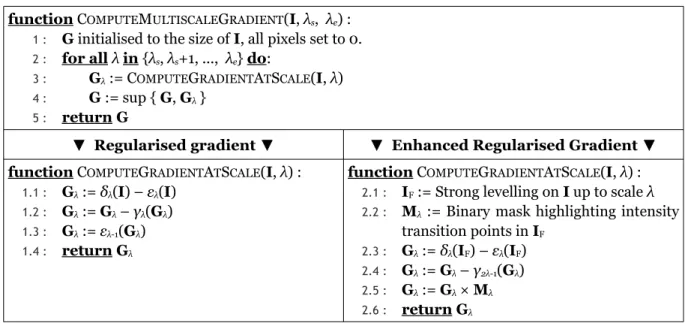
function COMPUTEMULTISCALEGRADIENT(I, λs, λe) :
1 : G initialised to the size of I, all pixels set to 0. 2 : for all λ in {λs, λs+1, ..., λe} do:
3 : Gλ := COMPUTEGRADIENTATSCALE(I, λ)
4 : G := sup { G, Gλ }
5 : return G
▼ Regularised gradient ▼ ▼ Enhanced Regularised Gradient ▼ function COMPUTEGRADIENTATSCALE(I, λ) :
1.1 : Gλ := δλ(I) – ελ(I)
1.2 : Gλ := Gλ – γλ(Gλ)
1.3 : Gλ := ελ-1(Gλ)
1.4 : return Gλ
function COMPUTEGRADIENTATSCALE(I, λ) : 2.1 : IF := Strong levelling on I up to scale λ
2.2 : Mλ := Binary mask highlighting intensity
transition points in IF
2.3 : Gλ := δλ(IF) – ελ(IF)
2.4 : Gλ := Gλ – γ2λ-1(Gλ)
2.5 : Gλ := Gλ × Mλ
2.6 : return Gλ
Table 1. Algorithms for computing the regularised gradient and the proposed enhanced gradient
(a) – Input image Original size: 1920x1080 pixels
(b) –Morphological gradient (inverted) of thickness λ=2
(c) – Regularised gradient (inverted and normalised) between scales λs=2 and λe=10
(d) – Enhanced regularised gradient (inverted) between scales λs=2 and λe=10 Figure 1. Comparison of different morphological gradients on a colour image
Computing the transition points in step 2.2
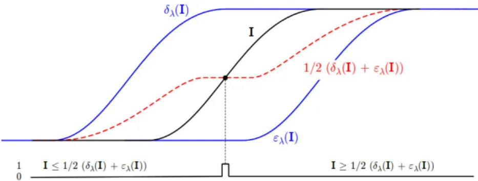
Figure 2 illustrates a smooth change of intensity along a scan-line of image I, of which the actual intensity variation may be captured using a thick gradient of size λ. The transition point corresponds to the intersection of I with the morphological average ½(δλ(I) + ελ(I)) when I is not flat. In practice
however, the equality between the input image and its morphological average is rarely verified.
It is necessary to separate the pixels of the input image I into three groups: those above, under or equal to the morphological average. Then, one performs a dilation on I, re-classifies the pixels into the three aforementioned groups and searches for those having a different classification. We consider that I has been “crossed” when a pixel changes from an “under” state to an “above” state. We mark this pixel as a transition point as illustrated in figure 3. Symmetrically, we repeat the same process after performing an erosion on I and take the union of the detections.
Figure 2. Illustrating the relationship between the brightness function and its thick morphological average
Red discs denote pixels having a value under the morphological
aver-age, purple above and white equal.
Following a dilation on input I, red discs denote pixels having a value under the morphological average,
purple above and white equal.
State transitions which yield transition points
Results and Discussion
Figure 1 compares three morphological gradients obtained from a colour image which is subject to noise and blurriness. In order to take account of the colour information, we compute the supremum of the gradients for each considered channel. Instead of using the standard red, green and blue channels, we exploit channels which are representative of the perceived brightness [Kalloniatis, 2014] and the image saturation [Demarty, 1998] .
Qualitatively, the enhanced regularised gradient clearly highlights the contours of the train, as well as its wheels, its windows and the railway. One can also better distinguish the legs of the character standing in the middle of the scene. The same goes for the radiator and the electrical plug lying in the background. Finally our gradient is the only one among the three which captures well the strong intensity transition between the penguin's leg and the stomach or the foot.
The filtering in step 2.1 clearly contributes to the output of a de-noised gradient for λs>1. It is possible
to envisage higher values of λs if one is interested in removing contours which originate from textured
objects.
Conclusion
We have proposed a revision of the morphological regularised gradient. In its enhanced version, the regularised gradient reflects the perceived contrast between the objects composing a scene. The core of the multi-scale algorithm is identical for both gradients. The principal changes consist of filtering the input image before computing the thick gradients and replacing the erosion by a detection of brightness transitions for the gradient thinning step. Both the filtering and the binary mask computation are scale-dependant. The results attest to the visual appeal of the enhanced gradient which paves the way for the processing and hierarchical segmentations of difficult images.
Acknowledgements
This work has been performed in the project PANORAMA, co-funded by grants from Belgium, Italy, France, the Netherlands, and the United Kingdom, and the ENIAC Joint Undertaking.
References
Beucher, S., Bilodeau, M., & Yu, X. (1990, April). Road segmentation by watershed algorithms. In
PROMETHEUS Workshop, Sophia Antipolis, France.
Demarty, C. H., & Beucher, S. (1998). Color segmentation algorithm using an HLS transformation.
Computational Imaging and Vision, 12, 231-238.
Kalloniatis, M., & Luu, C. (2014). Light and dark adaptation. Webvision: The organization of the
ret-ina and visual system.
Meyer, F. (2006). Levelings: theory and practice. In Handbook of Mathematical Models in Computer
Vision (pp. 63-78). Springer US.
Rivest, J. F., Soille, P., & Beucher, S. (1992, April). Morphological gradients. In SPIE/IS&T 1992
Sym-posium on Electronic Imaging: Science and Technology (pp. 139-150). International Society for