HAL Id: hal-00735686
https://hal.archives-ouvertes.fr/hal-00735686
Submitted on 26 Sep 2012HAL is a multi-disciplinary open access
archive for the deposit and dissemination of sci-entific research documents, whether they are pub-lished or not. The documents may come from teaching and research institutions in France or abroad, or from public or private research centers.
L’archive ouverte pluridisciplinaire HAL, est destinée au dépôt et à la diffusion de documents scientifiques de niveau recherche, publiés ou non, émanant des établissements d’enseignement et de recherche français ou étrangers, des laboratoires publics ou privés.
Video Segmentation and Structuring for Indexing
Applications
Ruxandra Tapu, Titus Zaharia
To cite this version:
Ruxandra Tapu, Titus Zaharia. Video Segmentation and Structuring for Indexing Applications. Inter-national Journal of Multimedia Data Engineering and Management (IJMDEM), 2012, 2 (4), pp.38-58. �10.4018/jmdem.2011100103,ISSN:1947-8534,�. �hal-00735686�
Video Segmentation and Structuring for
Indexing Applications
Ruxandra Tapu and Titus Zaharia
Institut Télécom / Télécom SudParis, ARTEMIS Department, UMR CNRS 8145 MAP5, Evry, France
ABSTRACT
This paper introduces a complete framework for temporal video segmentation. First, a computationally efficient shot extraction method is introduced, which adopts the normalized graph partition approach, enriched with a non-linear, multiresolution filtering of the similarity vectors involved. The shot boundary detection technique proposed yields high precision (90%) and recall (95%) rates, for all types of transitions, both abrupt and gradual. Next, for each
detected shot we construct a static storyboard, by introducing a leap keyframe extraction method. The video abstraction algorithm is 23% faster than existing, state of the art techniques, for
similar performances. Finally, we propose a shot grouping strategy that iteratively clusters visually similar shots, under a set of temporal constraints. Two different types of visual features are here exploited: HSV color histograms and interest points. In both cases, the precision and recall rates present average performances of 86%.
Keywords: temporal video segmentation, video indexing, shot boundary detection; key-frame extraction, video abstraction, temporal constraints; scene extraction.
INTRODUCTION
Recent advances in the field of image/video acquisition and storing devices have determined an spectacular increase of the amount of audio-visual content transmitted, exchanged and shared over the Internet. In the past years, the only method of searching information in multimedia databases was based on textual annotation, which consists of associating a set of keywords to each individual item. Such a procedure requires a huge amount of human interaction and is intractable in the case of large multimedia databases. Today, existing video repositories (e.g. Youtube, Google Videos, DailyMotion...) include millions of items. Thus, attempting to manually annotate such huge databases is a daunting job, not only in terms of money and time, but also with respect to the quality of annotation.
When specifically considering the issue of video indexing and retrieval applications, because of the large amount of information typically included in a video document, a first phase that needs to be performed is to structure the video into its constitutive elements: chapters, scenes, shots and keyframes This paper specifically tackles the issue of video structuring and proposes a complete and automatic segmentation methodology.
Fig. 1 presents the proposed analysis framework. The main contributions proposed in this paper concern: an enhanced shot boundary detection method, a fast static storyboard technique and a new scene/chapter detection approach.
The rest of this paper is organized as follows. After a brief recall of some basic theoretical aspects regarding the graph partition model exploited, we introduce the proposed shot detection algorithm. Then, we describe the keyframe selection procedure. The following section introduces a novel scene/chapter extraction algorithm based on temporal distances and merging strategies. The experimental results obtained are then presented and discussed in details. Finally, we conclude the paper and open some perspectives of future work.
Figure 1. [The proposed framework for high level video segmentation].
SHOT BOUNDARY DETECTION Related Work
The first methods introduced in the literature were based on pixels color variation between successive frames (Zhang et al., 1993), (Lienhart et al., 1997). Such algorithms offer the advantage of simplicity but present serious limitations. Thus, in the presence of large moving objects or in the case of camera motion, a significant number of pixels change their intensity values, leading to false alarms. In addition, such methods are highly sensitive to noise that may be introduced during the acquisition process.
Among the simplest, most effective and common used methods, the color histogram comparison and its numerous variations assume that frames from the same shot have similar histograms (Yuan et al., 2007), (Gargi et al., 2000). Histogram-based methods are more robust to noise and motion than pixel-based approaches due to the spatial invariance properties. However, they also present some strong limitations. First of all, let us mention the sensitivity to abrupt changes in light intensity: two images taken in the same place but with different lightening conditions will be described by distinct histograms. Furthermore, a color histogram does not take into account the spatial information of an image, so two identical histograms could actually correspond to two visual completely different images, but with similar colors and appearance probability (Matsumoto et al., 2006).
Let us also cite the methods based on edges/contours (Zabih et al., 1995). Such methods are useful in removing false alarms caused by abrupt illumination change, since they are less
sensitive to light intensity variation then color histogram (Yuan et al., 2007). However, their related detection performances are inferior to the histogram-based approaches.
Algorithms using motion features (Porter et al., 2000) or developed in the compressed domain (Fernando et al., 2001) propose an interesting alternative solution to pixel and histogram-based methods. Notably, such approaches are fairly robust with respect to camera and object motion. In addition, in this case, the detection is performed only on a partial decoded video stream therefore the computation time is reduced. However, such methods lead to inferior precision rates when compared to other methods because of incoherencies in the motion vector field. The compromise solution consists in decompressing the data up to a certain level of detail (Truong et al., 2007).
In the following section, we propose an improved shot boundary detection algorithm, based on the graph partition (GP) model firstly introduced in (Yuan et al., 2007) and considered as state of the art technique for both types of transitions: abrupt (cuts) and gradual (e.g. fades and wipes).
Graph Partition Model
The graph partition model was firstly introduced in (Hendrickson et al., 2000). The technique can be applied for video temporal segmentation by considering the input image sequence as an undirected weighted graph. In this context, we denote with G a set (V, E) where V represents the set of vertices, V = {v1,v2,…,vn}, and E V × V denote a set of pair-wise relationships, called
edges. An edge ei,j = {vi, vj}is established between two adjacent nodes.
A shot boundary detection process relaying on a graph partition system represents each video frame as a node in the hierarchical structure, connected with the other vertexes by edges (eij).
The weight (wij) of an edge (eij), expresses the similarity between the corresponding nodes (vi
and vj.). In our work, we have adopted, as visual similarity measure the chi-square distance
between color histograms in the HSV color space (equation 1):
𝑤𝑤𝑖𝑖,𝑗𝑗 = ∑ �𝐻𝐻𝑘𝑘 𝑖𝑖−𝐻𝐻 𝑘𝑘𝑗𝑗� 2 𝐻𝐻𝑘𝑘𝑖𝑖+𝐻𝐻𝑘𝑘𝑗𝑗 𝑘𝑘 × 𝑒𝑒|𝑖𝑖−𝑗𝑗| , (1)
where H i denotes the HSV color histogram associate to frame i. The exponential term in equation (1) takes into account the temporal distance between frames: if two frames are located at an important temporal distance it is highly improbable to belong to the same shot.
The video is segmented using a sliding window that selects a constant number of N frames, centered on the current frame n. The window size should be large enough to capture usual transitions. In practice, such transitions are most often greater than 10–15 frames. Thus in our work, we have considered a value of N = 25 frames.
For each position of the sliding window, the system computes a sub-graph Gn, and its
associated similarity matrix that stores all the chi-square distances between the frames
considered for analysis at the current moment. Let Vn = {vn1, vn2,..., vnN} denote the vertices of
graph Gn at frame n. For each integer k € {1,...,N-1}, a partition of the graph Gn into two sets
(𝐴𝐴𝑛𝑛𝑘𝑘 = 𝑣𝑣𝑛𝑛1, … , 𝑣𝑣𝑛𝑛𝑘𝑘), (𝐵𝐵𝑛𝑛𝑘𝑘 = 𝑣𝑣𝑛𝑛𝑘𝑘+1, … , 𝑣𝑣𝑛𝑛𝑁𝑁) is defined.
To each partition, the following objective function is associated with:
𝑀𝑀𝑀𝑀𝑀𝑀𝑀𝑀(𝐴𝐴𝑛𝑛𝑘𝑘, 𝐵𝐵𝑛𝑛𝑘𝑘) =𝑀𝑀𝑀𝑀𝑀𝑀(𝐴𝐴𝑛𝑛 𝑘𝑘, 𝐵𝐵 𝑛𝑛𝑘𝑘) 𝑎𝑎𝑎𝑎𝑎𝑎𝑎𝑎𝑀𝑀(𝐴𝐴𝑛𝑛𝑘𝑘) + 𝑀𝑀𝑀𝑀𝑀𝑀(𝐴𝐴𝑛𝑛𝑘𝑘, 𝐵𝐵𝑛𝑛𝑘𝑘) 𝑎𝑎𝑎𝑎𝑎𝑎𝑎𝑎𝑀𝑀�𝐵𝐵𝑛𝑛𝑘𝑘� , (2) ⊂
where cut and assoc respectively denote the measures of cut (i.e. dissimilarity between the two elements of the partition) and association (i.e. homogeneity of each element of the partition) and are defined as described in (3) and (4):
𝑎𝑎𝑎𝑎𝑎𝑎𝑎𝑎𝑀𝑀(𝐴𝐴𝑘𝑘𝑛𝑛) = � 𝑤𝑤𝑖𝑖,𝑗𝑗 𝑖𝑖,𝑗𝑗∈𝐴𝐴𝑛𝑛𝑘𝑘 ; 𝑎𝑎𝑎𝑎𝑎𝑎𝑎𝑎𝑀𝑀(𝐵𝐵𝑛𝑛𝑘𝑘) = � 𝑤𝑤𝑖𝑖,𝑗𝑗 𝑖𝑖,𝑗𝑗∈𝐵𝐵𝑛𝑛𝑘𝑘 , (3) 𝑀𝑀𝑀𝑀𝑀𝑀(𝐴𝐴𝑛𝑛𝑘𝑘, 𝐵𝐵𝑛𝑛𝑘𝑘) = � 𝑤𝑤𝑖𝑖,𝑗𝑗 , 𝑖𝑖∈𝐴𝐴𝑛𝑛𝑘𝑘,𝑗𝑗 ∈𝐵𝐵 𝑛𝑛𝑘𝑘 (4) The objective is to determine an optimal value for the k parameter that maximizes the
𝑀𝑀𝑀𝑀𝑀𝑀𝑀𝑀(𝐴𝐴𝑛𝑛𝑘𝑘, 𝐵𝐵𝑛𝑛𝑘𝑘) function defined in equation (2). This optimization requires to maximize the cut
function, while simultaneously minimizing both association values involved in equation 2. The optimal value, determined for each image n of the video flow, is stored in a dissimilarity vector
v = (v(n)) constructed as follows:
𝑣𝑣(𝑛𝑛) = 𝑘𝑘∈{1,…,𝑁𝑁−1}max {𝑀𝑀𝑀𝑀𝑀𝑀𝑀𝑀(𝐴𝐴𝑘𝑘𝑛𝑛, 𝐵𝐵𝑛𝑛𝑘𝑘)} , (5)
Fig.2 illustrates the dissimilarity vector obtained for different values N of the temporal analysis window.
Figure 2. [Local minimum vector variation with different window sizes (a. 10 frames, b. 15 frame, c. 25 frames and d. 35 frames) ].
A straightforward manner to identify a shot boundary is determine the peaks of the dissimilarity vector v that are higher than a considered threshold Tshot
However, in practice the selection of the threshold parameter Tshot is highly difficult due
mostly to various visual content variation caused by camera and large object movement, or by changes in the lightening conditions. An inadequate threshold may thus lead to both false alarms and missed detections. For these reasons, in contrast with (Yuan et al., 2007) and (Hendrickson
et al., 2000), we propose to perform the analysis within the scale space of the derivatives of the
local minimum vector v, as described in the next section.
Scale Space Filtering
The discrete derivative v’(n) of the dissimilarity vector v(n), can be defined in the discrete space based on the first order finite difference as:
v’(n) = v(n) – v(n–1), (6) Based on this simple relation we can construct a set of cumulative sums {𝑣𝑣𝑘𝑘′(𝑛𝑛)}𝑘𝑘=1𝑁𝑁 on the
derivative signal up the sliding window size (N) based on the following equation:
𝑣𝑣𝑘𝑘′(𝑛𝑛) = ∑𝑘𝑘𝑝𝑝=0𝑣𝑣′(𝑛𝑛 − 𝑝𝑝), (7)
The resulted signals v’k(n) represent low-pass filtered versions of the derivative signal v’(n),
with increasingly larger kernels, and constitute our scale space analysis. After summing all the above equations, within a window of analysis, v’k(n) can be simply expressed as:
𝑣𝑣𝑘𝑘′(𝑛𝑛) = 𝑣𝑣(𝑛𝑛) − 𝑣𝑣(𝑛𝑛 − 𝑘𝑘); (8)
Fig.3 presents the dissimilarity signal obtained at different scales. As it can be observed, smoother and smoother versions of the original signal are produced, which can be useful to remove undesired variations caused by camera/large object motions.
Figure 3. [The set of scale space derivatives obtained].
The peaks which are persistent at multiple resolutions correspond to large variations in the feature vector and are used to detect the shot transitions.
The selection of the identified peaks is performed based on a different non-linear filtering operation that is applied at each scale of analysis, defined as described by the following equation.
𝑑𝑑(𝑛𝑛) = max
𝑘𝑘 {|𝑣𝑣𝑘𝑘
′(𝑛𝑛)| ∙ ℎ(𝑘𝑘)} = max
𝑘𝑘 {|𝑣𝑣(𝑛𝑛) − 𝑣𝑣(𝑛𝑛 − 𝑘𝑘)| ∙ ℎ(𝑘𝑘)}, (9)
ℎ(𝑘𝑘) = �𝑒𝑒 −𝑘𝑘, 𝑘𝑘 ∈ �0,𝑁𝑁 − 1 2 � 𝑒𝑒𝑁𝑁−1−𝑘𝑘, 𝑘𝑘 ∈ �𝑁𝑁 + 1 2 , 𝑁𝑁� , (10)
The shot boundaries detection process is applied directly on the d(n) signal. The weighting mechanism adopted, given by the h(n) function, privileges derivative signals located at the extremities of the scale space analysis (Fig. 4). In this way, solely peaks that are persistent through all scales are retained and considered as transitions.
Figure 4. [False alarms due to flash lights, large object/camera motion are avoided when using the scale-space filtering approach].
The second step of the proposed shot boundary detection system is focused on reducing the computational complexity of the proposed shot detector. In this context, a two pass analysis technique is introduced.
Two Pass Analysis Approach
The principle consists of successively applying two different analysis stages.
In a first stage, the objective is to determine video segments that can be reliable classified as belonging to the same shot. In order to identify such segments, a simple and fast chi-square comparison on HSV color histogram between each two successive frames is performed. In this step we can identify also abrupt transition that characterized by large discontinuity values (Fig.5).
Figure 5. [Classification of video in certain/uncertain segments]. Video stream
Concerning the detection process we have considered two thresholds. The first one, denoted by Tg1 has to be selected high enough to avoid the false positives. The second threshold Tg2 is
used in order to determine uncertain time intervals. If the dissimilarity values are above the second threshold (D(It, It–1)>Tg2), and also inferior to Tg1 a more detailed analysis is required and
the method passes to the second step. All frames presenting lower similarity values, (i.e. smaller than Tg2) are classified as belonging to the same shot.
In a second stage, for the remaining uncertain intervals (for which a reliable classification could not be made only by performing a simple chi-square distance analysis), we apply the graph partition method with scale space filtering previously described.
In this manner, the total number of images that require a detailed analysis is considerably reduced. The second phase helps us differentiate between actual gradual transition and local variations in the feature vector caused by object or camera motion.
For each detected shot, we aim at determining a set of keyframes that can represent in a significant manner the associated content.
KEYFRAME EXTRACTION Related Work
One of the first attempts to automate the keyframe extraction process was to consisted in selecting as a keyframe the first, the middle or the last frame (or even a random one) of each detected shot (Hanjalic et al., 1999). However, while being sufficient for stationary shots, a single frame does not provide an acceptable representation of the visual content in the case of dynamic sequences that exhibit large camera/object motion. Therefore, it is necessary to consider more sophisticated approaches (Fu et al., 2009).
The challenge in automatic keyframe extraction is given by the necessity of adapting the selected keyframes to the underlying content, while maintaining, as much as possible, the original message and removing all the redundant information. In (Zhang et al., 1999), the first keyframe is set as the first frame in a shot appearing after a shot boundary. A set of additional keyframes is determined based on the variation in color/motion appearance with respect to this first frame. However, the approach does not take into account of the case of gradual transitions, where the first keyframe is not an optimal choice and might negatively influence the whole keyframe selection process.
A clustering algorithm (Girgensohn et al., 1999) is the natural solution to solve the problems described above. The limitations here are related to the threshold parameters that need to be specified and which have a strong impact on both the cluster density and on the related computational cost.
A mosaic-based approach can generate, in an intuitive manner, a panoramic image of all informational content existed in a video stream. The summarization procedure in this case is based on the assumption that there is only one dominant motion among all the others various object motions found in the sequence (Aner et al., 2002). Mosaic-based representations of shot / scene include more information and are visually richer than regular keyframe approaches. However, creating mosaics is possible solely for videos with specific camera motion, such as pan, zoom or tilling.
In the case of movies with complex camera effects such as a succession of background/foreground changes, mosaic-based representations return less satisfactory results due
to physical location inconsistency. Furthermore, mosaics can blur certain foreground objects and thus present a degraded image quality.
In our case, we have developed a keyframe representation system that extracts a variable number of images from each detected shot, adaptively with the visual content variation.
Leap-Extraction Method
For each detected shot, a first keyframe is defined as the frame located N frames away after the detected transition (i.e., the beginning of the shot). Let us recall that N denotes the window size used for the shot boundary detection method. In this way, we make sure that the first selected keyframe does not belong to a gradual effect.
In the second phase, we developed a leap-extraction method that analyzes only the frames spaced by multiple integers of window size N and not the entire set of frames as in the case of the reference techniques introduced in (Zhang et al., 1999), (Rasheed et al., 2005). Then, in order to select a new keyframe the current image is compared (i.e. chi-square distance of HSV color histograms) with all the keyframes already extracted. If the visual dissimilarity is above a pre-established threshold the new image is marked as representative and is added to the set of keyframes (Fig. 6).
Figure 6. [Keyframe selection based on leap-extraction technique].
The leap keyframe extraction method takes advantage of the shot boundary detection system that computes the graph partition within a sliding window of analysis. In this way, the proposed method ensures that all the relevant information will be taken into account. As it can be observed, the number of keyframes necessary to describe the informational content of a shot is not a priori fixed, but automatically adapted to the dynamics of the content.
An additional post-processing step is introduced. The goal is to eliminate, from the selected set of keyframes, all the blank images that might appear (Chasanis et al., 2008). Such images can appear due to gradual transitions developed over a large number of frames or to false alarms. They are often encountered in real life videos and it is necerssaryto remove them in order to ensure the quality of the detected summary (Li et al., 2010). . The adopted technique exploits a contour-based approach. Here, the total number of edges detected in a keyframe is analyzed in order to determine such blank images.
A final contribution concerns the shot clustering within scenes.
SCENE SEGMENTATION
A scene is defined in the Webster’s dictionary as follows: “a subdivision of an act or a play in which the setting is fixed, the time is continuous and the action is developed in one place”. Such a definition involves some purely semantic elements, related to the unity of time, place and action that are difficult to determine automatically when performing solely vision-based analysis. This makes the scene detection process a highly difficult issue.
In addition, in some circumstances and from a purely visual point of view, such constraints may not hold, as in the case of scenes with large camera/object motion.
For all these reasons, elaborating methods for pertinent and automatic scene identification is still an open issue of research. Let us first analyze how these aspects are treated in the rich literature dedicated to this subject.
Related Work
In (Rasheed et al., 2005), authors transform the detection problem into a graph partition task. Each shot is represented as a node being connected with the others through edges based on the visual similarity and the temporal proximity between the shots. A new measure, so-called shot
goodness (SG), is here introduced. The SG measure quantifies the degree of representativeness
of each shot, based on its temporal length, visual activity and action content.
In (Hanjalic et al., 1999), the detection process relays on the concept of logical story units (LSU) and inter-shot dissimilarity measure. The LSU definition is based on the temporal
consistency of the visual content assuming that similar elements (e.g. people, faces, locations …) appear and some of them even repeat. So, a LSU gathers a set of successive shots, connected by overlapping links. The shots regrouped in a same LSU present similarity values superior to an adaptive threshold set by the user.
Different approaches (Ariki et al., 2003) propose to use both audio features and low level visual descriptors in order to detect scenes separately based on both characteristics. In this case, two types of boundaries are detected and used to make a final decision. A scene is defined based on audio sequences as a succession of shots in which a similar audio pattern occurs (e.g. dialog between two characters, cheering crowd …) (Truong et al., 2007). The audio segments are divided in: background and foreground. Only the foreground segments are analyzed in order to make a decision because the background soundtrack is assumed not to carry any information that may be relevant to the film story.
In (Ngo et al., 2002), color and motion information are integrated in order to take a decision. The motion analysis is based on the tensor determination in order to establish the slices (set of 2D images in a x, y t space) with horizontal and vertical positions.
A mosaic-based approach is introduced in (Aner et al., 2002). The value of each pixel in the mosaic is defined as the median value of pixels corresponding to all the frames mapped in the mosaic image. The scene boundaries are determined after segmenting the mosaic in small regions and analyzing the similarities between such adjacent regions.
More recent techniques (Chasanis et al., 2009), (Zhu et al., 2009) introduce in the analysis process useful concepts such as temporal constraints and visual similarity.
However, the existing approaches show strong limitations and present limited precision and recall rates (77% to 82%).
In order to deal with the complexity of the scene detection task this paper proposes a novel approach, based on a hierarchical clustering algorithm with and temporal constraints.
Scene Detection Method
The algorithm takes as input the set of keyframes detected for the whole set of video shots as described in the previously. A clustering process is then applied. The principle consists of iteratively grouping shots encountered in a temporal sliding analysis window that satisfy simultaneously a set of similarity constraints.
The size of the sliding window (denoted by dist) is adaptively determined, based on the input video stream dynamics and is proportional to the average number of frames per shot. The parameter dist can be computed as:
𝑑𝑑𝑖𝑖𝑎𝑎𝑀𝑀 = 𝛼𝛼 ∙𝑇𝑇𝑎𝑎𝑀𝑀𝑎𝑎𝑇𝑇 𝑛𝑛𝑀𝑀𝑛𝑛𝑛𝑛𝑒𝑒𝑛𝑛 𝑎𝑎𝑜𝑜 𝑜𝑜𝑛𝑛𝑎𝑎𝑛𝑛𝑒𝑒𝑎𝑎𝑇𝑇𝑎𝑎𝑀𝑀𝑎𝑎𝑇𝑇 𝑛𝑛𝑀𝑀𝑛𝑛𝑛𝑛𝑒𝑒𝑛𝑛 𝑎𝑎𝑜𝑜 𝑎𝑎ℎ𝑎𝑎𝑀𝑀𝑎𝑎 , (11) where α denotes a user-defined parameter. We consider further that a scene is completely
described by its constituent shots:
𝑆𝑆𝑇𝑇: 𝑎𝑎(𝑆𝑆𝑇𝑇) = �𝑎𝑎𝑇𝑇,𝑝𝑝�𝑝𝑝=1𝑁𝑁𝑇𝑇 → ��𝑜𝑜𝑇𝑇,𝑝𝑝,𝑖𝑖�𝑖𝑖=1𝑛𝑛𝑇𝑇,𝑝𝑝�𝑝𝑝=1 𝑁𝑁𝑇𝑇
, (12) where Sl denotes the lth video scene, Nl the number of shots included in scene Sl, sl,p the pth shot
in scene Sl, and fl,p,i the ith keyframe of shot sl,p. containing nl,p keyframes.
The proposed scene change detection algorithm based on shot clustering consists of the following steps:
Step 1: Initialization – The technique starts by assigning the first shot of the input video stream to the first scene S1. Scene counter l is set to 1.
Step 2: Shot to scene comparison – The next shot being analyzed (i.e. a shot that is not assigned to any already created scene) is considered as the current shot and denoted by scrt. the
technique determines The subset Ω of all anterior scenes located at a temporal distance inferior to the parameter dist with respect to the current shot scrt is then determined. The visual similarity
between each scene Sk in Ω and the shot scrt is computed as described by the following relation:
∀𝑆𝑆𝑘𝑘 ∈ Ω, 𝑆𝑆𝑀𝑀𝑒𝑒𝑛𝑛𝑒𝑒𝑆𝑆ℎ𝑎𝑎𝑀𝑀𝑆𝑆𝑖𝑖𝑛𝑛(𝑎𝑎𝑀𝑀𝑛𝑛𝑀𝑀, 𝑆𝑆𝑘𝑘) =𝑛𝑛 𝑛𝑛𝑛𝑛𝑎𝑎𝑀𝑀𝑀𝑀 ℎ𝑒𝑒𝑑𝑑
𝑘𝑘,𝑝𝑝∙ 𝑁𝑁𝑘𝑘 ∙ 𝑛𝑛𝑀𝑀𝑛𝑛𝑀𝑀 , (13)
where ncrt is the number of keyframes of the considered shot and nmatched represents the number
of matched keyframes of the scene Sk. A keyframe from scene Sk is considered to be matched
with a keyframe from shot scrt if a given visual similarity measure between the two keyframes is
superior to a threshold Tgroup. Let us note that a keyframe from the scene Sk can be matched with
multiple frames from the current shot.
Two different types of visual similarity measures have been considered:
(1) the total number of common interest points established based on a SIFT descriptor (Lowe, 2004) and matched with the help of a KD-tree technique (Vedaldi et al., 2010), and (2) the chi-square distance between HSV color histograms.
The current shot scrt is identified to be similar to a scene Sk if the following condition is
satisfied:
𝑆𝑆𝑀𝑀𝑒𝑒𝑛𝑛𝑒𝑒𝑆𝑆ℎ𝑎𝑎𝑀𝑀𝑆𝑆𝑖𝑖𝑛𝑛(𝑆𝑆𝑘𝑘, 𝑎𝑎𝑀𝑀𝑛𝑛𝑀𝑀) ≥ 0.5, (14)
The relation 13 expresses that at least half of the keyframes belonging to the current shot scrt
need to be similar with the scene’s Sk keyframes.
In this case, the current shot scrt is clustered in the scene Sk. In the same time, all the shots
between the current shot and the scene Sk will also be attached to scene Sk and marked as
neutralized. Then all scenes containing neutralized shots are automatically removed, in the sense
that they are attached to the scene Sk. The list of detected scenes is consequently updated.
The neutralization process allows us to identify the most representative shots for a current scene (Fig. 7), which are the remaining non-neutralized shots. In this way, the influence of outlier shots which might correspond to some punctual digressions from the main action in the considered scene is minimized.
Figure 7. [Neutralizing shots (marked with red) based on visual similarity].
If the condition described in equation (13) is not satisfied, go to step 3.
Step 3: Shot by shot comparison – Here, we determine the set of highly similar shots (i.e., with a similarity value at least two times bigger than the grouping threshold Tgroup ). Here, for the
current shot (scrt) we compute its visual similarity with respect to all shots of all scenes included
in the sub-set Ω determined at step 2. If the shot scrt is found as being highly similar with a scene
in Ω, then it is merged with the corresponding scene, together with all the intermediate shots. If
scrt is found highly similar to multiple scenes, than the scene which is the most far away from the
considered shot is retained.
Both the current shot and all its highly similar matches are unmarked and for the following clustering process will contribute as normal, non-neutralized shots (Fig. 8).
This step ensures that shots that are highly similar with other shots in a previous scene are be grouped into this scene. In this way, the number of false alarms (i.e., false scene transitions) is considerably reduced.
Step 4: Creation of a new scene – If none of the conditions introduced in steps 2 and 3 are satisfied, then a new scene, containing the current shot (scrt), is created.
Step 5: Refinement –The scenes containing only one shot are automatically deleted and their shot is attached to the adjacent scenes based on the highest similarity value. In the case of the first scene, the corresponding shot will be grouped to the following one by default.
Figure 8. [Unmarking shots based on high similarity values (red – neutralized shots; green – non-neutralized shots)].
The grouping threshold Tgroup is established adaptively with respect to the input video stream
visual content variation, for each visual similarity measure considered (i.e. HSV color histogram or interest points). Thus, Tgroup is defined as as the average chi-square distance / number of
interest points between the current keyframe and all anterior keyframes located at a temporal distance smaller then dist.
EXPERIMENTAL RESULTS Shot Boundary Detection
In order to evaluate our shot boundary detection algorithm, we have considered a sub-set of videos from the “TRECVID 2001 and 2002 campaigns”, which are available on Internet
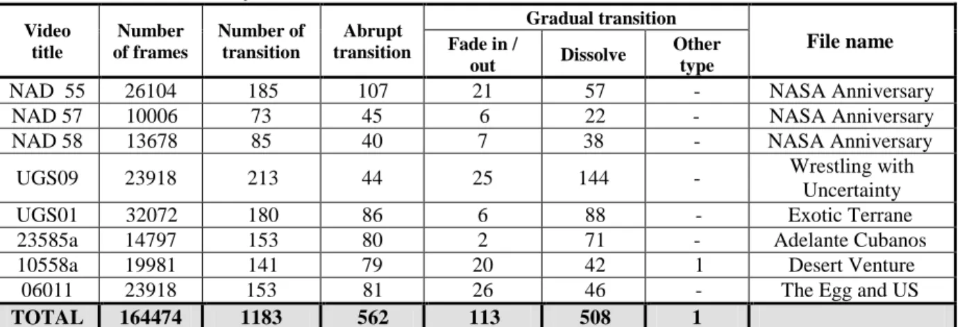
(www.archive.org and www.open-video.org). The videos are mostly documentaries that vary in style and date of production, while including multiple types of both camera/object motion (Table 1).
Table 1. Movie database features.
Video title Number of frames Number of transition Abrupt transition Gradual transition File name Fade in / out Dissolve Other type
NAD 55 26104 185 107 21 57 - NASA Anniversary
NAD 57 10006 73 45 6 22 - NASA Anniversary
NAD 58 13678 85 40 7 38 - NASA Anniversary
UGS09 23918 213 44 25 144 - Wrestling with
Uncertainty
UGS01 32072 180 86 6 88 - Exotic Terrane
23585a 14797 153 80 2 71 - Adelante Cubanos
10558a 19981 141 79 20 42 1 Desert Venture
06011 23918 153 81 26 46 - The Egg and US
TOTAL 164474 1183 562 113 508 1
As evaluation metrics, we have considered the traditional Recall (R) and Precision (P) measures, defined as follows:
Here, D is the number of the detected shot boundaries, MD is the number of missed detections, and FA the number of false alarms. Ideally, both recall and precision should be equal to 100%, which correspond to the case where all existing shot boundaries are correctly detected, without any false alarm.
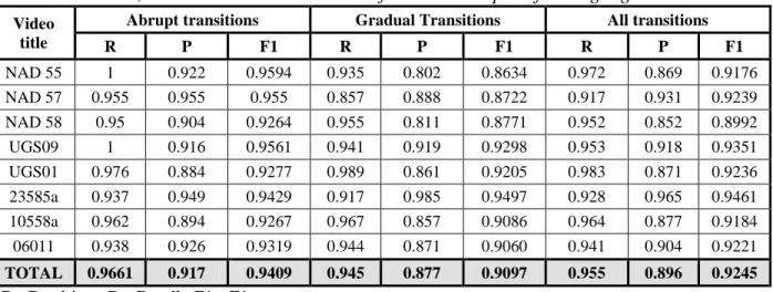
Table 2 presents the precision, recall and F1 rates obtained for the reference graph partition shot boundary detection method proposed by Yuan et al. (Yuan et al., 2007), while Table 3 summarizes the detection performances of our proposed scale-space filtering approach.
Table 2. Precision, recall and F1 rates obtained for the Yuan et al. algorithms
Video title
Abrupt transitions Gradual Transitions All transitions
R P F1 R P F1 R P F1 NAD 55 0.9626 0.824 0.8879 0.8717 0.7391 0.7999 0.9243 0.788 0.8507 NAD 57 0.8666 0.8666 0.8666 0.7857 0.8148 0.7999 0.8472 0.8472 0.8472 NAD 58 0.95 0.8444 0.8940 0.7777 0.6603 0.7142 0.8588 0.7448 0.7977 UGS09 0.9727 0.8431 0.9032 0.8106 0.7740 0.7918 0.8866 0.7894 0.8351 UGS01 0.9069 0.8472 0.8760 0.8404 0.7523 0.7939 0.8722 0.8579 0.8649 23585a 0.75 0.923 0.8275 0.7945 0.9666 0.8721 0.7712 0.944 0.8488 10558a 0.8607 0.8717 0.8661 0.7741 0.923 0.8420 0.8226 0.8923 0.8560 06011 0.9135 0.9024 0.9079 0.8333 0.7228 0.7741 0.8756 0.8121 0.8426 TOTAL 0.8950 0.8627 0.8785 0.8164 0.7812 0.7984 0.8610 0.8198 0.8398
P – Precision ; R – Recall ; F1 – F1 norm
Table 3. Precision, recall and F1 rates obtained for the scale-space filtering algorithm
Video title
Abrupt transitions Gradual Transitions All transitions
R P F1 R P F1 R P F1 NAD 55 1 0.922 0.9594 0.935 0.802 0.8634 0.972 0.869 0.9176 NAD 57 0.955 0.955 0.955 0.857 0.888 0.8722 0.917 0.931 0.9239 NAD 58 0.95 0.904 0.9264 0.955 0.811 0.8771 0.952 0.852 0.8992 UGS09 1 0.916 0.9561 0.941 0.919 0.9298 0.953 0.918 0.9351 UGS01 0.976 0.884 0.9277 0.989 0.861 0.9205 0.983 0.871 0.9236 23585a 0.937 0.949 0.9429 0.917 0.985 0.9497 0.928 0.965 0.9461 10558a 0.962 0.894 0.9267 0.967 0.857 0.9086 0.964 0.877 0.9184 06011 0.938 0.926 0.9319 0.944 0.871 0.9060 0.941 0.904 0.9221 TOTAL 0.9661 0.917 0.9409 0.945 0.877 0.9097 0.955 0.896 0.9245
P – Precision ; R – Recall ; F1 – F1 norm
The results presented clearly demonstrate the superiority of our approach, for both types of abrupt (Fig. 9) and gradual transitions (Fig. 10). The global gains in recall and precision rates are of 9.8% and 7.4%, respectively (Fig. 11).
Moreover, when considering the case of gradual transitions, the improvements are even more significant. In this case, the recall and precision rates are respectively of 94,1% and 88,3% (with respect to R = 81.5% and P = 79% for the reference method (Yuan et al., 2007)). This shows that
the scale space filtering approach makes it possible to eliminate the errors caused by camera/object motion.
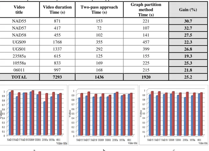
Concerning the computational aspects, Table 4 synthesizes the results obtained, in computational time, with the two-pass approach (cf. Section II) compared to the initial scale-space filtering method.
Here, for the chi-square, frame-to-frame HSV color histogram comparison we considered for the first threshold (Tg1) a value of 0.9 to detect abrupt transition, while the seconf (Tg2) has been
set to 0.35.
Such values ensure the same overall performance of the shot boundary detection as the multi-resolution graph partition method applied on the entire video stream. A smaller value for the Tg1
will determine an increase in the number of false alarms while a higher values for Tg2 will
increase the number of missed detected transitions.
Table 4. Computation time for GP and two-pass approach
Video title Video duration Time (s) Two-pass approach Time (s) Graph partition method Time (s) Gain (%) NAD55 871 153 221 30.7 NAD57 417 72 107 32.7 NAD58 455 102 141 27.5 UGS09 1768 355 457 22.3 UGS01 1337 292 399 26.8 23585a 615 125 155 19.3 10558a 833 169 225 25.3 06011 997 168 215 21.8 TOTAL 7293 1436 1920 25.2
Figure 9. [Recall (a.), Precision (b.) and F1 norm (c.) rates when detecting abrupt transitions for: a. Yuan et al. algorithm (blue), b. The novel scale space derivative technique (red)].
Figure 10. [Recall (a.), Precision (b.) and F1 norm (c.) rates when detecting gradual transitions for: a. Yuan et al. algorithm (blue), b. The novel scale space derivative technique (red)].
Figure 11. [Recall (a.), Precision (b.) and F1 norm (c.) rates when detecting all types of transitions for: a. Yuan et al. algorithm (blue), b. The proposed technique (red)].
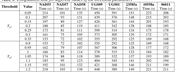
Table 5 presents the computational times for different values for the threshold parameter. The experimental results were obtained for Tg1 constant and Tg2 variable and vice-versa.
Table 5. Computation time for different values of the threshold parameters
Threshold Value NAD55
Time (s) NAD57 Time (s) NAD58 Time (s) UGS09 Time (s) UGS01 Time (s) 23585a Time (s) 10558a Time (s) 06011 Time (s) Tg1 0.05 214 101 135 450 391 151 223 208 0.1 207 93 131 439 376 148 215 203 0.15 197 89 127 426 361 144 201 193 0.2 188 85 119 411 342 138 188 185 0.25 173 81 111 399 319 134 175 178 0.3 161 75 105 373 305 129 172 171 0.35 153 72 102 355 292 125 169 168 Tg2 0.9 153 72 102 355 292 125 169 168 0.95 162 79 107 367 306 128 177 172 1 166 83 114 378 315 133 184 182 1.05 174 88 118 389 332 137 193 189 1.1 183 95 123 404 345 141 202 194 1.15 192 101 132 421 368 146 211 199 1.2 218 103 138 448 389 149 221 211 a. b. c. a. b. c.
Results presented in Table 5 lead to the following conclusion. With the increase of the threshold Tg1 and respectively with the reduction of the Tg2 the computational time is decreasing. Let us
also mention that the values parameter Tg1 shouldbe inferior to 0,35 and the value of Tg2 greater
than 0.9 in order to maintain the same performances in terms of detection efficiency.
Leap Keyframe Extraction
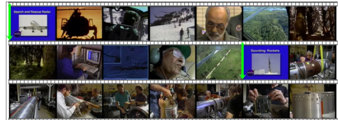
For each detected shot we applied the leap extraction method described. Fig. 12 presents a set of keyframes detected from of a complex shot which exhibits important visual content variation (because of very large camera motion). In this case, the proposed algorithm automatically determines a set of 6 keyframes.
Figure 12. [Shot boundary detection and keyframe extraction].
Table 6 presents the computational time1
Video title
necessary to extract keyframes for two methods: (1) the proposed leap-extraction strategy, and (2) the state-of-the-art method (Zhang et al.,
1999), (Rasheed et al., 2005) based on direct comparison of all adjacent frames inside a shot. Let us note that the obtained key-frames are quite equivalent in both cases.
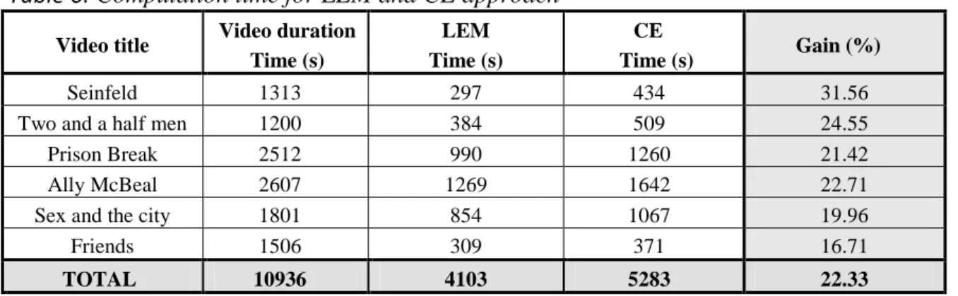
Table 6. Computation time for LEM and CE approach
Video duration Time (s) LEM Time (s) CE Time (s) Gain (%) Seinfeld 1313 297 434 31.56
Two and a half men 1200 384 509 24.55
Prison Break 2512 990 1260 21.42
Ally McBeal 2607 1269 1642 22.71
Sex and the city 1801 854 1067 19.96
Friends 1506 309 371 16.71
TOTAL 10936 4103 5283 22.33
LEM- Leap Extraction Method, CE – Classical Extraction
The results presented in Table 6 demonstrate that the proposed approach makes it possible to significantly reduce the computational complexity for the keyframe detection algorithms, for
equivalent performances. Thus, the leap keyframe extraction method leads to a gain of 22% in computational time when compared to the state of the art method.
Scene/DVD Chapter Extraction
The validation of our scene extraction method has been performed on a corpus of 6 sitcoms and 6 Hollywood movies (Tables 6 and 7) also used for evaluation purposes in the state of the art algorithms presented in (Rasheed et al., 2005), (Chasanis et al., 2009), (Zhu et al., 2009).
Fig. 13 illustrates some examples of scene boundary detection, obtained with the HSV-based approach.
Figure 13. [Detected scenes].
We can observe that in this case the two scenes of the movie have been correctly identified. In order to establish an objective evaluation, for the considered database, a ground truth has been established by human observers. Table7 summarizes the scene detection results obtained with both visual similarity measures adopted (i.e. SIFT descriptors and HSV color histograms).
Table 7. Evaluation of the scene extraction: precision, recall and F1 rates
Video name
Ground truth scenes
SIFT descriptor HSV color histogram
D FA MD R (%) P (%) F1 (%) D FA MD R (%) P (%) F1 (%) Sienfeld 24 19 1 5 95.00 79.16 86.36 20 0 4 100 83.33 90.88 Two and a half men 21 18 0 3 100 81.81 90.00 17 2 4 89.47 80.95 85.01 Prison Break 39 31 3 8 91.17 79.48 84.93 33 0 6 100 84.61 91.66 Ally McBeal 32 28 11 4 71.79 87.50 78.87 24 4 8 84.00 75.00 79.24 Sex and the city 20 17 0 3 100 85.00 91.89 15 1 5 93.75 75.00 83.33 Friends 17 17 7 0 70.83 100 82.92 17 7 0 70.83 100 82.92 5th Element 63 55 24 8 69.62 87.30 77.46 54 10 9 83.05 84.48 83.76 Ace -Ventura 36 34 11 2 75.55 94.44 83.95 29 2 7 92.85 78.78 85.24 Lethal Weapon 4 67 63 39 4 61.76 94.02 74.55 64 25 3 71.97 95.52 82.05 Terminator 2 66 61 11 5 84.72 92.42 88.41 60 7 6 89.55 90.90 90.22 The Mask 44 40 5 4 88.88 90.91 89.88 38 7 6 84.44 86.36 85.39 Home Alone 2 68 56 6 12 90.32 82.35 86.15 57 5 11 90.90 81.96 86.20 TOTAL 497 439 118 58 88.32 78.81 83.29 428 70 69 86.11 85.94 86.02
As it can be observed, the detection efficiency is comparable in both cases. The α parameter has been set here to a value of 7.
The average precision and recall rates are the following: • R=88% and P=78%, for the SIFT-based approach, and • R=86% and P=85%, for the HSV histogram approach.
These results demonstrate the superiority of the proposed scene detection method with respect to existing state of the art techniques (Rasheed et al., 2005), (Chasanis et al., 2009), (Zhu et al., 2009), which provide precision/recall rates between 82% and 77%.
We also analyzed the impact of the different temporal constraints lengths on the scene detection performances. Thus, Fig. 14 presents the precision, recall and F1 scores obtained for various values of the α parameter.
As it can be noticed, a value between 5 and 10 returns quite similar results in terms of the overall efficiency.
Figure 14. [Precision, recall and F1 scores obtained for different α values].
Let us also observe that increasing the α parameter lead to lower recall rates. That means that for higher values of the α parameter, different scenes are grouped within a same one. In the same time, the number of false alarms (i.e. false scene breaks) is reduced.
This observation led us to investigate the utility of our approach for a slightly different application, related to DVD chapter detection. For the considered Hollywood videos, the DVD chapters were identified by movie producers and correspond to access points in the considered video. The DVD chapters are highly semantic video units with low level of detail containing a scene ore multiple scenes that are grouped together based on a purely semantic meaning.
The value of the α parameter has been here set to 10.
The average recall (R) and precision (P) rates obtained in this case (Fig.15) are the following: • R=93% and P=62%, for the SIFT-based approach, and
• R=68% and P=87%, for the HSV histogram approach.
Such a result is quite competitive with the state of the art techniques introduced in (Rasheed et
al., 2005), (Chasanis et al., 2009), (Zhu et al., 2009) which yield precision/recall rates varying
between 65% and 72%.
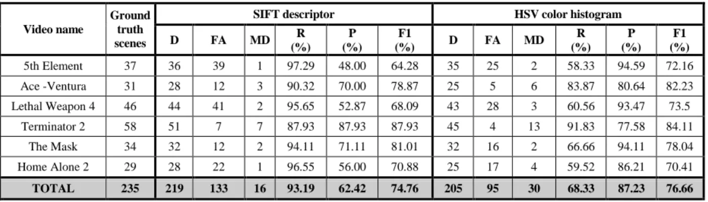
The obtained chapter detection results, with precision, recall and F1 rates are further detailed in Table 8.
Figure 15. [Recall, Precision and F1 norm rates when extracting DVD chapter using: a. HSV color histogram, b. Interest points extracted based on SIFT descriptor].
Table 8. Evaluation of the DVD chapter extraction: precision, recall and F1 rates
Video name
Ground truth scenes
SIFT descriptor HSV color histogram
D FA MD R (%) P (%) F1 (%) D FA MD R (%) P (%) F1 (%) 5th Element 37 36 39 1 97.29 48.00 64.28 35 25 2 58.33 94.59 72.16 Ace -Ventura 31 28 12 3 90.32 70.00 78.87 25 5 6 83.87 80.64 82.23 Lethal Weapon 4 46 44 41 2 95.65 52.87 68.09 43 28 3 60.56 93.47 73.5 Terminator 2 58 51 7 7 87.93 87.93 87.93 45 4 13 91.83 77.58 84.11 The Mask 34 32 12 2 94.11 71.11 81.01 32 16 2 66.66 94.11 78.04 Home Alone 2 29 28 22 1 96.55 56.00 70.88 25 17 4 59.52 86.21 70.41 TOTAL 235 219 133 16 93.19 62.42 74.76 205 95 30 68.33 87.23 76.66
D – Detected ; FA – False Alarms ; MD – Missed Detected; P – Precision ; R – Recall ; F1 – F1 norm
The analysis of the obtained results leads to the following conclusions.
The keyframe similarity based on HSV color histogram is much faster than the SIFT
extraction process. In addition, it can be successfully used when feature detection and matching becomes difficult due to the complete change of the background, important variation of the point of view, or complex development in the scene’s action.
The matching technique based on interest points is better suited for scenes that have
undergone some great changes but where some persistent, perennial features (such as objects of interest) are available for extraction and matching. In addition, the technique is robust to abrupt changes in the intensity values introduced by noise or changes in the illumination condition.
It would be interesting, in our future work, to investigate how the two methods can be efficiently combined in order to increase the detection performances.
CONCLUSION AND PERSPECTIVES
In this paper, we have proposed a novel methodological framework for temporal video
structuring and segmentation, which includes shot boundary detection, keyframe extraction and scene identification methods.
The main contributions proposed involve: (1) an enhanced shot boundary detection method based on multi-resolution non-linear filtering and with low computational complexity; (2) a leap keyframe extraction strategy that generates adaptively static storyboards; (3) a novel shot
clustering technique that creates semantically relevant scenes, by exploiting a set of temporal constraints, a new concept of neutralized/ non-neutralized shots as well as an adaptive
thresholding mechanism.
The shot boundary detection methods is highly efficient in terms of precision and recall rates (with gains up to 9.8% and 7.4%, respectively in the case all transitions with respect to the reference state of the art method), while reducing with 25% the associated computational time.
Concerning the shot grouping into scenes, we have validated our technique by using two different types of visual features: HSV color histograms and interest points with SIFT descriptors. In both cases, the experimental evaluation performed validates the proposed approach, with a F1 performance measure of about 86%.
Finally, we have shown that for larger temporal analysis windows, the proposed algorithm can also be used to detect DVD chapters. The experimental results demonstrate the robustness of our approach, which provides an average F1 score of 76%, regardless the movie’s type or gender.
Our perspectives of future work will concern the integration of our method within a more general framework of video indexing and retrieval applications, including object detection and recognition methodologies. Finally, we intend to integrate within our approach motion cues that can be useful for both reliable shot/scene/keyframe detection and event identification.
REFERENCES
Aner, A., & Kender, J. R. (2002): Video summaries through mosaic-based shot and scene clustering, in Proc. European Conf. Computer Vision, 388–402.
Ariki Y., Kumano M., & Tsukada K. (2003). Highlight scene extraction in real time from baseball live video. Proceeding on ACM International Workshop on Multimedia Information
Retrieval, 209–214.
Chasanis V., Likas A., & Galatsanos N. P. (2008). Video rushes summarization using spectral clustering and sequence alignment. In TRECVID BBC Rushes Summarization Workshop
(TVS’08), ACM International Conference on Multimedia, 75–79.
Chasanis, V., Kalogeratos, A., & Likas, A. (2009). Movie Segmentation into Scenes and Chapters Using Locally Weighted Bag of Visual Words, Proceeding of the ACM International
Conference on Image and Video Retrieval.
Fernando, W.A.C, Canagarajah, C.N., & Bull, D.R. (2001). Scene change detection algorithms for content-based video indexing and retrieval, IEE Electronics and Communication Engineering
Journal, 117–126.
Fu, X., & Zeng, J. (2009). An Improved Histogram Based Image Sequence Retrieval Method,
Proceedings of the International Symposium on Intelligent Information Systems and Applications (IISA’09), 015-018.
Furini M., & Ghini V. (2006). “An audio–video summarization scheme based on audio and video analysis, Proceedings of the IEEE Consumer Communications and Networking Conference (CCNC ’06), vol. 2, 1209–1213.
Gargi, U., Kasturi R., & Strayer, S. (2000). Performance characterization of video shot-change detection methods, IEEE Trans. Circuits and Systems for Video Technology, Vol.CSVT-10, No.1 1-13.
Girgensohn, A., & Boreczky, J. (1999). Time-Constrained Keyframe Selection Technique, in
IEEE Multimedia Systems, IEEE Computer Society, Vol. 1, 756- 761.
Hanjalic A, Lagendijk RL, & Biemond J (1999). Automated high-level movie segmentation for advanced video-retrieval systems, IEEE Circuits Syst Video Technol 9, 580–588.
Hanjalic, A., & Zhang, H. J. (1999). An integrated scheme for automated video abstraction based on unsupervised cluster-validity analysis, IEEE Transactions on Circuits and Systems for Video
Technology, vol. 9, no. 8.
Hendrickson, B., & Kolda, T. G. (2000). Graph partitioning models for parallel computing,
Parallel Computing Journal, Nr. 26, 1519-1534.
Li Y., & Merialdo B. (2010), “VERT: a method for automatic evaluation of video summaries”,
ACM Multimedia; pp. 851-854.
Lienhart, R., Pfeiffer, S., & Effelsberg, W. (1997). Video Abstracting, Communications of the
ACM , 1 -12.
Lowe, D. (2004). Distinctive image features from scale-invariant keypoints, International
Journal of Computer Vision, 1-28.
Matsumoto K., Naito M., Hoashi K., & F.Sugaya (2006). “SVM-Based Shot Boundary Detection with a Novel Feature,” In Proc. IEEE Int. Conf. Multimedia and Expo, 1837–1840.
Ngo C.W., & Zhang H.J. (2002). Motion-based video representation for scene change detection.
Internation Journal in Computer Vision 50(2), 127–142.
Porter, S.V., Mirmehdi, M., & Thomas, B.T. (2000). Video cut detection using frequency domain correlation, 15th International Conference on Pattern Recognition, 413–416.
Rasheed, Z., Sheikh, Y., & Shah, M. (2005). On the use of computable features for film classification, IEEE Trans. Circuits Syst. Video Technol., vol. 15, no. 1, 52–64.
Truong B., Venkatesh S. (2007). Video abstraction: A systematic review and classification, ACM
Transactions on Multimedia Computing, Communications, and Applications (TOMCCAP), v.3
Yuan, J., Wang H., Xiao L., Zheng W., Li, J., Lin, F.,& Zhang, B. (2007). A formal study of shot boundary detection, IEEE Trans. Circuits Systems Video Tech., vol. 17, 168–186.
Zabih, R., Miller, J., & Mai, K. (1995). A feature-based algorithm for detecting and classifying scene breaks, Proc. ACM Multimedia 95, 189–200.
Zhang, H., Wu, J., Zhong, D., & Smoliar, S. W. (1999). An integrated system for content-based video retrieval and browsing, Pattern Recognition., vol. 30, no. 4, 643–658.
Zhang, H.J., Kankanhalli, A., & Smoliar, S.W. (1993). Automatic partitioning of full-motion video, Multimedia Systems no. 1, 10–28.
Zhu, S., & Liu, Y. (2009). Video scene segmentation and semantic representation using a novel scheme, Multimedia Tools and Applications, vol. 42, no. 2, 183-205.
Vedaldi,A., & Fulkerson, B. (2010). VLFeat: An open and portable library of computer vision algorithm, http://www.vlfeat.org.