Quantitative Stereovision in a Scanning Electron Microscope

HAL Id: hal-01644885

https://hal.archives-ouvertes.fr/hal-01644885

Submitted on 23 Feb 2018

HAL is a multi-disciplinary open access

archive for the deposit and dissemination of

sci-entific research documents, whether they are

pub-lished or not. The documents may come from

teaching and research institutions in France or

abroad, or from public or private research centers.

L’archive ouverte pluridisciplinaire HAL, est

destinée au dépôt et à la diffusion de documents

scientifiques de niveau recherche, publiés ou non,

émanant des établissements d’enseignement et de

recherche français ou étrangers, des laboratoires

publics ou privés.

Quantitative Stereovision in a Scanning Electron

Microscope

T. Zhu, M. A. Sutton, N. Li, Jean-José Orteu, Nicolas Cornille, Xiaojian Li,

A. P. Reynolds

To cite this version:

T. Zhu, M. A. Sutton, N. Li, Jean-José Orteu, Nicolas Cornille, et al.. Quantitative Stereovision in a

Scanning Electron Microscope. Experimental Mechanics, Society for Experimental Mechanics, 2011,

51 (1), pp.97-109. �10.1007/s11340-010-9378-7�. �hal-01644885�

Quantitative Stereovision in a Scanning Electron Microscope

X. Li&A.P. Reynolds

Abstract Accurate, 3D full field measurements at the micron level are of interest in a wide range of applications, including both facilitation of mechanical experiments at reduced length scales and accurate profiling of specimen surfaces. Scanning electron microscope systems (SEMs) are a natural platform for acquiring high magnification images for stereo reconstruction. In this work, an integrated methodology for accurate three dimensional metric reconstruction and deformation measurements using single column SEM imaging systems is described. In these studies, the specimen stage is rotated in order to obtain stereo views of the specimen as it undergoes mechanical or thermal loading. Simulations and preliminary experimental studies at 300× demonstrate that (a) spatially varying image distortions can be removed from images using a non parametric distortion model, (b) the system can be reliably calibrated using distortion corrected images of a planar object and grid at various orientations and (c) specimen rotation variability during the measurement

phase can be controlled so that baseline strain errors are within the range of ±150 µε. Benchmark rigid body motion experiments using calibrated SEM views demonstrate that all components of strain in the reconstructed object have a mean value around O(10 4_{) and a random spatial distribution with} standard deviation≈300 micro strain.

Keywords Scanning electron microscope (SEM) . Stereo vision . Digital image correlation (DIC) . Strain measurement . Accurate 3D topography and 3D displacement measurements

Introduction

Deformation and profile measurements continue to be impor tant issues for mechanical testing at micro/nano scales [1 3]. At these scales, Scanning Electron Microscope (SEM) images have been combined with modern non contacting measure ment methods such as Digital Image Correlation (DIC) to make accurate 2D measurements on nominally planar speci mens [4 6]. As the experiments at smaller scales become increasingly sophisticated and material behavior in the vicinity of 3D micro scale features is required, the need for three dimensional shape and full field strain and deformation measurements has expanded. One discipline where such measurements are of interest is biomedical engineering [7 11]. The ability to obtain accurate 3D measurements using single column SEM images presents several challenges, including (a) three dimensional metric reconstruction using single column SEM images, (b) correction of image distortions, (c) development of an effective procedure for acquiring images from multiple views, (d) calibration of the stereo image views and (e) appropriate theoretical description for stereo reconstruction over a wide range of applications. Three dimensional profiling using one imag T. Zhu

:

:

:

:

A.P. Reynolds

Department of Mechanical Engineering, University of South Carolina,

Columbia, SC 29205, USA e mail: [email protected] J. J. Orteu (SEM member)

Université de Toulouse, INSA, UPS, Mines Albi, ISAE, ICA (Institut Clément Ader),

Campus Jarlard, F 81013 Albi, France

e mail: jean jose.orteu@mines albi.fr N. Cornille

G2Métric,

40 Chemin Cazalbarbier, 31140 Launaguet, France

ing device and multiple images acquired from different orientations is a classic problem in photogrammetry for which there are multiple applications using SEM images [12 27]. In general, such applications have three shortcomings when considering extension for deformation measurements. First, since a typical photogrammetric reconstruction is scale free [28], the approach is inappro priate for deformation or profile measurements. Secondly, the accuracy of the reconstruction is significantly degraded by disregarding the distortion associated with SEM images. For example, when using DIC to extract profile measure ments, Lockwood et al. [27] obtained results assuming a reduced form for the imaging equations and negligible distortions. In fact, it was only with the publication of a series of recent articles [4, 12, 29, 30] that the effects of spatially varying and temporarily varying distortions in SEM images were identified as being important, and then quantified at magnifications varying from 200× to 20,000× [4,29,30]. Finally, the operations necessary to obtain and analyze several SEM images to profile a specimen are tedious, especially if multiple profiles are needed over time. In this paper, a method for obtaining three dimensional deformations using a sequence of SEM images acquired during out of plane specimen rotation is described. Vision system parameters for each view are separated for effective calibration through independent procedures. The non parametric spatial distortion model [31] is employed to remove spatial distortions from each image view using in plane motions of a planar target. All SEM images used for calibration and deformation measurements are converted into distortion free SEM images by removing the spatial distortions. To demonstrate the methodology, a benchmark experiment is performed to reconstruct the three dimensional motions and deformations for a planar specimen undergoing three separate 3D rigid

body motions. Residual strain fields computed from the reconstructed motions are presented which demonstrate the accuracy of the SEM stereovision measurement system.

Imaging in an SEM

The imaging process in an SEM system is fundamentally different from an optical system. Whereas an optical imaging system employs lenses to collect and focus light waves, a modern SEM system scans an e beam across the specimen surface and collects back scattered (or secondary) electrons using a fixed detector to construct an image.

A simplified schematic of the imaging process for an SEM is shown in Fig.1. As the electron beam scans across the surface, backscattered electrons (BSEs) ejected from the interaction volume are collected by a stationary BSE detector (generally centrally located near the e beam) for each “point” in the scan area. Since the electron scan and the BSE location do not change as the specimen is translated out of plane, the resulting image of the translated specimen will be for shortened, as shown in Fig.1for a specific pair of feature points.

Since optical images will also be for shortened when the specimen is translated out of plane (or tilted), an established optical imaging model (pinhole model) has been shown to be appropriate to describe the perspective effect for our relatively low magnification SEM studies. A mathematical description for the pinhole model given in equation (1) [31 33] that relates two dimensional coordinates in an SEM image to the coordinates of the corresponding 3D world coordinates of a feature point on the specimen can be written;

r ! m ¼ A½ $3%3! R t½ $3%4! M ð1Þ where m xs ys 1 8 > < > : 9 > = > ;;M Xw Yw Zw 1 8 > > > < > > > : 9 > > > = > > > ; ; A½ $_3%3 fx fs Cx 0 fy Cy 0 0 1 2 6 4 3 7 5; t tx ty tz 8 > < > : 9 > = > ;;R cos g sin g 0 sin g cos g 0 0 0 1 2 6 4 3 7 5 cos b 0 sin b 0 1 0 sin b 0 cos b 2 6 4 3 7 5 1 0 0 0 cos a sin a 0 sin a cos a 2 6 4 3 7 5

where xf s ysgT represents two dimensional sensor coor

dinates of a point in a digital SEM image in pixel units; ρ is a factor in metric units;1 _X

w Yw Zw

f gT represents

the three dimensional world coordinates of point. The

matrix [A] contains the intrinsic camera parameters including fx, fy, fsand the image center location, (Cx, Cy) in pixels that describe the camera to image projection transformation. The matrix R is the rotation matrix relating the world and camera coordinate system orienta tion. The form shown in equation (1) is associated with Euler angles α, β and γ [34]. The vector t defines the world to camera system translation vector with compo nents tx, tyand tz,in metric units.

1_{This factor is defined to convert the pinhole perspective model into a} homogeneous form [31] with constant matrices (for example, matrix [A]). Inspection of equation (1) shows that ρ is determined by the last equation and is a function of R, M and t, varying with each world point of interest.

Single Camera Stereovision: Equivalency with Dual Camera

Quantitative 3D reconstruction can be performed using a single “camera,” even when there is no a priori knowledge of camera parameters. Using established photogrammetric principles [28], a general procedure for such situations is to acquire a sequence of images of an object using different “camera” orientations and positions. In such cases, it is well known that three dimensional reconstruction using images from several unknown views [28] can be performed up to an unknown scale factor [28]. In such cases, it is common practice to place an object with known metric distance in each view, providing sufficient information to define the scale factor.

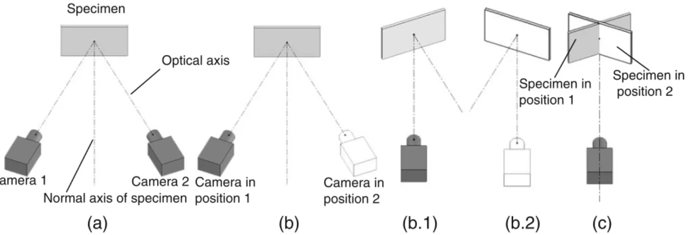
In a similar manner, photogrammetric approaches can be employed to develop an equivalent stereo vision methodol ogy for use with standard, single column SEM imaging systems. Figure 2 demonstrates the relationship between multi camera stereovision systems and multi view, single camera stereovision systems. In fact, the three stereovision systems shown in 2(a), 2(b) and 2(c) are equivalent. The mathematical model in equation (1) for the standard system in 2(a) can be applied to the other two systems directly, with differences in interpretation of the extrinsic parameters defined in the following section. By imposing constraints that require the two viewing angles (specimen rotations2in 2 (c)) to be repeatable, the SEM can be considered as a Tilting Specimen Stereovision (TSSV) system. As will be demon strated in the following sections, the operational constraint imposed by this requirement can be controlled experimen tally so that the resulting strain errors are relatively small (more detail is provided in “Reconstruction Error Due to

Rotation Angle Variations”). For the TSSV system, there is only one imaging device involved, so that only one set of intrinsic parameters is required for both views.

Prior to presenting the formulation for the TSSV system, it must be emphasized that common terms in optical imaging (“view,” “camera,” “orientation of views” and “translation between views”) are still used throughout this article, though the terms have different meaning in SEM imaging. For example, “views” correspond to different specimen tilts in SEM imaging; “camera” corresponds to the combination of EBSD detector and digital image converter in the SEM; “orientation of views” corresponds to different specimen tilts, not different sensor array orientations; “translation between views” corresponds to an artificial motion (the true translation is actually near zero) required by the pinhole model to construct convergent specimen views.

Tilting Specimen Stereovision System

Consider two views of an object point, Mi, as shown schematically in Fig. 3. Letting the coordinate system for the first view be the world system, one can write equation (1) for each view as follows:

r1i! m1i¼ A½ $ ! I 0½ $ ! Mi r_{2i! m}2i¼ A½ $ ! R t½ $ ! Mi ( ð2Þ where m1i¼ xf s1i ys1i 1g T_{; x} s1i, ys1i represent the

coordinates of the ith_{point in the first SEM view in pixels;} m2i¼ xf s2i ys2i 1g

T_{; x}

s2i, ys2irepresents the coordinates

of the ith_{point in the second SEM view in pixels; ρ} 1iand ρ2i are two factors corresponding to each view; Mi represents the world coordinates of the ith _{point in metric} units [see equation (1)]. As noted previously, in this description the world coordinate system is set to coincide with the coordinate system of the first view as shown in Fig.3. Thus, [A] is the intrinsic parameter matrix for both the first and second views, where I is a 3×3 identity matrix and 0 is the 3×1 zero translation vector. The matrix [R t] contains the extrinsic parameters including [R] the rotation

2_{Specimen rotations about an axis that is nominally orthogonal to the} e beam in an SEM are typically known as “specimen tilts” using a “tilt stage” in the microscopy community. Since Euler angles also are known as “pan”, “tilt” and “swing”, the authors opted to use the terminology “specimen rotation” or “out of plane rotation” instead of “specimen tilt” to define the reorientation of the specimen to obtain stereo views. Specimen in position 1 Specimen in position 2 E-gun Feature point Image of specimen in position 1 Image of specimen in position 2 6 pixels 4 pixels Fig. 1 Perspective effect in

matrix relating the first and second views and [t] the translation vector from the first view to the second view. System Calibration and Distortion Removal

The calibration procedure for standard stereovision systems yields optimal parameters by fitting the stereovision model in equation (2) to the corresponding measurement locations in both views simultaneously; details are given in a series of recent publications [31,32,35]. Though the approach is appealing due to previous successes, direct adoption for TSSV system calibration will introduce significant error because the specimen rotation angle (α) normally considered constant during calibration will vary slightly during the experiment, making the calibration algorithm unstable. For the above reason, the investigators adopted a sequential approach for system calibration, as described in the following paragraphs.

Distortion correction

It has been shown in recent articles [4,29,30] that optimal accuracy in SEM based image measurements using a pinhole model requires that SEM image distortions be considered and methods developed to quantify these distortions. According to Sutton et al. [4], there are two types of distortion embedded in an SEM image temporally varying (drift) and spatially varying (spatial) distortion. When SEM images of a conducting specimen are taken at low magnification (less than 1,000X), temporally varying distor tion oftentimes can be neglected. For the experiment presented in “Experimental Validation in SEM,” drift distortion is neglected, though straight forward application of previous drift correction methods is appropriate for use in the SEM stereo imaging at higher magnification.

Due to the complexity of spatially varying distortion in SEM images (see Fig.4), non parametric distortion correc tion approaches [35] are employed. The procedure described in previous work employs images of a planar object subjected to a series of in plane translations to identify the distortion field and remove it from subsequent images. For a single column SEM, a distortion correction function is determined by in plane translation of a planar specimen that is nominally orthogonal to the e beam central axis. Since the distortion field is assumed to be a function of only the pixel location in the image, the distortion corrections are applied to all images obtained from any orientation.

Intrinsic parameters calibration

The calibration target (grid with dots at known spacing) shown in the top part of Fig.5is placed in the SEM and imaged as it undergoes several rotations and translations. The grid images after distortion correction are used in the calibration process.

.

.

Fig. 3 Stereo model parameters. The angle between the two views is the sum of the individual rotations, +/ θ, relative to the normal and is designatedα Camera 1 _{Camera in} position 2 Camera in position 1 Camera 2 Specimen Specimen in position 2

(b)

(b.1)

(b.2)

(c)

(a)

Normal axis of specimen

Fig. 2 Equivalent stereovision systems (a) Standard Stereovision (SSV, [31]) with two identical cameras imaging at positions symmetric about the specimen normal axis; (b) Moving Camera Stereovision (MCSV), position 1 and position 2 are the positions of Camera 1 and 2 in 1(a) respectively; (b.1) and (b.2) are individual representations for a camera in position 1 and 2, respectively; (c) Tilting Specimen Stereovision (TSSV), the images of the specimen in position 1 and 2 can be decoupled to give the same perspective as shown in (b.1) and (b.2)

The standard bundle adjustment approach [31,32,36] with equation (1) is used to obtain all intrinsic parameters, extrinsic orientations and grid positions for each grid orien tation and position. Only the intrinsic parameters character izing the SEM image process are retained since the extrinsic parameters are not required for future 3D reconstruction.

It is noted that the use of a planar calibration target with known dot spacing imaged at different orientations (two orientations at least) is sufficient to constrain the param eters for the vision system [31, 32]. Repeatability of the intrinsic parameter estimation process is verified by independent experiments conducted under the same imaging conditions (see Table 1).3 _{Though the image} center locations (Cx, Cy) have variations of O(102), they are still acceptable considering the large focal lengths (fx and fy≈25,000 ). Extrinsic orientation and position parameters in equation (1), which are actually part of the

reconstruction of the dots in the world coordinate system, are not included in Table1.

Extrinsic parameters calibration

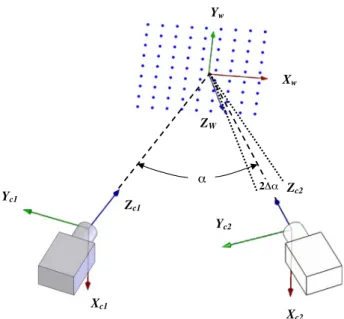
After completing the intrinsic parameter calibration process, the glass slide with the grid is moved slightly so that the dense random speckle pattern shown in Fig.5fills the field of view. Since the glass slide already is attached to a eucentric rotation stage, it is rotated out of plane by +θ and θ for use in our experimental studies and SEM images are acquired from both orientations. Figure 6 presents a schematic of the two views, with variability in the angle α=2θ clearly identified. Constraining [A] to be the same for both views, optimization of the following form with known [A] is used to determine the orientation, R and the position, t of the second view relative to the first view,

r ¼ min R t ! " ;Mi # $X n i 1 m1i( 1 r1i! A½ $ ! I 0½ $ ! Mi % &2 þ m2i( 1 r2i! A½ $ ! R t½ $ ! Mi % &2! ð3Þ

where n is the number of data points used for optimization. The optimal solution of [R t] is unique under the following 6 theoretical constraints:

i) 5 constraints from point correspondences

ii) at least 1 constraint requiring a metric distance between feature points identifiable in both views.

See AppendixAfor a brief description of the underlying theory.

Regarding the need for constraint ii), as shown in Fig.3 the vector t defines the location of the pinhole in one stereo view relative to the other pinhole. The magnitude, |t|, is also known as the baseline distance, i.e. the distance joining the two optical centers. To remove ambiguity (see AppendixA) and uniquely define |t|, the common approach is to identify at least two feature points in both views with known metric distance between them. Using the calibration parameters and the known pixel positions of the end points, an equation can be written that provides an additional constraint. By solving this equation (or several equations using optimization if multiple pairs of feature points with

x (pixels) x (pixels)

y (pixels)

Distortion (pixels) Vertical distortion field

Horizontal distortion field

y (pixels) 0.98 0.05 -0.64 -0.64 -1.57 -1.34 0.05 -0.64 -1.11 1.67 1.67

Fig. 4 Image distortion fields for Quanta 200 at 300× with imaging parameters given in “SEM Stereo Calibration”

3_{Extrinsic orientation and position parameters defined in equation (1)} and computed during the calibration process are not used for subsequent calibration procedures and hence are not included in Table1.

known metric distance are used), the vector t is uniquely defined.

Using both equation (3) and constraint ii), Table2shows the extrinsic camera parameters for Exp 1, Exp 2 and Exp 3. As noted in equation (1), α, β, γ are Euler angles and tx, ty, tzare the translations in the x , y and z directions in the rotated camera 1 coordinate system.

To obtain these values, all images of the object were distortion corrected prior to performing the optimization process.4 _{Point correspondence input into equation (3) is} obtained by feature registration algorithms such as DIC, where the number of correspondences can reach the order of 104_{. The large number of point correspondences} improves the stability of the optimization process, though at least five point correspondences are required.

Reconstruction Error Due to Rotation Angle Variations Slight variations in the total specimen rotation angle, which corresponds to the pan angleα in equation (2) (see Figs. 2 and 6), will introduce operational errors in the deformation measurements due to inaccuracies in the calibration relation ship defined for the two views and used for image reconstruction. These errors will be in addition to reconstruc tion errors introduced during subset matching employed in 3D DIC [37 39]. In the following section, relative operational rotation error (Δα) is defined by the following equation:

Δa ¼ aþ c ( ac # $ ( aþe ( ae # $ ! " ð7Þ where aþ c ( ac # $

is the calibrated total pan angle, °; and aþ

e ( ae

# $

is the experimental total pan angle, °.The relationship between Δα and strain measurement errors is

the focus of the following discussion. Numerical simulations (AppendixB) are used to investigate this relationship.

To demonstrate the effect ofΔα on strain measurement errors, the authors selected initial rotation angles that were consistent with the upper limits expected for SEM applica tions,+_{α=10° and α = 10°. The range for Δα used in the} simulations is 0.20°≤Δα≤0.20°, which spans the range of errors obtained from a series of baseline specimen rotation experiments using the SEM specimen rotation stage. No distortion is considered in this simulation.

First, two images of a 9×9 grid with 0.04 mm grid spacing are generated using the parameters from Exp 3 in Tables1and2, with the pan angle perturbed byΔα. Then, the “realized” 3D positions of the object are reconstructed using the “known” parameters (i.e., the parameters from Exp 3 in Tables1and2). The artificial displacement from the real 3D positions to the “realized” 3D positions can be computed. The artificial strains introduced by Δα are determined using a local quadratic fit to all 5×5 arrays within the 9×9 data set, averaging the resulting data to obtain a singe value for each strain component. The results for the dominant strain error, εyy, show a well defined linear relationship between the strain field bias andΔα. Fitting a straight line

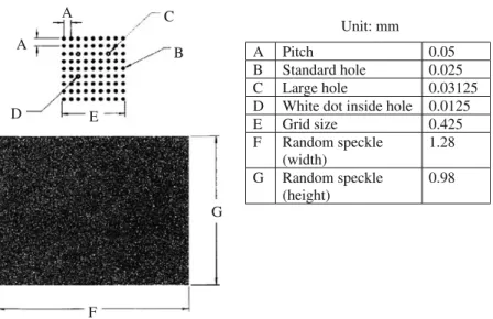
A Pitch 0.05

B Standard hole 0.025

C Large hole 0.03125

D White dot inside hole 0.0125

E Grid size 0.425 F Random speckle (width) 1.28 G Random speckle (height) 0.98 Unit: mm A A B C D E G F

Fig. 5 Grid and random pattern specimen. (Black is the etched region)

Table 1 Intrinsic parameters from three independent experiments, with spatially varying distortion correction, Magnification 300×, Working distance 10 mm Cx (Pixels) Cy (Pixels) fx (Pixels) fy (Pixels) fs (Pixels) Exp 1 350.5 195.3 24040 24080 107.9 Exp 2 35.34 245.7 25340 25370 121.5 Exp 3 410.4 129.9 25320 25340 94.62

Cx, Cy, fx, fy, fsare parameters in the intrinsic parameters matrix 4_{A slightly modified version of the commercial software Vic 3D [40]}

to the strain error vsΔα data for each strain component, we have the following form;

"xx¼ (2:38 % 10 6! Δa "yy¼ 1530 % 10 6! Δa "xy¼ (2:50 % 10 6! Δa 8 < : ð8Þ

For the case being considered, equation (8) shows that the strain bias is less than 150 µε for deformation measurements performed at a magnification of 300× whenΔα<0.10°.

Experimental Validation in SEM

To demonstrate the potential of the proposed stereo vision methodology using SEM images, a benchmark experiment was performed to reconstruct a planar object undergoing three dimensional rigid body motions. The procedure used to complete the experiments is detailed in AppendixCand includes (a) SEM spatial distortion correction, (b) SEM stereo calibration, (c) SEM experimental process and (d) image processing for three dimensional shape and motion measurements. All experiments were performed using an

FEI Quanta 200 ESEM. The eucentric goniometer stage within the FEI chamber was used to perform all rotations; operational errors were demonstrated to be less than 0.10°. Images were acquired at 300×, with the following imaging parameters: High vacuum mode; 30.0 kV working voltage; Spot size=5.0; Backscattered electron detector for all imaging; Working distance=10.0 mm; Frame time=4.73 s. Specimen Preparation

Both a 9 by 9 calibration grid and the random speckle pattern used for image correlation were manufactured by etching a glass plate coated with a 120 nm thick layer of Chrome/Chrome Oxide using a multi step optical reduction process [41] (see Fig. 5). The combination of Chrome/ Chrome Oxide and glass provides good contrast at a magnification of 300× in SEM. For higher magnifications, advanced etching processes such as FIB milling may be applied to manufacture the specimen pattern.

Distortion Removal

In this work, drift distortion is neglected since baseline imaging at 300× magnification without motion confirmed that drift was negligible over the 60 min required to complete the experiment. As noted in Appendix C, spatial distortion removal followed procedures used previously by one of the authors [35], employing a series of translated images of the specimen to extract the vector spatial distortion field. Figure 4 shows the as computed spatial distortions for both viewing directions. These distortions are removed from all SEM images. The complicated shape of the distortion field explains why normal parametric distortion model cannot be used to characterize the distortions embedded within SEM images.

SEM Stereo Calibration

The intrinsic parameters for both views and the rigid body coordinate transformations for each grid view are obtained using the distortion free SEM images of a standard grid (see Fig. 5 and Appendix C). To obtain the relative

Xw Yw ZW Yc1 Xc2 Yc2 Zc2 Xc1 Zc1 2∆α α

Fig. 6 Schematic for stereo imaging with variability in the included viewing angle. Grid rows and columns are parallel to the world coordinates, Xwand Ywrespectively, while Zwis perpendicular to the planar grid

Table 2 Extrinsic parameters from three independent experiments, with spatially varying distortion correction, Magnification 300×, Working distance 10 mm

α (°) β (°) γ (°) tx(mm) ty(mm) tz(mm)

Exp 1 20.81 0.03 0.29 0.06 8.18 1.74

Exp 2 20.75 0.25 0.34 0.15 8.62 1.83

Exp 3 20.83 0.15 0.30 0.12 9.45 2.01

Table 3 Calibration parameters for Exp 3

Intrinsic parameters Extrinsic parameters

Cx(Pixels) 410.4 α (°) 20.83 Cy(Pixels) 129.9 β (°) 0.15 fx(Pixels) 25320 γ (°) 0.3 fy(Pixels) 25340 tx(mm) 0.12 fs(Pixels) 94.62 ty(mm) 9.45 ts(mm) 2.01

orientation and position of the two views (i.e., the extrinsic parameters), distortion corrected speckle images5from both views are used with the known intrinsic parameters. The number of point correspondences used to calibrate the extrinsic parameters is ≈24,000 in this experiment. To uniquely define the baseline vector, t, for the two stereo views, internal SEM software, XDOC,6_{is used to estimate} the metric distance between two feature points. By using image correlation to locate these feature points in both stereo views, an additional equation is obtained and used in the optimization process to remove ambiguity in t. Equation (A.3) demonstrates one form of the relationship between components of t and any 3D position

Table 3 presents both the intrinsic and extrinsic parameters for the SEM stereo vision pinhole model. The angle α (which corresponds to the sum of the specimen rotation angles) is consistent with the estimated 20° specimen rotation during the experiment.

SEM Rigid Body Motion Experiments

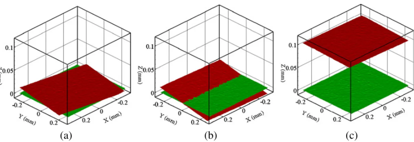
A series of rigid body motion experiments was performed to demonstrate the proposed methodology. The motions included (a) in plane rotation, (b) out of plane rotation and (c) large, out of plane translation. For each experi ment, a total of 140×140 subsets with subset size 27×27 and subset spacing of 5 pixels were compared to obtain ≈19,600 three dimensional data points. Figure 7presents the reconstructed profiles for the translated specimen (red or dark gray), with the original specimen as the reference

(green or light gray). Results show that (a) the recon structed shape of the object is not distorted by rigid body motion and (b) the measured motions are qualitatively consistent with the actual motions.

Using a least squares procedure, the measured motions for each case were computed. The actual motions of the specimen are read from the goniometer and displacement sensors on the sample manipulation stage, with reported accuracy in these results of 0.01mm. Table 4 presents a direct comparison between the measured and actual motions. As shown in Table 4, the measured results are within the error band for the motions applied to the specimen in each case.

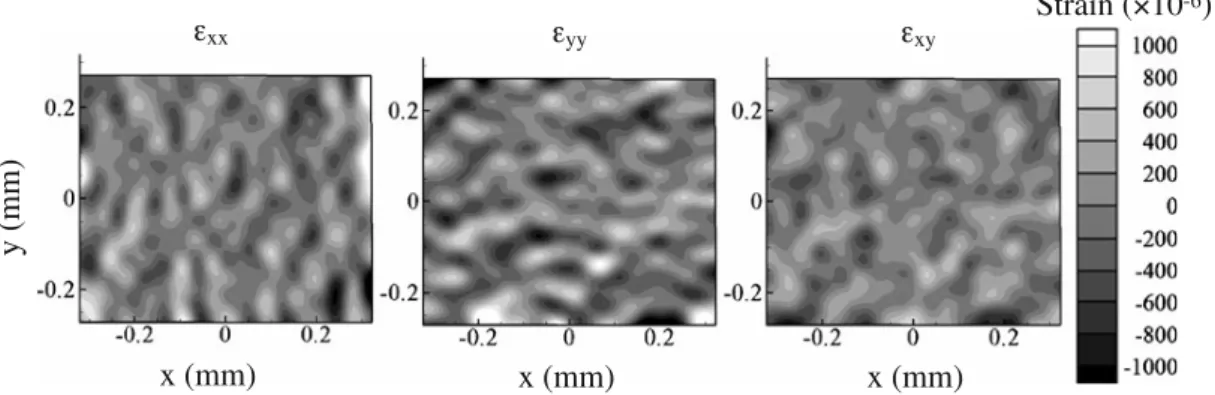
Further validation of the measurement method was performed by extracting in plane strains from the 3D measurements. Using commercial software [40], a 15×15 smoothing window and 5 pixel spacing between measure ment points, the strain distributions were computed for each case. Figure8shows the measured strain fields for out of plane rotation of 2°; similar results were obtained for 10o rotation and 0.10mm out of plane motion.

As shown in Fig.8, the measured strains are generally random in nature, confirming that the effects of spatial distortion and other imaging anomalies are properly accounted for in the measurement process. Table 5

(a)

(b)

(c)

Fig. 7 Comparison of reconstructed surface before (green, or light color) and after rigid body motion (red, or dark color) for (a) 10° in plane rotation; (b) 2° out of plane rotation; (c) 0.1 mm out of plane displacement

5_{The large number of 3D points obtained with speckle images} improved the stability and repeatability of the estimated extrinsic parameters for the two views.

6_{Software on Quanta 200 SEM manufactured by FEI Corporation}

Table 4 Measured and actual motions

Motion type Measured motiona _{Actual motion}

10° in plane rotation 10.00º±0.01º 10.0º±0.1º 2° out of plane rotation 1.92º±0.01º 2.0º±0.2º 0.1 mm out of plane

motion

0.1015±0.0003 mm 0.10±0.01 mm a_{Mean value ± 1 standard deviation}

presents quantitative data for the measured strains for all three cases.

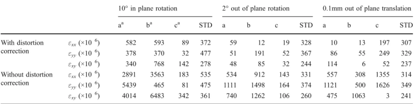
Table 6 presents the coefficients of least squares fit planes to the artificial strain data. As shown in Table6, the slopes of the artificial strains with distortion correction are much smaller than the ones without distortion correction which further confirms that the distortion correction removes bias not only in the mean value but also in the distributions. Standard deviations in Table 6are relative to the model plane instead of the mean value in Table5.

Discussion of Results

As shown in Table 5, strain data for all motions has relatively high variability due to the effects of intensity noise, scanning inaccuracy and associated SEM imaging artifacts. The largest variability occurred for in plane rotation. Since in plane rotation introduces considerable displacement within the complex image distortion field (see Fig.4), both the slight bias and the variability within the in plane rotation data are in part due to inaccuracies in the distortion correction process.

The small out of plane rotational motion results have quite small bias in all components, confirming that the stereo approach is effective in quantifying the three dimensional motion of the points when the motions fall within the depth

of field for the imaging system. The largest strain bias (e.g. deviation of mean value from zero) was observed for the out of plane motion experiment where the specimen translated beyond the calibration volume7_{and slightly defocused after} motion occurred. Even so, the results are encouraging and demonstrate that the stereo approach will remove most of the effects associated with out of plane motion, even when the image is near the edges of the focus region.

Finally, it should be noted that an important, yet quite subtle, contribution of this work is to demonstrate conclu sively that the spatial distortion correction procedure developed and validated for stationary optical imaging systems can be successfully used to identify and remove similar distortions from all SEM images, including those obtained at various specimen tilt angles. In essence, our work has shown that “spatial distortion” in an SEM image is only a function of the pixel position in the resulting image and is not altered in any way by specimen tilt or other motions.

Concluding Remarks

To ensure that the accuracy of the rotation stage is adequate for measurements, simulations can be performed to quan tify the potential strain bias as a function of Δα. Using simulation results, the required accuracy of the positioning stage can be estimated so that the appropriate stage can be selected.

For cases with higher magnification in an SEM, it is likely that drift distortions will be important and hence should be considered to optimize measurement accuracy. The method proposed by Sutton et al. [4] can be used to remove both drift distortion and spatially varying distortion in each stereo view.

7_{Calibrated volume is defined as the smallest rectangular volume that} contains all the grid and speckle points used in calibration procedure in world coordinate system.

Strain (×10

₎

x (mm)

x (mm)

x (mm)

y (mm)

ε

ε

ε

Fig. 8 Measured strain distribution after 2° out of plane rotation

Table 5 Quantitative data for strain measurements with distortion correction 10º in plane rotation 2º out of plane rotation 0.1mm out of plane translation

Mean STD Mean STD Mean STD

"xxð%10(6Þ 89 399 19 329 197 307

"yyð%10(6Þ 32 486 52 369 249 330

To calibrate the intrinsic parameters at higher magnifi cation, it is possible to manufacture and use high resolution grids by modern focused ion beam technology at both the micro scale and nano scale. Tolerance on the accuracy of the grid spacing during manufacturing can be relaxed using bundle adjustment algorithms [31,36] so that positions of the slightly offset grid points are also optimized.

For those investigators interested in metric reconstruc tions, the critical role of determining the scale constant ω must be emphasized, as the entire calibration process outlined in this work requires this constraint.

Conclusions

In this paper, the basic experimental approach for develop ment and use of a stereovision system with SEM images is presented. Using existing stereovision models, with an appropriate interpretation for both calibration and recon struction to remove scale ambiguity, single column SEM images acquired at different tilt angles can be shown to provide a robust platform for three dimensional measure ments at high magnification.

The effect of operational error introduced during specimen rotation to define two stereo views is analyzed by simulation and results are used to guide the rotation operations for the eucentric goniometer stage. Repeatability and accuracy of measurements is demonstrated through independent calibration experiments and rigid body motion experiments, with strain bias O(10 4_{) and strain variability} O(3×10 4_{) demonstrated through multiple experiments.}

Acknowledgements The technical support of Dr. Hubert Schreier and Correlated Solutions Incorporated is deeply appreciated. The financial support provided by (a) Dr. Stephen Smith through NASA NNX07AB46A, (b) Sandia National Laboratory and Dr. Timothy Miller and Dr. Phillip Reu through Sandia Contract PO#551836 and (c) Dr. Bruce Lamattina through ARO# W911NF 06 1 0216 are gratefully acknowledged. In addition, the research support provided by the Department of Mechanical Engineering at the University of South Carolina is also gratefully acknowledged.

Appendix A: Extrinsic Parameters Constraint

The calibration process described in “System Calibration and Distortion Removal” for the extrinsic parameters requires solving for both the extrinsic parameters and the 3D positions with known intrinsic parameters and image point correspondences (e.g., motion analysis in the computer vision literature). Theoretically, as described in previous work [27], when the intrinsic parameters are known it can be shown that there are 5 constraints on the six extrinsic parameters. The constraints can be obtained by using the essential matrix, [E], and the following formula [28]:

R

½ $ ! t½ $_%¼ E½ $ ðA:1Þ

where [R], t representing the rotation matrix and transla tion vector defined in eq. (2), respectively, with t ¼

tx ty tz 8 > < > : 9 > = > ;; t½ $%¼ 0 _(tz ty tz 0 (tx (ty tx 0 0 @ 1 A.

By construction, the essential matrix is a function of the unknown extrinsic parameters. Determination of [E] provides sufficient information to obtain the extrinsic parameters. The essential matrix can be determined using a series of equations. First, [E] can be used to relate the sensor positions of corresponding image points.

m_

2i

# $T

! E½ $ ! m#_1i$¼ 0 ðA:2Þ

where m_

1i and m_2i in metric coordinates can be obtained

from the image coordinate using the intrinsic parameters. To obtain the terms in the essential matrix, equation (A.2) can be employed with at least 5 point correspondences to obtain five independent equations. In addition to these equations, the three known constraints on the essential matrix can also be employed,

i) det E_{ð½ $Þ ¼ 0}

ii) Employ the two Kruppa equations [27] with known intrinsic parameters.

Table 6 Strain error with and without distortion correction

10° in plane rotation 2° out of plane rotation 0.1mm out of plane translation

aa _ba _ca _{STD a b c STD a b c STD} With distortion correction εxx(×106) 582 593 89 372 59 12 19 328 10 13 197 307 εyy(×106) 378 370 32 477 51 191 52 367 86 55 249 329 εxy(×106) 340 768 142 278 48 85 32 244 114 6 52 237 Without distortion correction εxx(×106) 2891 3563 183 535 534 912 143 331 557 308 1355 314 εyy(×106) 5439 465 81 475 1111 1498 164 374 1121 500 1626 349 εxy(×106) 4014 6483 342 361 740 1262 106 260 475 1063 3 241

In this form, [E] can be obtained up to an arbitrary non dimensional scale, μ. The non dimensional scale, μ, typically is associated with the vector defining the location of the pinhole in the second camera relative to the first camera so that t is the true translation vector obtained when the scale,μ, is uniquely determined.

Assuming that the scale is embedded in the translation vector, then the following formulae demonstrates that the scale also affects the 3D position of the corresponding point.

M ¼ Q# T_Q$ 1_QT_b ðA:3Þ where M ¼ XW YW ZW 2 4 3 5; b ¼ 0 0 ( t#x1fx2þ ty1fS 2þ tz1ðCx2( xS2Þ$ ( t#y1fy2þ tz1#Cy2( yS2$$ 2 6 6 4 3 7 7 5 Q ¼ fx1 fS 1 Cx1( xS1 0 fy1 Cy1( yS1 R11fx2þ R21fS2þ R31ðCx2( xS2Þ R12fx2þ R22fS2þ R32ðCx2( xS2Þ R13fx2þ R23fS2þ R33ðCx2( xS2Þ R21fy2þ R31#Cy2( yS2$ R22fy2þ R32ðCy2( yS2Þ R23fy2þ R33#Cy2( yS2$ 2 6 6 4 3 7 7 5

Inspection of this form demonstrates that (a) the vector b is scaled by the parameter μ since each non zero term contains a component of the vector t and (b) the matrix [Q] is not a function of the translation vector, but rather it is a function of the rotation tensor, the intrinsic camera parameters for both view 1 and view 2 and the sensor positions in views 1 and 2 for the common point. Taken together, eq. (A.3) demonstrates that each 3D position is also scaled by the parameter, μ, since each component is a linear function of the components of t.

Appendix B: Equations for Numerical Simulation of Strain Error Due to Pan-angle Variation

Without loss of generality, we consider the simplest case. Assuming a planar object, no distortion and zero skew, rotations are about x axis and both translation vectors are [0 0 D]T_{, we have the stereovision model [equation (2)] in a} simplified form: r1i! m1i¼ A½ $ ! R½ 1 t$ ! Mi r_{2i! m}2i¼ A½ $ ! R½ 2 t$ ! Mi ' ðB:1:aÞ w h e r e _{m ¼} xs ys 1 2 4 3 5; M ¼ Xw Yw 0 1 2 6 6 4 3 7 7 5; A½ $ ¼ fx 0 Cx fy Cy 1 2 4 3 5; R ½ $ ¼ 1 0 0 0 cos q ( sin q 0 sin q cos q 2 4 3 5 .

withβ=γ=0 and the angle α for this case represented by θ. Equation (B.1.a) can be written in the following,

m1i¼ f f#x; fy; Cx; Cy; q1; D; Mi$

m2i¼ f f#x; fy; Cx; Cy; q2; D; Mi$

'

ðB:1:bÞ

For a series of points created in 3D space, Mi, the corresponding image position, m1iand em2iare generated by

m1i¼ f f# x; fy; Cx; Cy; q1; D; Mi$ e m2i¼ f fx; fy; Cx; Cy; eq2; D; Mi ( ) ( ðB:2Þ where eq2is the perturbed angle, eq2¼ q2þ Δq. The biased

3D positions fMi (fMi¼ e!Xw Yew eZw 1" T

) due to the angular perturbation ∆θ are reconstructed from the images generated by eq. (B.2) using the least squares fitting procedure, ri¼ min e Mi X2 j 1 e mji( f fx; fy; Cx; Cy; qj; D; fMi ( ) ( )2 ðB:3Þ where riis the residual error for the i th point, em1i¼ m1i.

The artificial displacement field can then be computed by

dispiðΔqÞ ¼ fMi( Mi ðB:4Þ

and the strain field can be calculated as described previously [38].

Appendix C: Experimental Procedure for Stereovision in SEM

The experimental procedure includes (1) distortion correc tion, (2) system calibration, (3) specimen loading and (4) image processing to extract motion measurements. Spatial Distortion Correction

A speckled planar target is placed in the SEM chamber on the eucentric goniometer, and oriented to be perpendicular to the e beam. The target can be the experimental specimen

if the pattern has good contrast in an SEM. Interruption of e beam scanning is permitted during this stage, but all imaging parameters must be unchanged when initiating a new scan.

Once installed, the specimen is translated in both horizontal and vertical directions in the plane perpendicular to the optical axis (i.e. γ=0°) following a cross type path. Images are acquired at each translated position for use in distortion correction.

System Calibration

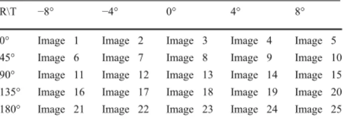
To calibrate an experimental setup, images are acquired of the micro scale grid at various orientations. During the calibration process, the specimen is moved as necessary to maintain adequate focus. Table7presents the experimental out of plane rotations and in plane rotations used to acquire 25 images of the micro grid for calibration. Out of plane specimen rotations from 8° to 8° are performed using the eucentric goniometer. In plane specimen rotations are performed using a built in Quanta 200 electron beam rotation function.

Experimental Phase

Once the distortion correction process and the calibration procedure have been completed, all SEM settings are maintained and the specimen is placed on the eucentric goniometer in the SEM chamber. Prior to applying load, images of the planar speckled specimen rotated out of plane by 10° and +10°, respectively, are acquired as the reference image pair.

Loading is applied to the specimen and images are acquired with the specimen oriented at 10° and +10° respectively. This process of out of plane specimen rotation and incremental loading is repeated until the experiment is completed.

Image Processing

After completing the three primary phases of the experi mental work, images are evaluated from each phase.8First, the spatial distortion correction images are processed using procedures outlined previously [32] for optical image correction. Second, all calibration images are analyzed to obtain the center point position of each grid point. Each identified grid point is corrected for spatial distortion and bundle adjustment procedures within VIC 3D are used to obtain (a) the intrinsic parameters for the SEM stereo vision

system and (b) the orientation and position of each calibration grid.

Finally, all speckle images for the 10° and +10° specimen rotations are corrected for spatial distortion and then input into VIC 3D as stereo image pairs for cross correlation and three dimensional motion measurements.

References

1. Chasiotis I (2004) Mechanics of thin films and microdevices. IEEE Trans on Device and Mater Reliab 4(2):176 188

2. Hemker KJ, Sharpe WN (2007) Microscale characterization of mechanical properties. Annu Rev Mater Res 37:93

3. Sharpe WN (2003) Murray lecture tensile testing at the micrometer scale: Opportunities in Exp Mech. Exp Mech 43 (3):228 237

4. Sutton MA, Li N, Garcia D et al (2006) Metrology in a scanning electron microscope: theoretical developments and experimental validation. Meas Sci & Tech 17(10):2613 2622

5. Kang J, Ososkov J, Embury J et al (2007) Digital image correlation studies for microscopic strain distribution and damage in dual phase steels. Scr Mater 56(11):999 1002

6. Sabate N, Vogel D, Gollhardt A et al (2006) Digital image correlation of nanoscale deformation fields for local stress measurement in thin films. Nanotechnol 17(20):5264

7. Bao G, Suresh S (2003) Cell and molecular mechanics of biological materials. Nat Mater 2(11):715 725

8. Chen CS, Mrksich M, Huang S et al (1997) Geometric control of cell life and death. Sci 276(5317):1425

9. Dikovsky D, Bianco Peled H, Seliktar D (2008) Defining the role of matrix compliance and proteolysis in three dimensional cell spreading and remodeling. Biophys J 94(7):2914

10. Pedersen JA, Swartz MA (2005) Mechanobiology in the third dimension. Ann of Biomed Eng 33(11):1469 1490

11. Yeung T, Georges PC, Flanagan LA et al (2005) Effects of substrate stiffness on cell morphology, cytoskeletal structure, and adhesion. Cell Motil Cytoskelet 60(1):24 34

12. Marinello F, Bariani P, Savio E et al (2008) Critical factors in SEM 3D stereo microscopy. Meas Sci Tech 19(6):65705 13. Raspanti M, Binachi E, Gallo I et al (2005) A vision based, 3D

reconstruction technique for scanning electron microscopy: direct comparison with atomic force microscopy. Microsc Res Tech 67 (1):1

14. Ponz E, Ladaga JL, Bonetto RD (2005) Measuring surface topography with scanning electron microscopy. I. EZEImage: a program to obtain 3D surface data. Microsc and Microanal 12 (02):170 177

8_{All image analyses were performed using a modified version of} VIC 3D commercial software,www.correlatedsolutions.com

Table 7 Image sequence for calibration

R\T −8° −4° 0° 4° 8°

0° Image 1 Image 2 Image 3 Image 4 Image 5

45° Image 6 Image 7 Image 8 Image 9 Image 10

90° Image 11 Image 12 Image 13 Image 14 Image 15 135° Image 16 Image 17 Image 18 Image 19 Image 20 180° Image 21 Image 22 Image 23 Image 24 Image 25 R is the in plane e beam rotation angle

T is the specimen rotation angle for the eucentric goniometer within the FEI Quanta 200

15. Villarrubia JS, Vladar AE, Postek MT (2005) Scanning electron microscope dimensional metrology using a model based library. Surf Interface Anal 37(11):951 958

16. Bariani P, De Chiffre L, Hansen HN et al (2005) Investigation on the traceability of three dimensional scanning electron microscope measurements based on the stereo pair technique. Precis Eng 29 (2):219 228

17. Sinram O, Ritter M, Kleindiek S et al (2002) Calibration of an SEM, using a nano positioning tilting table and a microscopic calibration pyramid. Int Arch Photogramm Remote Sens Spat Info Sci 34(5):210 215

18. Scherer S (2002) 3D surface analysis in scanning electron microscopy. GIT Imaging Microsc 3:45 46

19. Scherer S, Werth P, Pinz A et al (1999) Automatic surface reconstruction using SEM images based on a new computer vision approach. Inst of Phys Pub Inc

20. Password F (1999) Three dimensional morphometry in scanning electron microscopy: a technique for accurate dimensional and angular measurements of microstructures using stereopaired digitized images and digital image analysis. J Microsc 195(1):23 33 21. Kayaalp AE, Rao AR, Jain R (1990) Scanning electron

microscope based stereo analysis. Mach Vis App 3(4):231 246 22. Kolednik O (1981) A contribution to stereophotogrammetry with

the scanning electron microscope. Prakt Metallogr 18(12):562 573 23. Boyde A, Ross HF (1975) Photogrammetry and the scanning

electron microscope. Photogramm Rec 8(46):408 408

24. Piazzesi G (1973) Photogrammetry with the scanning electron microscope. J Phys E Sci Instrum 6:392 396

25. Maune DF (1973) Photogrammetric self calibration of a scanning electron microscope. Univ Microfilm Int

26. MeX software; Alicona Imaging;www.alicona.com

27. Lockwood WD, Reynolds AP (1999) Use and verification of digital image correlation for automated 3 d surface characteriza tion in the scanning electron microscope. Mater Charact 42(2 3):123 134

28. Faugeras O, Luong QT, Papadopoulo T (2001) The geometry of multiple images. MIT, Cambridge

29. Sutton MA, Li N, Joy DC et al (2007) Scanning electron microscopy for quantitative small and large deformation measure

ments part I: SEM imaging at magnifications from 200 to 10, 000. Exp Mech 47(6):775 787

30. Sutton MA, Li N, Garcia D et al (2007) Scanning electron microscopy for quantitative small and large deformation measure ments Part II: experimental validation for magnifications from 200 to 10, 000. Exp Mech 47(6):789 804

31. Sutton MA, Orteu JJ, Schreier HW (2009) Image correlation for shape, motion and deformation measurements: basic concepts, theory and practical applications. Springer, New York. ISBN 978 0 387 78747 3

32. Sutton MA, Correlation DI, Sharpe WN Jr (eds) (2008) Springer handbook of experimental solid mechanics. Springer, Berlin. ISBN 978 0 387 26883 5

33. Faugeras O (1993) Three dimensional computer vision: a geo metric viewpoint. MIT, Cambridge

34. Helm JD, McNeill SR, Sutton MA (1996) Improved three dimensional image correlation for surface displacement measure ment. Opt Eng 35:1911

35. Schreier HW, Garcia D, Sutton MA (2004) Advances in light microscope stereovision. Exp Mech 44(3):278 288

36. Triggs B, McLauchlan P, Hartley R et al (1999) Bundle Adjustment A modern synthesis. Lecture notes in computer science. p. 298 372

37. Schreier HW, Sutton MA (2002) Systematic errors in digital image correlation due to undermatched subset shape functions. Exp Mech 42(3):303 310

38. Schreier HW, Braasch JR, Sutton MA (2000) Systematic errors in digital image correlation caused by intensity interpolation. Opt Eng 39:2915

39. Wang YQ, Sutton MA, Schreier HW (2009) Quantitative error assessment in pattern matching: effects of intensity pattern noise, interpolation, strain and image contrast on motion measurements quantitative error assessment in pattern matching: effects of intensity pattern noise, interpolation, strain and image contrast on motion measurements. J Strain 45:160 178

40. VIC 2D and VIC 3D, Correlated Solutions Inc., West Columbia, SC,www.correlatedsolutions.com