Science Arts & Métiers (SAM)
is an open access repository that collects the work of Arts et Métiers Institute of Technology researchers and makes it freely available over the web where possible.
This is an author-deposited version published in: https://sam.ensam.eu Handle ID: .http://hdl.handle.net/10985/17477
To cite this version :
Peng WANG, Hocine CHALAL, Farid ABED-MERAIM - Quadratic solidshell elements for nonlinear structural analysis and sheet metal forming simulation - COMPUTATIONAL MECHANICS - Vol. 59, n°1, p.161–186 - 2017
Any correspondence concerning this service should be sent to the repository Administrator : archiveouverte@ensam.eu
1
Quadratic solid‒shell elements for nonlinear structural
analysis and sheet metal forming simulation
Peng WANG, Hocine CHALAL, Farid ABED-MERAIM
LEM3, UMR CNRS 7239 - Arts et Métiers ParisTech, 4, rue Augustin Fresnel, 57078 Metz Cedex 03, France
Abstract In this paper, two quadratic solid‒shell (SHB) elements are proposed for the three-dimensional modeling of thin structures. These consist of a twenty-node hexahedral solid‒shell element, denoted SHB20, and its fifteen-node prismatic counterpart, denoted SHB15. The formulation of these elements is extended in this work to include geometric and material nonlinearities, for application to problems involving large displacements and rotations as well as plasticity. For this purpose, the SHB elements are coupled with large-strain anisotropic elasto-plastic constitutive equations for metallic materials. Although based on a purely three-dimensional approach, several modifications are introduced in the formulation of these elements to provide them with interesting shell features. In particular, a special direction is chosen to represent the thickness, along which a user-defined number of integration points are located. Furthermore, for efficiency requirements and for alleviating locking phenomena, an in-plane reduced-integration scheme is adopted. The resulting formulations are implemented into the finite element software ABAQUS/Standard and, to assess their performance, a variety of nonlinear benchmark problems are investigated. Attention is then focused on the simulation of various complex sheet metal forming processes, involving large strain, anisotropic plasticity, and double-sided contact. From all simulation results, it appears that the SHB elements represent an interesting alternative to traditional shell and solid elements, due to their versatility and capability of accurately modeling selective nonlinear benchmark problems as well as complex sheet metal forming processes.
Keywords finite element, quadratic solid‒shell, thin structures, nonlinear analysis, anisotropic plasticity, sheet metal forming.
2
1 Introduction
Nowadays, the numerical modeling has become an indispensable simulation tool in many fields of the industry, such as automotive, aerospace, and civil engineering. The finite element (FE) method, a widespread numerical tool, provides great assistance to engineers in the design of products and optimization of manufacturing processes. Despite the growing development of computational resources, reliability and efficiency of the FE analysis remain important features in the simulation practice. The present work deals with the simulation of thin structures, which is conventionally achieved using classical shell and continuum solid elements. However, in some circumstances, traditional shell and solid elements suffer from various locking phenomena, such as membrane locking, thickness locking, shear locking, etc. In addition, shell elements are often not appropriate for the modeling of complex sheet metal forming processes involving double-sided contact, partly due to the use of plane-stress assumptions in their formulation. To remedy these shortcomings, considerable effort has been devoted to the development of solid‒shell elements during the last few decades. The key idea behind this original concept of solid‒shell elements is to combine the advantages of both FE technologies, namely shell and continuum formulations. The main benefits of this solid‒shell concept may be summarized as follows: easier formulation, based on a purely three-dimensional approach, with displacements as the only degrees of freedom; consideration of fully three-dimensional constitutive laws, with no plane-stress restrictions; direct calculation of thickness variations; natural treatment of double-sided contact, thanks to the availability of actual top and bottom surfaces; 3D modeling of thin structures, using only a single element layer and few integration points, while accurately describing the through-thickness phenomena.
Most solid‒shell elements developed in the literature are based on the reduced-integration technique (see, e.g., Zienkiewicz et al. [1]). In the case of linear interpolation, this consists most often in adopting an in-plane one-point quadrature rule, while considering a number of integration points along the thickness. In addition to the reduced-integration scheme, several other numerical strategies, such as the assumed strain method (ASM), the enhanced assumed strain (EAS) approach, the assumed natural strain (ANS) concept, were developed in the literature to eliminate various kinds of locking phenomena (see, e.g., [2‒17]). Note that, for linear under-integrated solid‒shell elements, special stabilization procedures are required for the control
3
of zero-energy (hourglass) modes, which are induced by the reduced-integration rule (see, e.g., Abed-Meraim and Combescure [12], Schwarze et al. [18]).
In this paper, two quadratic solid‒shell elements are proposed for the 3D nonlinear analysis of thin structures. These formulations are extended to include geometric and material nonlinearities, following the earlier works on the family of SHB elements. The first solid‒shell element in this family was developed by Abed-Meraim and Combescure [6], and consists of an eight-node hexahedral element denoted SHB8PS. Its formulation was subsequently improved by Abed-Meraim and Combescure [12], especially in terms of locking reduction, while the hourglass modes were efficiently controlled by implementing a new stabilization procedure. The performance of the SHB8PS element was demonstrated through a representative set of selective benchmark tests as well as sheet metal forming processes involving large strains, anisotropic plasticity, and contact (see Abed-Meraim and Combescure [12], Salahouelhadj et al. [19]). Then, a six-node prismatic solid‒shell element denoted SHB6 was developed by Trinh et al. [20], as a complement to the SHB8PS element for the modeling of complex geometries whose meshing requires the combination of hexahedral and prismatic elements. Although the performance of the SHB6 is good in the whole, its convergence rate remains slower than that of the SHB8PS, and requires finer meshes to obtain accurate solutions. More recently, the quadratic counterparts of the above hexahedral and prismatic solid‒shell elements were developed by Abed-Meraim et al. [21], in order to improve the overall performance and convergence rate. These quadratic versions consist of a twenty-node hexahedral element, denoted SHB20, and a fifteen-node prismatic element, denoted SHB15. Likewise, their formulation is based on a fully three-dimensional approach with an in-plane reduced-integration rule. The performance of these elements has been evaluated by Abed-Meraim et al. [21] within the framework of small strain and elastic benchmark problems. In the present work, however, the formulation of the quadratic SHB15 and SHB20 elements is extended to the framework of large displacements and rotations. Moreover, the resulting formulations are coupled with large-strain anisotropic elasto-plastic constitutive equations, which allows modeling complex and challenging structural problems, such as sheet metal forming processes.
The remainder of the paper is outlined as follows. The general formulation of the quadratic solid‒shell elements, SHB15 and SHB20, is presented in Section 2. Then, the performance of these elements is assessed in Section 3, first through a variety of linear and nonlinear benchmark
4
problems. In Section 4, the proposed formulations are applied to the simulation of complex sheet metal forming processes, including springback, incremental forming, and deep drawing tests. Finally, the main conclusions and remarks are drawn in Section 5.
2 Basic formulations for the quadratic solid‒shell elements
Despite some differences between the prismatic and hexahedral solid‒shell elements (e.g., in terms of geometry, interpolation functions, etc.), their theoretical formulations show a number of similarities. In this section, a general formulation, common to both SHB15 and SHB20 solid‒shell elements, is introduced. This formulation, which was previously developed by Abed-Meraim et al. [21] within the framework of small strains, is extended here to the large-strain framework.
2.1 Geometry and integration points
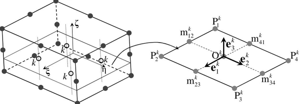
Figure 1 illustrates the reference geometry and location of integration points for the SHB15 and SHB20 solid‒shell elements. The starting point for the formulation of these quadratic solid‒shell elements is the classical 3D approach, used for conventional quadratic continuum elements, with fifteen nodes for the prismatic SHB15 element and twenty nodes for the SHB20 element. Then, a special direction ζ (see Fig. 1) is chosen as the thickness direction, along which a user-defined number of integration points are arranged. In the ξ η− plane corresponding to each ζ -coordinate of these through-thickness integration points, are defined a total number of three integration points for the prismatic SHB15 element, and four integration points for the hexahedral SHB20 element, as shown in Fig. 1. The coordinates and associated weights of these integration points can be obtained using the classical Gauss distribution method (see, e.g., Zienkiewicz et al. [22]). It is worth noting that, in the case of full integration for conventional quadratic solid elements, three in-plane integration points with three through-thickness integration points are required for prismatic elements, while nine in-plane integration points with three through-thickness integration points are used for hexahedral elements.
5
(a) SHB15 (b) SHB20
Fig. 1. Reference geometry and location of integration points for the SHB15 and SHB20 solid‒shell elements.
Moreover, to provide the proposed elements with some desirable shell features and to reduce locking, special local element frames are introduced, which are attached to the element mid-planes associated with each integration point. In these local physical coordinate systems, associated with the ζ -coordinate of each integration point, the fully three-dimensional elasticity tensor of the material is specified. Note that this is a first major difference with conventional continuum elements, for which no such local element frames are considered. Figure 2 illustrates, in the case of the SHB20 element, the definition of these local element frames, which are built using the following procedure. First, the element mid-plane corresponding to a given integration point k is defined using the physical nodal coordinates, which is represented in Fig. 2 by the four points
P
1k,P
2k,P
3k andP
4k. These latter points allow us, in turn, to define four mid-points m , 12kk 23 m , k 34 m and k 41
m , which are the barycenters of
(
P P
1k 2k)
,(
P P
2k 3k)
,(
P P
3k 4k)
and(
P P
4k 1k)
, respectively. Then, the first base vector, k1
e , of the local coordinate system is defined as being parallel to
(
m
41km
23k)
, while the second vector e is defined parallel to k2(
m m
12 34)
k k
. Vector e2k is modified by adding a correction term ekc, so that vectors e and 1k
(
2)
k k
c
+
e
e
are orthogonal, which gives6
( )
( )
1 2 1 1 1 T k k k k c k T k ⋅ = − ⋅ e e e e e e . (1)Finally, the third base vector e is simply obtained by the following cross-product (see Fig. 2): k3
(
)
3 1 2 k k k k c = × + e e e e . (2)The same strategy is applied to the prismatic SHB15 element, in order to define the associated local coordinate systems, and is not repeated here for conciseness.
k k k k k
e
k2 1e
k 12m
k 23m
mk34 k 41 m k 1 P k 2 P k 3 P k 4 P k 3e
ζ ξ η k OFig. 2. Schematic representation of the local element frame associated with the kth integration point of the SHB20 element.
2.2 Quadratic interpolation for the SHB elements
Using the classical isoparametric approach, the SHB15 and SHB20 solid‒shell elements adopt the conventional shape functions N for quadratic prismatic and hexahedral elements, I
respectively. The spatial coordinates x and the displacement field i u within the element are i
expressed as functions of the nodal coordinates and the nodal displacement, respectively
∑
= = = n I iI I I iI i x N N x x 1 ) , , ( ) , , (ξ η ζ ξ η ζ , (3) ) , , (ξη ζ I iI i d N u = , (4)7
where the lowercase subscript i varies from 1 to 3, and represents the spatial coordinate directions, while the uppercase subscript I goes from 1 to n, with n being the number of element nodes (n=15 for the SHB15 element, and n=20 for the SHB20 element). Note that in Eq. (4) above, the convention of implied summation over repeated indices has been used, which will be also adopted in the sequel.
2.3 Strain-displacement relationship and discrete gradient operator
Based on the interpolation of the displacement field (Eq. (4)), the linear part ε of the strain tensor is defined by the following relationship:
(
i j ji) (
iI I j jI I i)
ij = u, +u, = d N , +d N , 2 1 2 1 ε . (5)The combination of Eqs. (3) and (4), along with the expression of the shape functions )
, , (ξ η ζ
I
N ,allows us to develop the displacement field in the following form:
0 1 1 2 2 3 3 1 1 2 2
i i i i i i i i
u =a +a x +a x +a x +c h +c h + +⋯ c hα α, (6) where hα are functions of the nodal coordinates ξ, η, ζ , in the reference coordinate system, and α varies from 1 to 11 for the SHB15 element, and from 1 to 16 for the SHB20 element. For the SHB15 element, the hα functions are expressed as follows:
2 2 2 1 2 3 4 5 6 7 2 2 2 2 8 9 10 11 , , , , , , , , , , , h h h h h h h h h h h ξζ ηζ ξη ξηζ ξ η ζ ξ ζ η ζ ξζ ηζ = = = = = = = = = = = (7)
while for the SHB20 element, they are given by
2 2 2 1 2 3 4 5 6 7 2 2 2 2 2 2 8 9 10 11 12 13 2 2 2 14 15 16 , , , , , , , , , , , , , , , . h h h h h h h h h h h h h h h h ξζ ηζ ξη ξ η ζ ξηζ ξ η ξ ζ η ξ η ζ ξζ ηζ ξ ηζ ξη ζ ξηζ = = = = = = = = = = = = = = = = (8)
By evaluating Eq. (6) at the fifteen nodes of the SHB15 element, respectively, at the twenty nodes of the SHB20 element, one obtains the following fifteen-equation system, respectively, twenty-equation system: α αh h h x x x s di =a0i +a1i 1+a2i 2+a3i 3+c1i 1+c2i 2+⋯+ci , i=1, 2, 3, (9)
8
where dTi =
(
di1,di2,di3,⋯,din)
represent the nodal displacement vectors, and(
i i i in)
T
i = x1,x2,x3,⋯,x
x are the nodal coordinate vectors. The constant vector sT =
(
1, 1,⋯, 1)
is a fifteen-component vector, in the case of the SHB15 element, and a twenty-component vector, for the SHB20 element. As to vectors h , these are constant vectors whose expressions can be α easily obtained by evaluating the hα functions at the element nodes in the reference coordinate system ( , , )ξ η ζ (for the full details, see Abed-Meraim et al. [21]).By introducing the Hallquist [23] vectors
| 0 i i x ξ η ζ= = = ∂ = ∂ N
b , with N the vector whose
components are the shape functions N , one can demonstrate the following first set of I
orthogonality conditions, which is common to both elements: 0 0 T i T i T i j ij α
δ
⋅ = ⋅ = ⋅ = b h b s b x , (10)where ,i j=1, 2, 3, while α =1,...,11, for the SHB15 element, and α =1,...,16, for the SHB20 element.
Then, a second set of orthogonality conditions are established for the SHB15 element
1 9 2 10 3 11 4 5 6 7 8 = 0, = 0 = 0, = 4 1 = , = 4 2 = 0 = 4 = 4 = 12 = 0 T T T T T T T T T T T ⋅ ⋅ ⋅ ⋅ ⋅ ⋅ ⋅ ⋅ ⋅ ⋅ ⋅ h s h s h s h s h s h s h s h s h s h s h s , (11)
9 1 9 2 10 3 11 4 12 5 13 6 14 7 15 8 16 = 0, = 0 = 0, = 0 = 0, = 0 = 16, = 0 = 16, = 0 = 16, = 0 = 0, = 0 = 0, = 0 T T T T T T T T T T T T T T T T ⋅ ⋅ ⋅ ⋅ ⋅ ⋅ ⋅ ⋅ ⋅ ⋅ ⋅ ⋅ ⋅ ⋅ ⋅ ⋅ h s h s h s h s h s h s h s h s h s h s h s h s h s h s h s h s . (12)
Using the above orthogonality conditions (Eqs. (10‒12)), and the scalar product of Eq. (9) by
T j
b , sT and hTα, successively, the expression of the unknown constants aji and cαi in Eqs. (6) and
(9)can be obtained as follows:
i T i i T j ji c a =b ⋅d, α =γα ⋅d , (13)
where the expressions of vectors γ for the SHB15 element are given by α
(
)
(
)
(
(
)
)
(
)
(
)
1 1 1 2 2 2 3 3 3 4 4 4 5 5 5 6 6 6 1 1 30 30 4 4 4 4 15 15 15 15 T T T T T T T j j j j T T T T T T T T j j j j T T T T T T T T T j j j L L L L L L α α α α α α α = − ⋅ + − ⋅ + − − − ⋅ + − ⋅ + − − − ⋅ + − − − ⋅ γ h h x b h h x b h s h s x b h h x b h s h s x b h s h s x(
)
(
)
(
)
(
)
7 7 7 8 8 8 9 9 9 10 10 10 11 11 11 4 4 5 5 4 4 15 15 4 4 15 15 T j T T T T T T T T j j j j T T T T T T T T j j j j T T T T j L L L L L α α α α α + − − − ⋅ + − ⋅ + − ⋅ + − − − ⋅ + − − − ⋅ b h s h s x b h h x b h h x b h s h s x b h s h s x Tj b with10 17 0 0 8 0 0 0 9 0 0 0 2 17 0 0 8 0 0 0 0 9 0 0 2 256 36 36 58 58 0 0 0 2 0 0 17 17 17 17 17 8 8 0 24 0 0 0 8 8 0 0 36 316 146 324 171 0 0 0 1 0 0 17 187 187 187 187 36 146 316 171 324 0 0 0 1 0 0 17 187 187 187 187 3 3 3 0 0 2 0 1 1 0 0 2 2 2 9 0 0 8 0 0 0 10 0 0 0 0 9 0 8 0 0 0 0 10 0 0 58 0 0 0 17 αβ − − − − − − − − − − − − − − − − − − = L 324 171 3 505 585 0 0 187 187 2 187 374 58 171 324 3 585 505 0 0 0 0 0 17 187 187 2 374 187 , 1, ..., 11
α β
− − − − − − =while for the SHB20 element, vectors γ are given by α
(
)
(
)
(
(
)
)
(
)
(
)
1 1 1 2 2 2 3 3 3 4 4 4 5 5 5 6 6 6 4 4 5 5 4 4 4 4 5 5 5 5 T T T T T T T j j j j T T T T T T T T j j j j T T T T T T T T T j j j j L L L L L L α α α α α α α = − ⋅ + − ⋅ + − ⋅ + − − − ⋅ + − − − ⋅ + − − − ⋅ γ h h x b h h x b h h x b h s h s x b h s h s x b h s h s x b(
)
(
)
(
(
)
)
(
)
(
)
(
(
)
)
(
)
(
)
(
(
)
)
(
)
(
)
(
(
)
)
(
)
(
)
(
(
)
)
7 7 7 8 8 8 9 9 9 10 10 10 11 11 11 12 12 12 13 13 13 14 14 14 15 15 15 16 16 16 T T T T T T T j j j j T T T T T T j j j j T T T T T T j j j j T T T T T T j j j j T T T T T T j j j j L L L L L L L L L L α α α α α α α α α α + − ⋅ + − ⋅ + − ⋅ + − ⋅ + − ⋅ + − ⋅ + − ⋅ + − ⋅ + − ⋅ + − ⋅ h h x b h h x b h h x b h h x b h h x b h h x b h h x b h h x b h h x b h h x b11 with 1 1 0 0 0 0 0 0 0 0 0 0 0 0 0 0 4 4 1 1 0 0 0 0 0 0 0 0 0 0 0 0 0 0 4 4 1 1 0 0 0 0 0 0 0 0 0 0 0 0 0 0 4 4 3 1 1 0 0 0 0 0 0 0 0 0 0 0 0 0 8 8 8 1 3 1 0 0 0 0 0 0 0 0 0 0 0 0 0 8 8 8 1 1 3 0 0 0 0 0 0 0 0 0 0 0 0 0 8 8 8 1 0 0 0 0 0 0 0 0 0 0 0 0 0 0 0 8 3 1 0 0 0 0 0 0 0 0 0 0 0 0 0 0 20 10 3 1 0 0 0 0 0 0 0 0 0 0 0 0 0 0 20 10 3 1 0 0 0 0 0 0 0 0 0 0 0 0 0 0 20 10 0 0 αβ − − − − − − = L 1 3 0 0 0 0 0 0 0 0 0 0 0 0 10 20 1 3 0 0 0 0 0 0 0 0 0 0 0 0 0 0 10 20 1 3 0 0 0 0 0 0 0 0 0 0 0 0 0 0 10 20 1 1 0 0 0 0 0 0 0 0 0 0 0 0 0 0 4 8 1 1 0 0 0 0 0 0 0 0 0 0 0 0 0 0 4 8 1 1 0 0 0 0 0 0 0 0 0 0 0 0 0 0 4 8 ,
α β
− − − − − − =1, ..., 16By differentiating Eq. (6) and using Eq. (13), the expression of the displacement gradient ui j,
is derived as follows:
(
)
, , T T i j j j i u = b +hα γα ⋅d , (14)12
with α varying from 1 to 11 for the SHB15 element, and from 1 to 16 for the SHB20 element. Finally, the expression of the strain field, which is related to the nodal displacements by the discrete gradient operator B , is given by
( )
⋅ = ⋅ = + + + = ∇ z y x x z z x y z z y x y y x z z y y x x s u u u u u u u u u d d d B d B u , , , , , , , , , , (15)where the discrete gradient operator B takes the following matrix form:
+ + + + + + + + + = T x T x T z T z T y T y T z T z T x T x T y T y T z T z T y T y T x T x h h h h h h h h h α α α α α α α α α α α α α α α α α α γ b 0 γ b γ b γ b 0 0 γ b γ b γ b 0 0 0 γ b 0 0 0 γ b B , , , , , , , , , . (16) 2.4 Variational principle
The assumed-strain formulation of the SHB15 and SHB20 solid‒shell elements is based on the simplified form of the Hu‒Washizu mixed variational principle, as suggested by Simo and Hughes [24], which writes at the element level
0 = ⋅ − Ω ⋅ =
∫
Ω T T ext e d d f σ ε εɺ δɺ δɺ δπ( ) , (17)where δ denotes a variation, εɺ the assumed-strain rate, σ the Cauchy stress tensor, dɺ the nodal velocities, and fext the external nodal forces. It is worth noting that in the formulation of the linear versions of the solid‒shell elements (i.e., SHB6 and SHB8PS, see, e.g., Abed-Meraim and Combescure [12], Trinh et al. [20]), the assumed-strain rate εɺ has been expressed in terms of a projected matrix B , which is derived from the classical B operator, in order to eliminate most locking phenomena (e.g., membrane locking, shear locking, etc.). For the present quadratic solid‒shell elements (SHB15 and SHB20), no significant locking has been revealed when
13
evaluating their performance on a selective and representative set of benchmark problems (see Abed-Meraim et al. [21]). Consequently, no projection is applied to the discrete gradient operator
B and, accordingly, the expression of the assumed-strain rate reduces to d
B
εɺ(x,t)= ⋅ɺ. (18)
Substituting the above equation into the simplified form of the Hu‒Washizu variational principle, the expressions of the element stiffness matrix and internal force vector are obtained as follows:
∫
∫
Ω ⋅ ⋅ Ω = Ω ⋅ Ω = e e d d T T e , ( ) int ε σ B f B C B K ep ɺ , (19)where C is the fourth-order elasto-plastic tangent modulus, whose expression will be detailed ep in the following subsection.
2.5 Constitutive equations
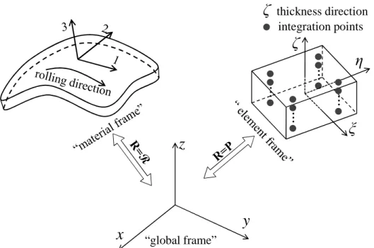
The formulation of the quadratic solid‒shell elements SHB15 and SHB20 is extended in this paper to the framework of large displacements and rotations, and is coupled with advanced large-strain anisotropic constitutive equations for metallic materials. In this process, two types of local frames need to be introduced with respect to the global coordinate system, as illustrated in Fig. 3. The first type of local frame, which has already been defined in Section 2.1 (see Fig. 2) and denoted as the “element frame”, is attached to the element mid-plane associated with each integration point. The second type of local physical coordinate system is the so-called “material frame”, which is introduced to define the anisotropic plastic behavior of the material. The time integration of the large-strain anisotropic elasto-plastic constitutive equations, which is achieved at each integration point, also uses this local material frame in order to satisfy the objectivity (material invariance) requirements. Both the local element frame and the material frame are defined relative to the global coordinate frame by their rotation matrix P and R, respectively, which allows mapping any vector a or tensor A from local to global coordinate systems.
14
z
y
x
“global frame”...
η
ξ
ζ
...
...
...
ζ
thickness direction integration pointsFig. 3. Illustration of the local coordinate systems used in the formulation of the quadratic solid‒shell elements.
For the modeling of the anisotropic plastic behavior, the quadratic Hillʼ48 yield criterion [25] is coupled with the formulation of the SHB elements. Accordingly, the plastic yield function is given by
(
)
(
)
YF= σ′−α :M: σ′−α − , (20)
where σ′ denotes the deviatoric part of the Cauchy stress tensor σ , and α is the back-stress
tensor, which describes the kinematic hardening of the material. The fourth-order tensor M contains the Hill anisotropy coefficients (F, G, H, L, M and N). The isotropic hardening of the material, which characterizes the size of the yield surface, is modeled by the scalar function Y .
The plastic strain rate tensor D is obtained using the classical associative plastic flow rule, p which follows the normality law with respect to the yield surface
p λ∂F λ = = ∂ D V σ ɺ ɺ , (21)
15
In the local material frame, the Cauchy stress rate can be expressed using the following hypo-elastic law:
(
)
e p
= : −
σɺ C D D , (22)
where the second-order tensor D denotes the total strain rate, while C is the fourth-order e elasticity tensor. Note that a modified plane-stress-type elasticity matrix has been adopted in the formulation of the linear versions of the SHB elements (see, e.g., Abed-Meraim and Combescure [12], Trinh et al. [20]), in order to avoid the locking phenomena encountered when the classical fully three-dimensional elasticity tensor is considered. By contrast, such a modification is not required for the present quadratic versions of the SHB elements, since their performance has been assessed with both the plane-stress-type elasticity matrix and the classical fully three-dimensional one, showing quite equivalent results. Therefore, the classical fully three-dimensional elasticity matrix is implemented with the proposed quadratic versions of the SHB elements, which represents a major advantage with respect to their linear counterparts.
The plastic multiplier λɺ in Eq. (21) is determined by using the consistency condition Fɺ =0, which leads to e e : : λ : : : HY = + α+ V C D V C V V H ɺ , (23)
where the hardening moduli H and Y Hα are scalar and tensor components involved in the evolution laws describing the isotropic and kinematic hardening, respectively. The latter can be expressed in the following generic form:
λ λ Y Y H = = α Hα ɺ ɺ ɺ ɺ . (24)
Finally, by substituting the expression of the plastic multiplier λɺ into the hypo-elastic law (22), the elasto-plastic tangent modulus is derived as
(
e) (
e)
ep e e : : : : : HY ⊗ = − γ + α+ C V V C C C V C V V H , (25)16
3 Simulation of linear and nonlinear benchmark problems
The formulations of the quadratic solid‒shell elements (SHB15 and SHB20) presented above have been implemented into the finite element code ABAQUS/Standard. A representative set of linear and nonlinear benchmark tests is selected in this section to evaluate the performance of the proposed SHB elements. The obtained results are systematically compared, on the one hand, with those provided by ABAQUS quadratic elements, using the same in-plane meshes, and on the other hand with reference solutions taken from the literature. The description of the finite elements used for comparison purposes is given in Table 1. Note that, for the proposed SHB15 and SHB20 formulations, only two integration points along the thickness are sufficient to model the following linear and nonlinear elastic benchmark tests, while three integration points are used in the case of elasto-plastic benchmark problems.
In this section, all geometries are discretized using the following nomenclature. For hexahedral elements, meshes of N1×N2×N3 elements are adopted, where N1 denotes the number
of elements in the length direction, N2 is the number of elements in the width direction, and N3 is
the number of elements in the thickness direction. For meshes with prismatic elements, the nomenclature adopted is (N1×N2×2)×N3, which corresponds to twice the total number of
elements involved in hexahedron-based meshes, due to the subdivision of each hexahedron into two prisms. For ABAQUS shell elements, the nomenclature adopted for quadrilateral shell elements is N1×N2, while the nomenclature for triangular shell elements is N1×N2×2.
17
Table 1
Quadratic prismatic, hexahedral, and shell finite elements used in the simulations.
Prismatic elements / Triangular shell element
SHB15 15-node prismatic solid‒shell element with a user-defined number of through-thickness integration points C3D15 15-node prismatic solid element with three integration
points through the thickness
STRI65 6-node triangular shell element with a user-defined number of through-thickness integration points
Hexahedral elements / Quadrilateral shell
element
SHB20 20-node hexahedral solid‒shell element with a user-defined number of through-thickness integration points C3D20 20-node hexahedral solid element with three
integration points through the thickness S8R
8-node reduced-integration quadrilateral shell element with a user-defined number of through-thickness integration points
3.1 Bending of a clamped square plate
The performance of the proposed SHB elements is first evaluated on a linear elastic problem, which consists of a clamped square plate subjected to a central concentrated force. The geometric dimensions, material properties, and boundary conditions of the problem are all illustrated in Fig. 4. The value of the concentrated point load is chosen so that the analytical displacement at the center of the plate is
2 FL 0.0056 1 ref u D = = , where ) ( 2 3 1 12 t v E D −
= is the flexural rigidity of the
plate [26]. Owing to the symmetry, only one quarter of the plate is discretized using three different regular meshes, in order to assess the convergence rate of the proposed SHB elements. The convergence results for the SHB elements, in terms of central point displacement normalized with respect to the analytical displacement uref =1, are shown in Fig. 5 along with the results given by ABAQUS quadratic elements. Among the prismatic and triangular elements, the ABAQUS quadratic shell element STRI65 has the fastest convergence, followed by the proposed SHB15 element, while the convergence of the ABAQUS quadratic solid element C3D15 is the slowest. For the hexahedral and quadrilateral elements, the convergence of the proposed SHB20 element is similar to that of the ABAQUS quadratic shell element S8R, which is much faster than that of the ABAQUS quadratic solid element C3D20.
18 clamped E = 10000 v = 0.3 L = 100 t = 1 F = 16.3527 F
Fig. 4. Geometry, material properties, and boundary conditions for the clamped square plate.
0.2 0.4 0.6 0.8 1.0 (8×8×2)×1 (4×4×2)×1 D is p la ce m en t Number of elements Analytical solution SHB15 C3D15 STRI65 (2×2×2)×1 0.2 0.4 0.6 0.8 1.0 8×8×1 4×4×1 D is p la ce m en t Number of elements Analytical solution SHB20 C3D20 S8R 2×2×1
(a) triangular shell / prismatic elements (b) quadrilateral shell / hexahedral elements Fig. 5. Convergence results for the clamped square plate subjected to a central concentrated force.
In addition to the convergence results above, a sensitivity analysis with respect to the in-plane mesh distortion is conducted here, as proposed by Alves de Sousa et al. [8]. To this end, a quarter of the square plate is discretized by (2×2×2)×1 elements, in the case of triangular shell or prismatic elements, and by 2×2×1 elements, in the case of quadrilateral shell or hexahedral elements. The mesh distortion is created by moving the central node of the mesh (see point B in Fig. 6) with a predefined distance d ( 0≤ ≤d 12), as illustrated in Fig. 6. Again, the normalized displacement of the central point A (see Fig. 6), as a function of the distortion parameter d , is investigated. Figure 7 shows the effect of the distortion parameter d on the normalized displacement of the central point A, as obtained with the SHB elements and ABAQUS quadratic
19
solid and shell elements. With regard to mesh distortion sensitivity, the ABAQUS triangular shell element STRI65 shows better performance than the SHB15 element; nevertheless, the latter performs better than the ABAQUS prismatic solid element C3D15. For the hexahedral elements, the sensitivity of the proposed SHB20 element to mesh distortion is similar to that displayed by the ABAQUS shell element S8R, while the ABAQUS quadratic solid element C3D20 exhibits the highest sensitivity to mesh distortion and provides poor results with respect to the reference solution for all values of the distortion parameter d .
F
A
B
sym
sym
d
d
F
B
A
sym
sym
d
d
(a) triangular shell / prismatic elements (b) quadrilateral shell / hexahedral elements Fig. 6. Illustration of in-plane distorted meshes for a quarter of the clamped square plate.
0 2 4 6 8 10 12 0.2 0.4 0.6 0.8 1.0 1.2 Distortion distance d D is p la ce m en t Analytical solution SHB15 C3D15 STRI65 0 2 4 6 8 10 12 0.0 0.2 0.4 0.6 0.8 1.0 1.2 Distortion distance d D is p la ce m en t Analytical solution SHB20 C3D20 S8R
(a) triangular shell / prismatic elements (b) quadrilateral shell / hexahedral elements Fig. 7. Effect of the in-plane mesh distortion on the normalized displacement of the center point
20
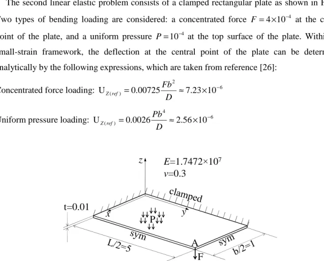
3.2 Bending of a clamped rectangular plate
The second linear elastic problem consists of a clamped rectangular plate as shown in Fig. 8. Two types of bending loading are considered: a concentrated force F= ×4 10−4 at the central point of the plate, and a uniform pressure P=10−4 at the top surface of the plate. Within the small-strain framework, the deflection at the central point of the plate can be determined analytically by the following expressions, which are taken from reference [26]:
Concentrated force loading: 6
2 10 23 7 00725 0 U ( ) = . ≈ . × − D Fb ref Z
Uniform pressure loading: 6
4 10 56 2 0026 0 U ( ) = . ≈ . × − D Pb ref Z
A
z
x
y
F
P
E=1.7472×10
7v=0.3
t=0.01
Fig. 8. Geometry, material properties, and boundary conditions for the clamped rectangular plate.
Owing to the symmetry, only one quarter of the plate is analyzed using the SHB15 and SHB20 elements. The convergence results in terms of normalized deflections at the central point of the plate (point A in Fig. 8), corresponding to both types of loading, are reported in Tables 2 and 3. One can observe that, for this linear elastic test problem, the SHB20 solid‒shell element has a convergence rate similar to that of the ABAQUS shell element S8R, for both considered types of loading, while the convergence of the ABAQUS solid element C3D20 is much slower. For the SHB15 prismatic solid‒shell element, the convergence is slightly slower than that of the ABAQUS triangular shell element STRI65, but faster than that of the ABAQUS prismatic solid element C3D15.
21
Table 2
Normalized deflection at point A: case of concentrated force. Number of
elements
STRI65 C3D15 SHB15 Number of
elements
S8R C3D20 SHB20
UZ/UZ(ref) UZ/UZ(ref) UZ/UZ(ref) UZ/UZ(ref) UZ/UZ(ref) UZ/UZ(ref)
(5×1×2)×1 0.1834 0.0614 0.1845 5×1×1 0.9526 0.0023 0. 9510
(10×2×2)×1 0.8639 0.4618 0.6536 10×2×1 0.8163 0.3956 0. 8017
(20×4×2)×1 0.9934 0.8139 0.9089 20×4×1 0.9905 0.8643 0.9890
(50×10×2)×1 1.0037 0.9743 0.9916 50×10×1 1.0019 0.9755 1.0018
Table 3
Normalized deflection at point A: case of uniform pressure. Number of
elements
STRI65 C3D15 SHB15 Number of
elements
S8R C3D20 SHB20
UZ/UZ(ref) UZ/UZ(ref) UZ/UZ(ref) UZ/UZ(ref) UZ/UZ(ref) UZ/UZ(ref)
(5×1×2)×1 0.3177 0.0149 0.0055 5×1×1 1.0208 0.0018 1.0201
(10×2×2)×1 1.0102 0.5747 0.7762 10×2×1 1.0255 0.6960 1.0289
(20×4×2)×1 1.0248 0.9233 0.9667 20×4×1 1.0176 0.9046 1.0176
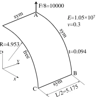
3.3 Pull-out of an open-ended cylindrical shell
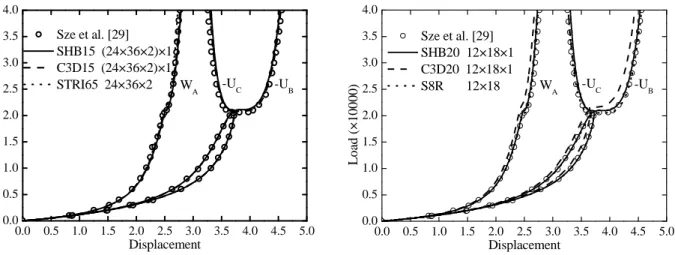
In this test problem, and some others that follow, the performance of the SHB elements will be evaluated in the framework of geometric nonlinearities (i.e., large displacements and rotations). The first test in this category consists of a free elastic open-ended cylindrical shell, which is pulled out by two opposite radial forces as illustrated in Fig. 9. This benchmark test has been studied by several authors (see, e.g., [14, 27‒29]), due to its particular boundary conditions involving very large rotations. Considering the problem symmetry, only one eighth of the cylindrical shell is modeled, as shown in Fig. 9. The load‒displacement curves at point A in the
22
z-direction and at points B and C in the x-direction, which are obtained with the SHB elements,
are compared in Fig. 10 with those given by ABAQUS elements as well as with the reference solution taken from Sze et al. [29]. The shape of the load‒displacement curves reveals that the solution exhibits two main stages: the first stage is governed by bending effects, which is characterized by large displacements and rotations, while the second stage is dominated by membrane effects. The transition between the two stages is marked by a snap-through point at a critical force value of 22×103, which is characterized by a reversal of displacement of point C in the load‒displacement curve. The load‒displacement curves obtained with the SHB elements are in excellent agreement with the reference solution as well as with those given by ABAQUS elements. However, the C3D20 ABAQUS element requires finer meshes in order to obtain an accurate solution for this severe benchmark test.
z y x F/8=10000 A B C R=4.953 t=0.094 E=1.05×10⁷ v=0.3
Fig. 9. Geometry, elastic properties, and boundary conditions for the open-ended cylindrical shell subjected to radial pulling forces.
23 0.0 0.5 1.0 1.5 2.0 2.5 3.0 3.5 4.0 4.5 5.0 0.0 0.5 1.0 1.5 2.0 2.5 3.0 3.5 4.0 WA -UC L o ad ( × 1 0 0 0 0 ) Displacement Sze et al. [29] SHB15 (24×36×2)×1 C3D15 (24×36×2)×1 STRI65 24×36×2 -UB 0.0 0.5 1.0 1.5 2.0 2.5 3.0 3.5 4.0 4.5 5.0 0.0 0.5 1.0 1.5 2.0 2.5 3.0 3.5 4.0 WA -UC L o ad ( × 1 0 0 0 0 ) Displacement Sze et al. [29] SHB20 12×18×1 C3D20 12×18×1 S8R 12×18 -UB
(a) triangular shell / prismatic elements (b) quadrilateral shell / hexahedral elements Fig. 10. Load‒displacement curves for the open-ended cylindrical shell subjected to radial pulling
forces.
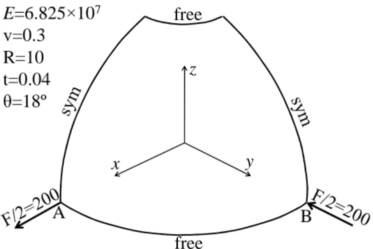
3.4 Hemispherical shell with a hole
Figure 11 illustrates a free hemispherical shell with an 18º circular hole at its pole (see Park et al. [30], Sze et al. [31]). The shell is loaded by a pair of alternating forces at 90° intervals. Owing to the symmetry of the problem, only one quarter of the model is discretized. The simulation results obtained with the SHB elements, in terms of load‒displacement curves at the load points A and B, are compared in Fig. 12 with those given by ABAQUS elements as well as with the reference solutions given by Park et al. [30] and Sze et al. [31]. It can be seen once again that the SHB elements perform very well with respect to the reference solutions, which is also the case for ABAQUS prismatic and shell elements. However, as pointed out in the previous nonlinear benchmark problem, a finer mesh is required for the ABAQUS quadratic solid element C3D20, in order to obtain an accurate solution.
24 free free A B z x y E=6.825×10⁷ v=0.3 R=10 t=0.04 θ=18º
Fig. 11. Geometry, elastic properties, and boundary conditions for the hemispherical shell subjected to alternating radial forces.
0 1 2 3 4 5 6 7 8 9 10 11 0.0 0.5 1.0 1.5 2.0 2.5 3.0 3.5 4.0 L o ad ( × 1 0 0 )
Radial displacements at points A and B Park et al. [30] Sze et al. [31] SHB15 (48×48×2)×1 C3D15 (48×48×2)×1 STRI65 48×48×2 -VB UA 0 1 2 3 4 5 6 7 8 9 10 0.0 0.5 1.0 1.5 2.0 2.5 3.0 3.5 4.0 L o ad ( × 1 0 0 )
Radial displacements at points A and B Park et al. [30] Sze et al. [31] SHB20 12×12×1 C3D20 12×12×1 S8R 12×12 -VB UA
(a) triangular shell / prismatic elements (b) quadrilateral shell / hexahedral elements Fig. 12. Load‒displacement curves at points A and B for the hemispherical shell subjected to
alternating radial forces.
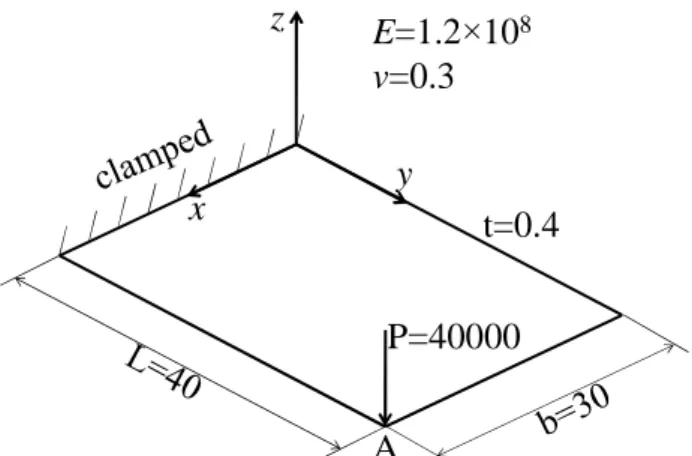
3.5 Cantilever plate subjected to a concentrated force
An elastic cantilever plate with a concentrated force at one corner, as proposed by Hsiao [32], is considered here. The geometric dimensions, elastic properties, and boundary conditions of the problem are all summarized in Fig. 13. Figure 14 reports the load‒displacement curves at the corner point A, in the x, y, and z directions (see Fig. 13). In this Fig. 14, the results obtained with the SHB elements are compared with those given by ABAQUS quadratic solid and shell elements,
25
on the one hand, and with the reference solutions given by Hsiao [32] and Barut et al. [33], on the other hand. These comparisons reveal that the results given by the SHB elements are in very good agreement with the reference solutions, which is also the case with the ABAQUS quadratic shell elements STRI65 and S8R and the ABAQUS prismatic solid element C3D15. However, adopting the same coarse mesh as that used for the SHB20 and S8R elements (i.e., 4×3×1 elements), the solution given by the ABAQUS solid element C3D20 falls far from the reference solution, which confirms once again the need for resorting to much finer meshes to achieve an accurate solution.
z y x A P=40000 t=0.4 E=1.2×10⁸ v=0.3
Fig. 13. Geometry, elastic properties, and boundary conditions for the cantilever plate.
0 5 10 15 20 25 30 35 0 5 10 15 20 25 30 35 40 UA -VA L o ad ( × 1 0 0 0 ) Displacement Hsiao [32] Barut et al. [33] SHB15 (16×12×2)×1 C3D15 (16×12×2)×1 STRI65 16×12×2 -WA 0 5 10 15 20 25 30 0 5 10 15 20 25 30 35 40 UA -VA L o ad ( × 1 0 0 0 ) Displacement Hsiao [32] Barut et al. [33] SHB20 4×3×1 C3D20 4×3×1 S8R 4×3 -WA
(a) triangular shell / prismatic elements (b) quadrilateral shell / hexahedral elements Fig. 14. Load‒displacement curves for the cantilever plate under a concentrated force.
26
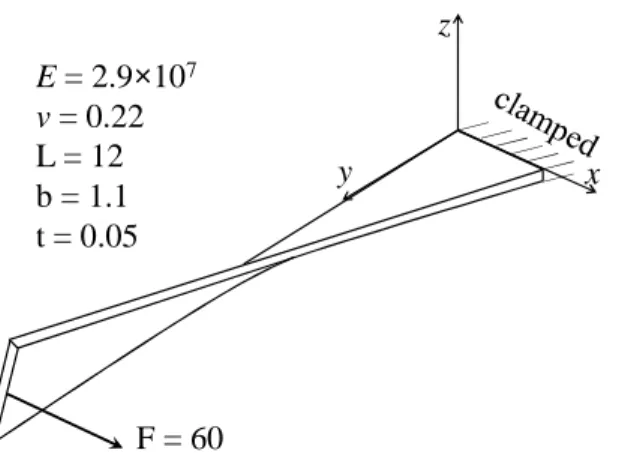
3.6 Bending of a clamped twisted beam
A clamped twisted beam under out-of-plane loading is analyzed in this section, which is considered as a severe nonlinear benchmark test investigated by a number of authors in the literature (see, e.g., [12, 34, 35]). All geometric dimensions and material properties for this twisted beam problem are specified in Fig. 15. The load‒displacement curves at the loading point in the x, y, and z directions are reported in Fig. 16. In this Fig. 16, the results obtained with the SHB elements are compared with those given by ABAQUS quadratic solid and shell elements, on the one hand, and with the reference solution given by Mostafa et al. [35], on the other hand. This comparison shows that the results obtained with the SHB elements are in excellent agreement with the reference solution as well as with that given by the ABAQUS quadrilateral shell element S8R. However, taking the same mesh as that used for the SHB15 element, the ABAQUS triangular shell element STRI65 failed to converge in this nonlinear benchmark test, while the C3D15 element provides less accurate results, which reveals the need for a finer mesh. The latter observation is far more critical for the C3D20 element, which provides once again the farthest results with respect to the reference solution.
x z y F = 60 E = 2.9×10⁷ v = 0.22 L = 12 b = 1.1 t = 0.05
Fig. 15. Geometry, elastic properties, and boundary conditions for the twisted beam subjected to out-of-plane loading.
27 0 1 2 3 4 5 6 7 8 0 10 20 30 40 50 60 L o ad ( N ) Displacement (mm) Mostafa et al. [35] SHB15 (36×6×2)×1 C3D15 (36×6×2)×1 -UZ UX -UY 0 1 2 3 4 5 6 7 8 0 10 20 30 40 50 60 L o ad ( N ) Displacement (mm) Mostafa et al. [35] SHB20 10×2×1 C3D20 10×2×1 S8R 10×2 -UZ UX -UY
(a) triangular shell / prismatic elements (b) quadrilateral shell / hexahedral elements Fig. 16. Load‒displacement curves for the clamped twisted beam subjected to out-of-plane
loading.
3.7 Bending of a clamped curved beam
Bending of a curved beam, as illustrated in Fig. 17, is a typical nonlinear benchmark test for beam structures, in which various deformation modes (e.g., tension, bending, shear) are involved (see Smoleński [34]). The three-dimensional displacement at the loading point is investigated using the proposed SHB elements and ABAQUS quadratic elements. The corresponding load−displacement curves are reported in Fig. 18 along with the reference solution given by Smoleński [34]. As can be seen in Fig. 18, the results obtained with the SHB elements are in excellent agreement with the reference solution as well as with those given by ABAQUS quadratic elements, except for the ABAQUS solid element C3D20. For the latter, the results yielded by a coarse mesh (see Fig. 18 (b)) are far from the reference solution, which reveals that the C3D20 quadratic solid element requires much finer meshes to achieve an accurate solution for this nonlinear test problem.
28 E = 1×10⁷ v = 0. θ = 45º clamped F z x y b = t =1
Fig. 17. Geometry, elastic properties, and boundary conditions for the curved beam.
0 10 20 30 40 50 60 0 100 200 300 400 500 600 L o ad ( N ) Displacement (mm) Smoleński [34] SHB15 (16×2)×1 C3D15 (16×2)×1 STRI65 16×2 UZ UX UY 0 10 20 30 40 50 60 0 100 200 300 400 500 600 L o ad ( N ) Displacement (mm) Smoleński [34] SHB20 4×1×1 C3D20 4×1×1 S8R 4×1 UZ UX UY
(a) triangular shell / prismatic elements (b) quadrilateral shell / hexahedral elements Fig. 18. Load‒displacement curves for the curved beam under a concentrated force.
3.8 Inflation of an elastic‒perfectly-plastic square plate
In this test, the inflation of a simply supported square plate, as illustrated in Fig. 19, is considered to evaluate the performance of the proposed SHB elements in the framework of combined geometric and material nonlinearities (i.e., large strains and plastic behavior). The square plate is simply supported at its four edges, and subjected to uniform pressure loading
0.6
P= . The material parameters of the plate corresponding to elastic‒perfectly-plastic behavior are summarized in Fig. 19 (see [36‒38]). Note that for this nonlinear test, which involves large plastic strains, three integration points through the thickness are required to obtain accurate solutions. Owing to the symmetry of the problem, only one quarter of the square plate is discretized.
29 z y x A P=0.6 t=2.54 E=6.9×10⁴ v=0.3 σ0=248
Fig. 19. Geometry, material properties, and boundary conditions for the simply supported square plate subjected to a uniform pressure.
With the increase in the applied pressure, the square plate undergoes a pillow-type deformation mode, as displayed in Fig. 20, where the plastic zones are mainly localized in the four corners. The simulated pressure‒displacement curves at the center of the plate are depicted in Fig. 21. It can be seen that the results obtained with the SHB elements are in good agreement with the reference solutions taken from Betsch and Stein [36] and Fontes Valente et al. [37] as well as with those given by ABAQUS quadratic elements, except for the C3D20 solid element and the STRI65 shell element. The latter ABAQUS elements provide results that slightly deviate from the reference solutions (see Fig. 21).
(a) SHB15 elements (b) SHB20 elements Fig. 20. Final deformed shape for the square plate under uniform pressure.
30 0 10 20 30 40 50 60 70 80 90 100 0.0 0.1 0.2 0.3 0.4 0.5 0.6 P re ss u re
Displacement at the plate center Betsch and Stein [36]
Fontes Valente et al. [37] SHB15 (24×24×2)×1 C3D15 (24×24×2)×1 STRI65 24×24×2 0 10 20 30 40 50 60 70 80 90 100 0.0 0.1 0.2 0.3 0.4 0.5 0.6 P re ss u re
Displacement at the plate center Betsch and Stein [36]
Fontes Valente et al. [37] SHB20 10×10×1 C3D20 10×10×1 S8R 10×10
(a) triangular shell / prismatic elements (b) quadrilateral shell / hexahedral elements Fig. 21. Load‒displacement curves at the center point of the plate.
3.9 Pinched cylinder with rigid end diaphragms
The second elasto-plastic test consists of a cylinder subjected to two opposite radial forces at its middle and bounded by rigid diaphragms on its ends. This popular benchmark problem has been considered by a number of authors (see, e.g., [37, 39‒41]) to assess the performance of finite elements in large plastic strains. The geometric dimensions, material properties, and boundary conditions of the pinched cylinder are all summarized in Fig. 22. In conjunction with the elasto-plastic material behavior, a linear isotropic hardening law is considered. Owing to the symmetry, only one eighth of the cylinder is modeled.
31 z y x F A t = 3 E = 3000 v = 0.3 σ0 = 24.3 Hiso= 300
Fig. 22. Geometry, material properties, and boundary conditions for the pinched cylinder.
Figure 23 illustrates the final deformed shape of the pinched cylinder, as obtained with the SHB elements. The simulated force−displacement curves at the loading point A (as denoted in Fig. 22) are reported in Fig. 24 along with the reference solutions taken from Wriggers et al. [39], Eberlein and Wriggers [40] and Hauptmann et al. [41]. It can be seen that the results obtained with the SHB elements are in good agreement with the reference solutions along the entire loading history, which is also the case with the ABAQUS prismatic solid element C3D15 and the ABAQUS shell elements STRI65 and S8R. For the C3D20 quadratic solid element, however, the force−displacement response is well predicted during the elastic stage of loading (up to displacement of 100 mm), while the simulated response is overestimated at larger plastic strains (up to 20 % with respect to the reference solutions).
(a) SHB15 elements (b) SHB20 elements Fig. 23. Final deformed shape for the pinched cylinder problem.
32 0 50 100 150 200 250 0 500 1000 1500 2000 2500 3000 F o rc e Displacement Wriggers et al. [39] Eberlein and Wriggers [40] Hauptmann et al. [41] SHB15 (20×20×2)×1 C3D15 (20×20×2)×1 STRI65 20×20×2 0 50 100 150 200 250 0 500 1000 1500 2000 2500 3000 F o rc e Displacement Wriggers et al. [39] Eberlein and Wriggers [40] Hauptmann et al. [41] SHB20 16×16×1 C3D20 16×16×1 S8R 16×16×1
(a) triangular shell / prismatic elements (b) quadrilateral shell / hexahedral elements Fig. 24. Force‒displacement curves at the loading point for the pinched cylinder.
4 Simulation of sheet metal forming processes
This section is dedicated to the validation of the proposed SHB elements in the context of sheet metal forming. To this end, a set of selective benchmark problems are simulated with the SHB elements, which consist of three well-known deep drawing tests as well as an incremental forming process. Despite the strong and coupled nonlinearities involved in such applications (i.e., geometric and material nonlinearities as well as contact), only a single element layer, with three through-thickness integration points, is consistently considered throughout this section, for all meshes consisting of SHB elements. The simulation results are compared both with those given by ABAQUS elements and with experiment measurements taken from the literature.
4.1 Springback simulation of U-shape deep drawing
The springback simulation of the U-shape deep drawing process has been proposed as a benchmark test by the sheet metal forming community in the NUMISHEETʼ93 conference [42]. The schematic view of the setup and its geometric dimensions are described in Fig. 25. All details regarding the simulation process can be found in the related literature (see, e.g., [16, 43‒45]). This deep drawing process is divided into two steps: the forming step, followed by the springback step. During the first step, the U-shape is formed until the maximum punch stroke of 70 mm is
33
reached under a holding force of 2.45 kN (see Fig. 26 (a)). Then, the springback stage of the sheet takes place by removing the holding force and all contact between the sheet and the tools (see Fig. 26 (b)).
6
55
55
50
6
R5
R5
52
R5
1
7
0
punch
holder
holder
die
die
blank
y
x
Fig. 25. Setup of the U-bending tools.
(a) end of forming step (b) after springback
Fig. 26. Illustration of the deformed sheet, in the U-shape deep drawing test, at (a) the end of forming step, and (b) after springback.
Both an aluminum-alloy sheet and a steel sheet are considered in this study. The initial dimensions of the aluminum sheet are 350 mm × 35 mm × 0.81 mm, with a friction coefficient between the tools and the blank equal to 0.162, while the initial dimensions of the steel sheet are 350 mm × 35 mm × 0.78 mm, with a friction coefficient equal to 0.144. The elasto-plastic
34
parameters associated with both materials are summarized in Table 4, in which the following Swift law has been considered to describe isotropic hardening
0
( eqp)n
Y =k ε ε+ , (26)
where εeqp is the equivalent plastic strain (see the plastic yield function defined in Eq. (20)).
Table 4
Elastic properties and Swift’s isotropic hardening parameters.
Material E (MPa) ν ε0 k (MPa) n
Aluminum 71, 000 0.33 0.01658 576.79 0.3593
Steel 206, 000 0.3 0.007117 565.32 0.2589
The anisotropic plastic behavior of the materials is taken into account by considering the Hill [25] quadratic yield criterion. The Lankford coefficients associated with both studied materials are listed in Table 5.
Table 5
Lankford’s coefficients for both studied materials.
Material r0 r45 r90
Aluminum 0.71 0.58 0.70
Steel 1.79 1.51 2.27
Considering the symmetry of the problem, only one quarter of the blank is analyzed. The latter is discretized by (100×5×2)×1 triangular shell or prismatic elements and 100×5×1 hexahedral elements, respectively (the mesh nomenclature is the same as that used in Section 3). As stated before, only three integration points through the thickness are considered in the simulations using the SHB and ABAQUS elements. Note that the simulations with the ABAQUS quadratic shell element S8R failed to converge for both studied materials, which clearly emphasizes the
35
limitations of this shell element in handling double-sided contact in sheet metal forming processes.
To quantify the amount of springback for the blank after the forming stage, the angles around the punch radius and the die radius (θ1 and θ2, respectively, in Fig. 27) are investigated. The simulation results obtained with the SHB elements are compared in Tables 6 and 7 with those given by ABAQUS elements as well as with experimental measurements and numerical solutions available in the literature. On the whole, the angles after springback predicted with the SHB elements are in good agreement with those given by ABAQUS elements, and lie in the intervals defined by the reference results. These results demonstrate the good capabilities of the SHB elements in modeling sheet metal forming processes, where various nonlinearities (geometric, material, and double-sided contact) enter into play, while using only a single element layer with few through-thickness integration points.
A 15 O x y B D E F
36
Table 6
Springback angles θ1 and θ2 for the aluminum material.
Material Angle (°) Experiment* Simulation* STRI65 C3D15 SHB15 C3D20 SHB20
Aluminum 1
θ 101.5º~116.0º 62.0º~134.0º 107.28º 108.87º 102.72º 106.03º 104.13º
2
θ 68.5º~77.5º 63.0º~91.0º 69.85º 69.67º 70.74º 70.74º 74.53º
* Note: The experimental and simulated intervals are given in Flores [16].
Table 7
Springback angles θ1 and θ2 for the steel material.
Material Angle (°) Reference 2* Reference 3* STRI65 C3D15 SHB15 C3D20 SHB20
Steel
1
θ 101.06º 100.82º 97.94º 99.67º 99.37º 97.03º 98.32º
2
θ 79.99º 80.45º 80.10º 80.27º 81.05º 82.33º 82.52º
* Note: Reference 2 corresponds to Dvorkin and Bathe [45], while reference 3 refers to Park and Oh [43].
4.2 Single point incremental sheet metal forming
For the past two decades, the incremental forming technology has attracted much attention due to its advantages in terms of economical operability. Single Point Incremental Forming (SPIF) has become a typical test in the context of incremental forming process (see, e.g., Bouffioux et al., [46], Sena et al. [47]). As illustrated in Fig. 28, a clamped square sheet is gradually deformed in its central area by applying a spherical punch with a radius of 5 mm following a preset path. The punch is initially set to be tangent to the sheet surface, and located 41 mm away from one side of the sheet. The whole forming process consists in the following five steps: 1) the punch indents the sheet with 5 mm depth along the y-direction; 2) the punch moves at the same depth following a line of 100 mm along the x-direction; 3) the punch indents a second time the sheet up to a depth of 10 mm; 4) the punch moves back, at the same new depth, following a line of 100 mm along
37
the x-direction; 5) and finally an unloading step takes place, with the punch returning back to its initial position.
1.5 mm
5 mm
5 mm 100 mm
punch displacement path y x z x y punch blank
Fig. 28. Description of the single point incremental forming test.
The material used for the simulations is an aluminum alloy AA3103-O (see Bouffioux et al. [46]). The associated elasto-plastic material parameters are summarized in Table 8, according to the Swift isotropic hardening law (see Eq. (26)).
Table 8
Material parameters for the AA3103-O aluminum alloy.
Material E (MPa) ν ε0 k (MPa) n
AA3103-O 72, 600 0.36 0.00057 180 0.229
The contact conditions between the punch and the sheet are assumed frictionless. Because the sheet is deformed mainly in the central area, only one half of the model is meshed with (60×15×2)×1 quadratic elements, in the case of prismatic elements, and 60×15×1 quadratic elements, in the case of hexahedral elements (again, the mesh nomenclature is the same as that used in Section 3). The obtained results in terms of punch force‒punch displacement correspond to converged solutions using only a single element layer with three through-thickness integration