2
Remerciements:
Tout d’abord, je me dois de remercier Jean Clobert qui a accepté de m’accueillir à Moulis et qui m’a fait confiance pour réaliser cette thèse.
Un grand merci aussi à Alexis Chaine dont le soutien linguistique et statistique m’a été d’une grande aide.
Merci à la multitude de stagiaires qui ont eu le courage de travailler avec moi sur des projets parfois délicats et en particulier Elvire Bestion qui a grandement participé aux phases initiales du développement de MetaConnec.
Un grand merci à Don M iles sans qui le terrain à Villefort n’aurait pas été si plaisant.
Et enfin un immense merci à Catherine qui m’a soutenu pendant toutes ces années de thèse et m’a permis de terminer malgré le lancement de TerrOïko.
3
Summary/Sommaire:
ABSTRACT:...8
RESUME :...8
INTRODUCTION ...9
I. METACONNECT (ADAPTED FROM MOULHERAT ET AL. SUBMITTED-A)... 24
Model structure ... 25
1 Landscape...26
2 Demography ...26
3 Genetic...29
Model outputs ... 29
Population Viability Analysis... 30
Validation of the mating system toolbox... 32
Validation of the genetic module... 33
MODEL SENSITIVITY: ... 35
Mating system... 35
Landscape resolution, dispersal rule and life strategy impact the outcome linked to dispersal... 35
1 Sensitivity of trajectories to landscape resolution...39
2 Sensitivity on colonization time...41
3 Sensitivity on dispersal ...46
4 Conclusion on the sensitivity to landscape resolution...50
MODEL LIMITATIONS: ... 51
MODEL APPLICATION AND PERSPECTIVE ... 52
II. METACONNECT IN EVOLUTIONARY BIOLOGY: WHAT GENETIC MECHANISMS UNDERLYING MATING STRATEGY EXPRESSION MAINTAIN TRIMORPHISM IN A ROCK-PAPER-SCISSORS GAME? (MOULHERAT ET AL. SUBMITTED-B)... 54
THEORETICAL CONTEXT ... 54
TOOLBOX IMPLEMENTATION ... 59
Male reproductive strategy phenotype and the RPS game... 60
Female reproductive investment as gradient of r-K strategies ... 61
Cost of heterozygosity... 61
RUNNING THE MODEL... 62
Nomenclature and MetaConnect set up... 62
Model scenarios... 64
MAINTENANCE CONDITIONS OF TRIMORPHISM IN THE RPS GAME CONTEXT... 64
RPS GAME FUNCTIONING: DISENTANGLING RPS GAME STRUCTURING FROM DEMOGRAPHIC STRUCTURING OF MORPH FREQUENCIES ... 69
RPS GAME IN UTA STANSBURIANA... 73
CHAPTER CONCLUSION... 75
III. METACONNECT IN CONSERVATION BIOLOGY: CORRIDOR FUNCTIONALITY FOR DRAGONFLIES AND BUTTERFLIES WITHIN THE MONTSELGUES (ARDECHE, FRANCE) BOG NETWORK ... 77
STUDY CONTEXT ... 77
Orthetrum coerulescens functional connectivity (Moulherat 2013b; Moulherat et al. in prep) ... 79
1 Dragonflies 2007 MRR overview and 2011 field work design ...79
MRR survey results ... 81
4
3 MRR analysis...81
a. Meteorological covariates selection ...81
b. Multistate model analysis of Orthetrum coerulescens within the Montselgues’ bog network ...83
c. POPAN analysis and Orthetrum coerulescens population size...85
4 MRR results...86
Population viability analysis ... 89
Corridor functionality for dragonflies ... 92
PHENGARIS ALCON CONSERVATION PLANNING (ADAPTED FROM CORNUAU AND MOULHERAT 2013;MOULHERAT AND CORNUAU 2013)... 93
Study context and MetaConnect parameterization ... 93
Simulation results... 94
Conservation planning and actions proposal... 95
IV. METACONNECT IN REGULATORY STUDIES: LANDSCAPE POTENTIAL FUNCTIONAL CONNECTIVITY FOR THE NATTERJACK TOAD (EPIDALEA CALAMITA) AND SPATIAL PLANNING (ADAPTED FROM MOULHERAT 2013A; MOULHERAT ET AL. SUBMITTED-A) ... 97
METACONNECT SETTING UP ... 98
CURRENT METAPOPULATION FUNCTI ONING ... 100
EXPECTED CONSEQUENCES OF THE INDUSTRIAL AREA DEVELOPMENT AND OF THE HIGH-SPEED RAILWAY BUILDING... 101
V. METACONNECT SENSITIVE INPUT ACQUISITION (ADAPTED FROM LAGARDE ET AL. 2012; STEVENS ET AL. 2013; MOULHERAT ET AL. 2014; GRIMM ET AL. IN PREP; LEGRAND ET AL. SUBMITTED; TROCHET ET AL. SUBMITTED)... 105
EXPERIMENTALLY ESTIMATED MAXIMUM DISTANCE OF MOVEMENT FOR THE MOORISH TOTRTOISE (TESTUDO GRAECA SOUSSENSIS) ... 105
Maximum distance traveling under physiological constraints... 106
Maximum distance traveling by free ranging individuals... 107
Conclusion ... 110
ESTIMATING MAXIMUM DISTANCE DISPERSAL THROUGH META-ANALYSIS AND DATA BASE DEVELOPMENT ... 111
Theoretical framework ... 111
Models... 111
Applicability ... 113
CONCLUSION ... 114
CONCLUSION - FUTURE OF METACONNECT, TERROÏKO’S ACTIVITY ... 115
REFERENCES:... 116
RELATED PAPERS ... 142
1. METACONNECT, A NEW PLATFORM FOR POPULATION MODELING TO ASSIST DECISION MAKERS IN CONSERVATION AND URBAN PLANNING... 143
APPENDIX A:... 178
2. WHAT GENETIC MECHANISMS UNDERLYING MATING STRATEGY EXPRESSION MAINTAIN TRIMORPHISM IN A ROCK-PAPER -SCISSORS GAME? ... 180
APPENDIX A:... 214
APPENDIX B:... 219
ONLINE APPENDIX C: ... 220
ONLINE APPENDIX D: ... 221
3. BUSHES PROTECT TORTOISES FROM LETHAL OVERHEATING IN ARID AREAS OF MOROCCO ... 225
4. HOW FAR CAN A TORTOISE WALK IN OPEN HABITAT BEFORE OVERHEATING?IMPLICATIONS FOR CONSERVATION... 256
5. RANKING THE ECOLOGICAL CAUSES OF DISPERSAL ... 279
5
SUPPLEMENTARY MATERIAL FOR “DISPERSAL SYNDROMES AND THE USE OF LIFE-HISTORIES TO PREDICT DISPERSAL” BY STEVENS
VM,TROCHET A,BLANCHET S,MOULHERAT S,CLOBERT J&BAGUETTE M ... 332
7. INFERRING VAGILITY FROM MORPHOLOGY AND LIFE-HISTORY TRAITS IN EUROPEAN AMPHIBIANS... 349
APPENDIX S1. ... 377
APPENDIX S2. ... 406
APPENDIX S3. ... 413
8. TRAIT DATABASE OF REPTILE LIFE HISTORIES... 443
RELATED SCALES REPORTS... 466
1. REVIEW MANUSCRIPT ON DISPERSAL TRAITS AND DISTANCES, INCLUDING THE UNDERLYING TRAIT DATABASE (GOTZENBERGER ET AL.2011)W.P.2.1.3,114PP ... 467
2. DEVELOPMENT OF DISPERSAL RESPONSE CATEGORIES UNDER DIFFERENT ECOLOGICAL SCENARIOS (BAGUETTE ET AL.2012A) W.P.2.3.1,127PP ... 470
3. REPPORT ON SCALING PROPERTIES OF DECLINING AND EXPANDING POPULATIONS IN RELATION TO UNDERLYING PRESSURE AND ON AREA REQUIREMENTS FOR VIABLES POPULATIONS (CLOBERT ET AL.2012)W.P.2.3.2,213PP. ... 472
4. REPORT ON SCALLING TRADE-OFFS IN CONSERVATION GOALS AND CROSS-SCALE CONSERVATION PRINCIPLES (GUNTON ET AL. 2013)W.P.2.6.2,37PP ... 481
5. ASSESSMENT OF UNCERTAINTY OF SIMPLE CONNECTIVITY ESTIMATES (BAGUETTE ET AL.2012D)W.P.3.2.2,62PP... 482
6. POPULATION VIABILITY ACROSS SCALES (BAGUETTE ET AL.2012C)W.P.3.2.3,88PP... 483
7. SCALE TOOLS ... 484
6
Figure, table and equation tables/Sommaire des figures,
tableaux et équations :
Figures:
FIGURE 1:... 13 FIGURE 2:... 16 FIGURE 3:... 27 FIGURE 4:... 30 FIGURE 5:... 31 FIGURE 6:... 33 FIGURE 7:... 34 FIGURE 8:... 36 FIGURE 9:... 37 FIGURE 10: ... 39 FIGURE 11: ... 40 FIGURE 12: ... 41 FIGURE 13: ... 42 FIGURE 14: ... 43 FIGURE 15: ... 44 FIGURE 16: ... 47 FIGURE 17: ... 48 FIGURE 18: ... 49 FIGURE 19: ... 59 FIGURE 20: ... 66 FIGURE 21: ... 67 FIGURE 22: ... 69 FIGURE 23: ... 72 FIGURE 24: ... 74 FIGURE 25: ... 78 FIGURE 26: ... 80 FIGURE 27: ... 82 FIGURE 28: ... 83 FIGURE 29: ... 90 FIGURE 30: ... 91 FIGURE 31: ... 92 FIGURE 32: ... 93 FIGURE 33: ... 94 FIGURE 34: ... 95 FIGURE 35: ... 96 FIGURE 36: ... 97 FIGURE 37: ... 98 FIGURE 38: ... 100 FIGURE 40: ... 104 FIGURE 41: ... 106 FIGURE 42: ... 107 FIGURE 43: ... 109 FIGURE 44: ... 112 FIGURE 45: ... 1137
Tables/Tableaux :
TABLE I: ... 25 TABLE II: ... 32 TABLE III: ... 63 TABLE IV: ... 68 TABLE V: ... 84 TABLE VI: ... 87 TABLE VII:... 99Equations:
EQUATION 1:... 27 EQUATION 2:... 38 EQUATION 3:... 608
Abstract:
In a context of global change, scientists and policy-makers require tools to address the issue of biodiversity loss. Population viability analysis (PVA) has been the main tool to anderstand and plan for this problem. However, the tools developed during the 90s poorly integrate recent scientific advances in landscape genetics and dispersal. Here, I developed a flexible and modular modelling platform for PVA that addresses many of the limitations of existing software and in this way answer the call made by Evans et al. (2013) for predictive systems ecology models. MetaConnect is an individual-based, process-based and PVA-based modelling platform which could be used as a research or a decision-making tool. In my thesis, I present the modeling base core of MetaConnect and its validation and then present different uses of this plateform in theoretical and applied ecology.
Résumé :
Dans un contexte de changements globaux, les scientifiques et les législateurs requièrent des outils leur permettant de traiter la question de la perte de biodiversité. L’analyse de viabilité de population (PVA) est l’outil principal pour traiter le problème. Cependant, les outils développés dans les années 90 n’intègrent que très peu les récents progrès réalisés en génétic du paysage et sur la compréhension de la dipsersion. Ici, j’ai développé une plateforme de modélisation flexible et modulaire pour réaliser des PVA qui palie à la plupart des limitations des logiciels existants et répondant de ce fait à l’appel fait par Evans et al. (2013) pour développer des modèles prédictifs des systèmes écologiques. MetaConnect est un modèle individu centré, basé sur le déroulement des processus biologiques et principalement basé sur la réalisation d’analyses de viabilités qui peut être utlisé à la fois comme un outil de recherche ou d’aide à la décision. Dans ma thèse, je présente le module central de MetaConnect et sa validation puis présente différentes application de cette plateforme à des fins théoriques et appliquées.
9
Introduction
“Global change refers to planetary-scale changes in the Earth system. The system consists of the land, oceans, atmosphere, poles, life, the planet’s natural cycles and deep Earth processes. These constituent parts influence one another. The Earth system now includes human society, so global change also refers to large-scale changes in society (International Geosphere-Biosphere Programme 2010). More completely, the term “global change” encompasses: population, climate, the economy, resource use, energy development, transport, communication, land use and land cover, urbanization, globalization, atmospheric circulation, ocean circulation, the carbon cycle, the nitrogen cycle, the water cycle and other cycles, sea ice loss, sea-level rise, food webs, biological diversity, pollution, health, over fishing, and more (Steffen et al. 2004).”
The global change concept is recent (1980) and was initially introduced by climatologists who studied if the climate was changing, if this change was predictable and if humans are responsible for such a change (Bolin 1970; Bolin and Bischof 1970; Seiler and Crutzen 1980; Bruhl and Crutzen 1988; Crutzen and Andreae 1990). Human induced climate change as a scientific field has generalized to other scientific fields under the term of “global change”. Global change concerns any change that occurs at the Earth scale under anthropogenic pressure (Wikipedia). The consequences of global change often represent an important direct and indirect risk for public health and/or population safety (Chan et al. 1999; Patz et al. 2000; Gubler et al. 2001; Reiter 2001; Rose et al. 2001; Walther et al. 2002; Townsend et al. 2003; Watson et al. 2005; Reaser et al. 2007; Lenton et al. 2008; Myers and Patz 2009; Nicholls and Cazenave 2010; Mimura 2013). Among the fields encompassed by the term ‘global change’, biodiversity loss is one of the less understood and only has recently been studied (Barbrault 2005; Cardinale et al. 2012). Habitat loss and habitat fragmentation in relation to human activities have become the major threats to biodiversity (IUCN 2013). Over the last centuries, habitat conversion from forest to agriculture has taken over large amounts of lands, leaving species with a shrinking world. This conversion has accelerated over the past decades, with tropical forest being destroyed at annual rates between 1 and 4% of their current areas (Dobson et al. 1997). This habitat destruction is believed to be a major cause of species extinction (Dobson et al. 1997). Habitat fragmentation, another side-effect of human activity, also has profound repercussions on species extinction (Fahrig 2003). Events and international structures like the Earth Summit in Rio de Janeiro (1992) or the Convention on Biological
10
Diversity, encourage awareness in politics and the public about the risks linked to biodiversity loss (Barbrault 2005; Cardinale et al. 2012). Such awareness has led supra-national and national stakeholders to produce legislative and operational tools to face the loss of biodiversity. In the European Union (EU), legislative tools are represented by directives that protect species and their habitat (European directives CEE 1979; 1992), and the operative tools consist on granting biodiversity conservation programs (LIFE, LEADER), and endowed the EU with a reserve site network (Natura 2000 network).
Habitat destruction and fragmentation has consequences from the ecosystem scale (Fahrig 2003; Cardinale et al. 2012; de Mazancourt et al. 2013) to the genetic scale (Ingvarsson 2001; Baguette et al. 2013b). Habitat fragmentation modifies landscape patterns in a four-step process: reduction in habitat ara, increase in number of habitat patches, decrease in size of habitat patches and increase in isolation of patches (Fahrig 2003). This alteration of landscape patterns has diverse effects on population dynamics. As patches become smaller, the size of the population supported decreases; this can increase the stochastic risk of extinction from demographic processes (Legendre et al. 1999; Reed et al. 2002), but also from genetic stochasticity: small populations are more subjected to risks of inbreeding depression (Brook et al. 2002b), loss of genetic diversity and mutation accumulation (Rowe and Beebee 2003). Moreover, by increasing the distances between patches and therefore the risks of dispersal, landscape fragmentation prevents individuals from moving from one population to another. This can hinder the recolonisation of patches where sub-populations have become extinct, leading to stochastic extinction of metapopulations (Fahrig 2003). Furthermore, by reducing gene flow between populations, isolation can lead to genetic structuring of sub-populations and impede genetic rescue of sub-populations with high levels of inbreeding (Ingvarsson 2001; Keller and Waller 2002; Tallmon et al. 2004).
To assist policy makers and landscape planners, ecologist have developed models in order to rationalize conservation planning by conducting predictive studies following three main axes (Hanski and Gilpin 1997):
1. species survival: this approach consists of evaluating the extinction or quasi-extinction probability for a given species. The population viability analysis (PVA) is focused on a species’ population dynamic and aims at estimating whether a species will survive in a given population or landscape (Lacy 1993; Hamilton and Moller 1995; Southgate and Possingham 1995; Brook et al.
11
1997; Beissinger and Westphal 1998; Letcher et al. 1998; Brook et al. 1999; Legendre et al. 1999; Scheller and Mladenoff 2004; Schtickzelle and Baguette 2004). This approach usually devotes little attention to the possible genetic complications that can occur with increasing inbreeding (Brook et al. 2002b) or linked to altered meta-population functioning and its demographic and genetic consequences (but see Lindenmayer et al. 1995; Schtickzelle and Baguette 2004).
2. population genetic structuring: PVA based on genetic viability assumes that inbreeding is deleterious to the individuals and must be avoided (Lande 1995; Grimm et al. 2004; Tallmon et al. 2004; Landguth and Cushman 2010). Indeed, increasing inbreeding is assumed to decrease population adaptability rendering the populations more sensitive to diseases and variations in their environments (Frankham 1998; Reed et al. 2002; Frankham 2005). Theoretical studies show that inbreeding may play a major role in species extinction (Lande 1995). However, the analysis of field data has shown that even though inbreeding plays a role in population viability, this role seems to be minor for most (non-island) populations (Frankham 2005; Pertoldi et al. 2007; Radwan et al. 2010). Indeed, the impact of inbreeding may occur at a long temporal scale (Keller and Waller 2002; Robert et al. 2004; Frankham 2005) and the impact on the immune system and its link to population extinctions remains uncertain (Frankham 2005; Radwan et al. 2010).
3. metapopulation functioning: this axis of PVA development is focused on the fluxes of individuals between patches of a meta-population. This axis takes care of the fact that in a given landscape, some suitable habitat may be sometimes empty of individuals (Hanski and Gilpin 1997). Based on a PVA focused on a single patch approach, this means that the population is extinct. However, individuals coming from other patches near by may colonize or reinforce populations of empty or nearly empty patches (Doak and Mills 1994). Similarly, genetic variability in a single patch may be maintained by individual flow coming from the surrounding patches (Hastings and Harrison 1994; Tallmon et al. 2004). Such a system may lead to cases where persistence of a species cannot be insured by a single patch but requires by a patch network (Hanski and Gilpin 1997; Pritchard et al. 2000).
12
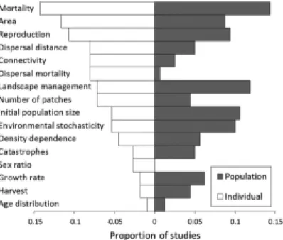
During the 90s, decision making tools were developed on the basis of PVA models mostly build with matrix based models (Box A) (Caswell 2001; Pe'er et al. 2013). Several software packages like ALEX, RAM AS, GAPPS, INM AT, ULM or VORTEX were developed as generic tools to perform PVA analysis (Harris et al. 1987; Akçakaya and Ferson 1990; Lacy 1993; Akçakaya 1994; Mills and Smouse 1994; Legendre and Clobert 1995; Akçakaya et al. 2003) and used by the IUCN experts to determine species’ threat level (Brook et al. 1997). In the 90s matrix based models were preferred to more complex and realistic individual processes based models due to the computational requirement of such models (Hanski and Gilpin 1997), although a few relational generic models were developed (ULM, VORTEX) (Box A). At the time of very limited computational power, matrix based models permitted to work at the population level using appropriate and powerful mathematical tools (Leslie 1945; Ferriere et al. 1996; Caswell 2001). Nowadays, even though matrix based models are still a very widespread tool, the development of computational power allows building more realistic models based on individual characteristics and behavior (individual based model: IBM) driven by biological processes (process based model) that can impact the global population/meta-population persistence and evolution (Doebeli and Koella 1994; Lindstrom and Kokko 1998; Doebeli and de Jong 1999; Hochberg et al. 2003; Sinervo and Clobert 2003; Sinervo and Calsbeek 2006; Cote and Clobert 2007; Duckworth 2009). The ability of integrating different components of individuals characteristics (i.e. the use of IBM) to perform PVA (Pe'er et al. 2013) permit to better understand how individual characteristics and behavior affect a species persistence and to elucidate some links between individual life history traits (LHTs) and their impact at the population level (Figure 1) (Travis and Dytham 1999; Travis et al. 1999; DeAngelis and Mooij 2005; Moulherat et al. submitted-b). However, if IBMs have permitted a better understanding of key processes involved in PVAs, they have also led to a high number of models with their specific output and metrics that are usually hard or impossible to compare with other models(DeAngelis and Mooij 2005; Kindlmann and Burel 2008; Pe'er et al. 2013). Such diversity could be a major constraint on the use of IBMs to perform PVAs and integrate the results into conservation planning because:
1. Conservation managers and policy makers have difficulties to find the best model for the question they seek to address (ITTECOP 2013)
2. It is recommended to use PVAs by making output comparison under different scenarios (scenarios of modeling assumptions) rather than absolute results of each independent scenario that may require multiple models with comparable outputs
13
(Brook et al. 1997; Burgman and Possingham 2000; Pe'er et al. 2013). However, usually, model outputs are specific to the software used and few software packages are flexible enough to allow the building of various scenarios (Brook et al. 1997; Grimm et al. 2004; DeAngelis and Mooij 2005; Pe'er et al. 2013).
3. IBMs require highly detailed information and a strong understanding of the model structure, applicability and limits which are often poorly detailed (DeAngelis and Mooij 2005; Grimm et al. 2006; Urban et al. 2009; Pe'er et al. 2013) as well as a solid theoretical background to limit misinterpretations of results (Ferriere et al. 1996; Burgman and Possingham 2000; Caswell 2001; Urban et al. 2009).
Figure 1: The frequency of papers reviewed in the SCALES project that explored the effect of key parameters on viability on the basis of individual-based (white) or population-based (shaded) models (Pe'er et al. 2013).
14
Box A: Matrix based model or relational models
Matrix based models are suitable for any system that can be represented as a graph (sensu Euler 1741 figure X.a) and used in population dynamics to model at the population scale the summary of individual characteristics (Caswell 2001). This approach was initially developed to work on age-structured population to outperform life table analysis (Leslie 1945). This framework permits numerous developments (two sex models, meta-population models … see Caswell 2001 for details and other developments) under an efficient computational environment. This approach is mainly driven by the definition of a transition matrix A that will determine the population structure (N) at + 1 (Leslie 1945; Caswell 2001).
Figure A.1: Two age-class, one sex life-cycle graphs for passerines where is the juvenile survival rate, the subadult survival rate, the adult survival rate, the subadult fecundity, the adult fecundity and the primary female sex-ratio (adapted from Legendre et al. 1999)
However, while any matrix based model can be translated into relation based models; all relation based models are not likely to be translated into matrix based models (Figure A.2). Indeed, all systems cannot be represented as a graph (i.e. mating systems based on individual characteristics, interactions genotype/phenotype …). In that sense, relational models are more flexible by their structure but require more computational power (DeAngelis and Mooij 2005; Pe'er et al. 2013) and many mathematical tools as sensitivity analysis cannot be used (Cross and Beissinger 2001; Naujokaitis-Lewis et al. 2009).
Figure A.2: Flow chart for the individual-based simulation model of a bear population (Wiegand et al. 1999). The flow chart shows each of the events that can happen to a female bear during the yearly step of the model: dispersal, reproduction, survival, and independence (from the mother). Each of these events is governed by one or more rules not shown here (adapted from DeAngelis and Mooij 2005).
Currently many non-generic models are built with a mixture of matrix based and relation based models especially in order to build non-linear and/or time variant A.
15
Currently, IBMs to perform PVAs have limited flexibility that restrains their application to the scientific field in which they were developed (DeAngelis and Mooij 2005) and models that deal with demography have little way of incorporating genetic factors and dispersal behavior into their analysis. Models based on genetic PVAs (e.g. SPLATCHE (Currat et al. 2004), CDPOP (Landguth and Cushman 2010), META-X (Grimm et al. 2004)) assume over-simplified demographic systems (Baguette et al. 2013b; Pe'er et al. 2013). The main goal of my PhD was to develop a generic IBM, that allows an integration of a large array of demographic, genetic and dispersal processes. In this respect, the idea was to develop a core base computational module based on a demographic PVA model where one could develop and plug in modules for genetic system, dispersal, or other features and then output results that contain similar metrics to permit comparisons between models, situations, scenarios, and so on (Figure 2). Since PVA models aims to determine extinction or quasi-extinction probabilities of a population, they have to simulate the population dynamic at a selected time horizon. This means that PVA models are population dynamic models with a specific output concerning extinction probability that can be ignored or removed for other purposes. The objective of this model is to be a modeling platform (MetaConnect) that could satisfy the needs of researchers from different disciplinary fields (conservation biology, landscape ecology, landscape genetic, evolutionary biology…) as well as conservation managers, policy makers and planning managers that also could be upgraded to incorporate new relevant modules and methods. In this respect, I will present in the first chapter the core base modeling structure of MetaConnect. Then the second chapter is devoted to the use of MetaConnect in evolutionary biology. The third chapter deals with the applied use of MetaConnect with respect to conservation programs. The use of MetaConnect in applied regulatory studies is showed in chapter four. The Fith chapter is focused on complementary studies that could allow “feeding” MetaConnect. Indeed, as MetaConnect is an IBM, it requires considerable input data that are mostly easy to obtain through the available literature. However other variables, such as maximum distance dispersal of species, which are known to be a critical to (met-)population dynamics can be explored through model sensitivity. In other words, a small variation of this variable may induce a large change in the simulation outcome (Ruckelshaus et al. 1997; Tischendorf 2001).
16
Figure 2: MetaConnect assemblage. The Figure presents the core based PVA model (Moulherat et al. submitted-a) with examples of additional plugins that increase and complete the core base model flexibility and applicability (Moulherat et al. submitted-a; Moulherat et al. submitted-b). Pre and post-simulation modules will allow using previously developed
17
models such as LANDIS (Scheller and Mladenoff 2004), GRAPHAB (Foltete et al. 2012) or n_w (Gauzens et al. 2013) and an interface to use R (R Development Core Team 2005). *Bio-SUM COSA project submitted to FRB (Fondation pour la Recherche pour la Biodiversité) 2013 grant.
18
« Les changements globaux font références à des modifications systémiques à l’échelle planétaire. Les systèmes généralement considérés sont la vie des terres, des océans, de l’atmosphère, des pôles, mais aussi les cycles naturels planétaires ou les processus de la dynamique du manteau terrestre, ces différents éléments s’influençant les uns les autres. Les systèmes planétaires incluent dorénavant la société humaine. Les changements globaux font donc aussi références aux modifications des modifications sociétales à large échelle (International Geosphere-Biosphere Programme 2010). Plus complètement, le terme « changement global » recouvre les thématiques de : population, climat, économie, gestion des ressources, développement énergétique, transports, communication, utilisation des sols et végétation, urbanisation, globalisation, circulation atmosphérique, circulation des océans, cycle du carbone, cycle de l’azote, cycle de l’eau et autres cycles, disparition des banquises, niveau des mers, chaine alimentaires, diversité biologique, pollution, santé, surpêche, et bien d’autres (Steffen et al. 2004) . » (Wikipedia).
Le concept de changement global est récent (1980) et a initialement été introduit par les climatologistes qui cherchaient à déterminer si le climat changeait, si ces changements étaient prévisibles et si l’Homme avait une responsabilité dans ces changements (Bolin 1970; Bolin and Bischof 1970; Seiler and Crutzen 1980; Bruhl and Crutzen 1988; Crutzen and Andreae 1990). La conception initiale du réchauffement globale d’origine anthropique a de nos jours été transposé à toutes les disciplines scientifiques sous le terme générique de « changement global ». Le terme de changement global, est utilisé pour toute modification d’origine anthropique ayant des répercussions à l’échelle planétaire (Wikipedia). Les conséquences d’un changement global représentent généralement un risque direct ou indirect sur la santé publique et/ou la sécurité des populations humaines (Chan et al. 1999; Patz et al. 2000; Gubler et al. 2001; Reiter 2001; Rose et al. 2001; Walther et al. 2002; Townsend et al. 2003; Watson et al. 2005; Reaser et al. 2007; Lenton et al. 2008; Myers and Patz 2009; Nicholls and Cazenave 2010; Mimura 2013). Parmi les thématiques scientifiques couvertes par le terme de changement global, l’érosion de la biodiversité est l’un des moins bien étudiés et des plus récemment perçu comme une préoccupation majeure (Barbrault 2005; Cardinale et al. 2012). La destruction et la fragmentation des habitats liés à l’activité humaine sont devenues les principales menaces pour la biodiversité (IUCN 2013). Durant les derniers siècles, l’extension des terres agricoles au détriment des espaces forestiers a contraints les espèces dans des espaces de plus en plus restreints. Cette conversion des espaces c’est accélérée au cours des dernières décennies avec notamment une destruction des forêts
19
tropicales à un taux annuel moyen de 1 à 4% de leurs surfaces actuelles (Dobson et al. 1997). La fragmentation des habitats, un autre effet collatéral de l’activité humaine, a aussi des répercussions profondes sur les extinctions d’espèces (Fahrig 2003). Des évènements et des structures internationales tels que le « Earth Summit » à Rio de Janeiro (1992) ou la « Convention on Biological Diversity », participent à la sensibilisation du grand publique et des politiques aux problématiques liées à la perte de biodiversité (Barbrault 2005; Cardinale et al. 2012).Une telles prise de conscience a conduit les parties prenantes nationales et supranationales à se doter d’outils législatifs et opérationnels pour lutter contre l’érosion de la biodiversité. En Europe (EU), les outils législatifs sont représentés par les directives qui protègent directement les espèces et leurs habitats (European directives CEE 1979; 1992), et d’outils opérationnelles consistant à financer des projets de conservation (LIFE, LEADER), et se doter d’un réseau de sites protégés (réseau Natura 2000).
La destruction des habitats et leur fragmentation a des conséquences de l’échelle écosystémique (Fahrig 2003; Cardinale et al. 2012; de Mazancourt et al. 2013) à l’échelle génétique (Ingvarsson 2001; Baguette et al. 2013b). La fragmentation des habitats modifie le facies paysager via un processus en quatre étapes : réduction des surfaces habitables, augmentation du nombre de patches d’habitats, réduction de la taille des patches d’habitat et isolement des patches d’habitat (Fahrig 2003). Cette altération des paternes paysagers a diverses impactes sur les dynamiques populationnelles. Par la réduction des patches, la taille des populations y vivant se réduit ce qui peut conduire à une augmentation du risque d’extinction dues à la stochasticité démographique (Legendre et al. 1999; Reed et al. 2002), mais aussi dues à la stochasticité d’origine génétique : les populations les plus petites sont plus sujettes aux risques liés à la consanguinité (Brook et al. 2002b), la perte de diversité génétique et l’accumulation de mutations délétères (Rowe and Beebee 2003). De plus, en augmentant la distance entre les patches d’habitat, et par là même, la prise de risque pendant la dispersion, la fragmentation des habitats, limite les échanges d’individus entre patches d’habitat. Ceci peut raréfier la recolonisation des patches préalablement éteints augmentant les risques d’extinction stochastique de la metapopulation (Fahrig 2003). Qui plus est, en réduisant le flux d’individus entre les populations, l’isolement génétique peut mener à une structuration génétique qui limitera le potentiel de sauvetage génétique des populations fortement consanguines (Ingvarsson 2001; Keller and Waller 2002; Tallmon et al. 2004).
20
Afin d’assister le législateur et les aménageurs du territoire, les écologues ont développé des modèles visant à rationaliser les programmes de conservation en réalisant des études prospectives suivant trois axes principaux (Hanski and Gilpin 1997):
1. La survie des espèces : cette approche consiste à évaluer la probabilité d’extinction ou de quasi-extinction d’une espèce donnée. L’analyse de viabilité de population (PVA) est focalisée sur la dynamique populationnelle d’une espèce et cherche à prévoir si cette espèce parviendra à se maintenir dans un paysage donné (Lacy 1993; Hamilton and Moller 1995; Southgate and Possingham 1995; Brook et al. 1997; Beissinger and Westphal 1998; Letcher et al. 1998; Brook et al. 1999; Legendre et al. 1999; Scheller and Mladenoff 2004; Schtickzelle and Baguette 2004). Cette approche n’intègre généralement que peu ou pas les complications génétiques pouvant survenir pour des populations de petites tailles avec une forte consanguinité (Brook et al. 2002b) ou le lien avec le fonctionnement de la metapopulation et ses conséquences sur la démographie et la génétique (cependant voir Lindenmayer et al. 1995; Schtickzelle and Baguette 2004).
2. Structuration génétique des populations : les PVA basées sur la viabilité génétique supposent que la consanguinité est délétère pour la survie des individus et doit être évitée (Lande 1995; Grimm et al. 2004; Tallmon et al. 2004; Landguth and Cushman 2010). En effet, il est considéré que l’augmentation de la consanguinité réduit le potentiel adaptatif des populations les rendant plus vulnérable aux épidémies et variations de l’environnement (Frankham 1998; Reed et al. 2002; Frankham 2005). Des études théoriques ont montrées que la consanguinité pouvait jouer un rôle majeur dans l’extinction des espèces (Lande 1995). Cependant, l’analyse de données de terrain a montré que bien que la consanguinité joue un rôle dans la viabilité des populations, celui-ci est mineur dans la plupart des cas (excepté pour les systèmes insulaires) (Frankham 2005; Pertoldi et al. 2007; Radwan et al. 2010). En effet, l’impact de la consanguinité peut n’avoir une échéance qu’à long terme (Keller and Waller 2002; Robert et al. 2004; Frankham 2005) et son impact sur le système immunitaire ses implications sur l’extinction des populations reste incertain (Frankham 2005; Radwan et al. 2010).
21
3. fonctionnement des métapopulations : cet axe de développement des PVA est focalisé sur le flux d’individus entre les patches d’habitat favorable d’une métapopulation. Cet axe est attentif au fait qu’au sein d’un paysage donné, des habitats favorables sont parfois susceptible d’être inhabités (Hanski and Gilpin 1997). Une PVA basée sur une seule population, considèrerait que la population est éteinte. Cependant, des individus venant de patchs proches sont susceptible de coloniser ces patchs pour lesquels la population est éteinte ou de renforcer des populations en quasi extinction (Doak and Mills 1994). De façon similaire, la variabilité génétique peut être maintenue par le flux d’individus venant de patches alentours (Hastings and Harrison 1994; Tallmon et al. 2004). De tels fonctionnement peuvent mener à des cas où la persistance des espèces ne peut être assuré par une seule et unique population mais par un réseau de patch de populations (Hanski and Gilpin 1997; Pritchard et al. 2000).
Au cours des années 90, les outils d’aide à la décision ont été bâtis sur la base de modèle matriciels de PVA (Box A) (Caswell 2001; Pe'er et al. 2013). Des logiciels tels que ALEX, RAM AS, GAPPS, INM AT, ULM ou VORTEX ont été développés comme des outils de PVA génériques (Harris et al. 1987; Akçakaya and Ferson 1990; Lacy 1993; Akçakaya 1994; Mills and Smouse 1994; Legendre and Clobert 1995; Akçakaya et al. 2003) et utilisés par les experts de l’IUCN pour déterminer le statut de protection des espèces (Brook et al. 1997). Dans les années 90, les modèles matriciels étaient préférés à des modèles individu et processus centrés plus réalistes mais plus complexes en raison des limitations technologiques requises par de tels modèles (Hanski and Gilpin 1997) et seuls quelques modèles relationnels ont été développés (ULM, VORTEX) (Box A). A l’époque où la puissance de calcul était très limitée, les modèles matriciels ont permis de travailler à l’échelle populationnelles à l’aide d’outils mathématiques appropriés (Leslie 1945; Ferriere et al. 1996; Caswell 2001). De nos jours, bien que les modèles matriciels soient toujours très utilisés, l’augmentation de la puissance de calcul permet de construire des modèles plus réalistes basés sur les caractéristiques et comportements individuels des espèces (modèles individus centrés : IBM) sous tendus par des processus biologiques identifiés (modèle processus centré) qui peuvent affectés la persistance et l’évolution des populations/métapopulations à l’échelle globales (Doebeli and Koella 1994; Lindstrom and Kokko 1998; Doebeli and de Jong 1999; Hochberg et al. 2003; Sinervo and Clobert 2003; Sinervo and Calsbeek 2006; Cote and Clobert 2007; Duckworth 2009). La capacité d’intégration de différentes caractéristiques individuelles (i.e.
22
l’utilisation d’IBM) pour réaliser des PVA permet de mieux comprendre comment les caractéristiques et comportements individuels affectent la persistance des espèces (Pe'er et al. 2013) et de comprendre les liens existants entre traits d’histoire de vie (LHT) et leurs impacts à l’échelle populationnelle (Figure 1) (Travis and Dytham 1999; Travis et al. 1999; DeAngelis and Mooij 2005; Moulherat et al. submitted-b). Cependant, si les IBM permettent une meilleur compréhension des processus clés impliqués dans les PVA, ils mènent aussi à un nombre considérable de modèles avec leurs sorties et métriques spécifiques qui sont généralement difficiles voire impossible à comparer entre elles (DeAngelis and Mooij 2005; Kindlmann and Burel 2008; Pe'er et al. 2013). Une telle diversité peut être une contrainte à la généralisation des IBM pour réaliser des PVA et intégrer les résultats dans des programmes de conservation. Les raisons en sont :
1. Les gestionnaires de programmes de conservation et les législateurs ont des difficultés à trouver les modèles adaptés à leurs besoins (ITTECOP 2013).
2. Il est recommandé de réaliser des PVA en comparant les résultats issus de différents scenarios (scenarios d’hypothèses de modélisation) plutôt que les résultats absolus d’un unique scenario (Brook et al. 1997; Burgman and Possingham 2000; Pe'er et al. 2013). Cependant, généralement, les sorties de modèles sont spécifique à l’utilité du logiciel et seuls quelques rares logiciels sont suffisamment flexible pour réaliser des scenarios variés (Brook et al. 1997; Grimm et al. 2004; DeAngelis and Mooij 2005; Pe'er et al. 2013).
3. L’utilisation des IBM nécessitent une grande quantité de données détaillées et une solide compréhension de la structure des modèles, de leurs champs d’applications et de leurs limites qui sont généralement peut détaillés (DeAngelis and Mooij 2005; Grimm et al. 2006; Urban et al. 2009; Pe'er et al. 2013) ainsi que de solides bases théoriques pour limiter les interprétations des résultats erronées (Ferriere et al. 1996; Burgman and Possingham 2000; Caswell 2001; Urban et al. 2009).
Actuellement, les IBM existant pour réaliser des PVA ont une flexibilité limitée, ce qui restreint leur utilisation au champ disciplinaire scientifique pour lequel ils ont été conçu (DeAngelis and Mooij 2005) et les modèles traitant des aspects démographiques n’ont que peu de moyens d’intégrations des problématiques génétiques et de dispersion. Les modèles de PVA basés sur la génétique (SPLATCHE (Currat et al. 2004), CDPOP (Landguth and Cushman 2010), META-X (Grimm et al. 2004)) utilisent des présupposés démographiques présentant une simplification excessive (Baguette et al. 2013b; Pe'er et al. 2013). L’objectif
23
principal de ma thèse a été de développer un IBM générique permettant une intégration large des processus démographique, génétique et de dispersion. Pour ce faire, l’idée a été de un corps de logiciel basé capable de réaliser des PVA et de greffer à ce corps des modules de génétique, de dispersion, mais aussi les modules d’analyse des résultats permettant la comparaison entre différents modèles et scenarios de modélisation (Figure 2). Comme les modèles de PVA ont pour objectif de déterminer les probabilités d’extinction ou de quasi extinction à un horizon donné, ils sont basés sur des modèles de dynamique de populations présentant une sortie spécifique permettant de calculer les probabilité d’extinction et qui, de fait peuvent être aisément ignorer ou supprimer pour des objectifs différents. L’objectif de mon modèle est de devenir une plateforme de modélisation (MetaConnect) satisfaisant à la fois les scientifiques de différentes disciplines (biologie de la conservation, écologie du paysage, génétique du paysage, biologie évolutive,…) aussi bien que les gestionnaires d’espaces naturels, les législateurs et les aménageurs du territoire et pouvant être mis à jour pour incorporer de nouveaux modèles et méthodes pertinents. Pour ce faire, je présente ici dans le premier chapitre, le corps de MetaConnect. Par la suite, le second chapitre est dédié à l’utilisation de MetaConnect en biologie évolutive. Le troisième chapitre quant à lui porte sur l’utilisation appliquée sur le terrain de MetaConnect dans des programmes de conservation. L’utilisation de MetaConnect dans les études réglementaire est traité en chapitre quatre. Le cinquième chapitre est focalisé sur des études connexes qui permettent de « nourrir » MetaConnect. En effet, comme MetaConnect est un IBM, il nécessite de nombreuses données d’entré qui peuvent être majoritairement extraites de la littérature mais certaines variables telles que la distance maximum de dispersion des espèces sont reconnues comme critiques au regard de l’analyse de sensibilité et doivent faire l’objet d’une attention particulière. En d’autres termes, une petite variation de cette variable est susceptible d’engendrer des résultats de simulations très différents (Ruckelshaus et al. 1997; Tischendorf 2001).
24
I. MetaConnect
(adapted from Moulherat et al. submitted-a)The core base modeling of MetaConnect is a simple population dynamic model which can be used as a standalone application to perform PVAs. However, if the core base model estimates extinction probabilities, it also simulates the complete population dynamic tagging individuals with genetic tags (neutral alleles such as microsatellites).
Model design
MetaConnect simulates metapopulation dynamics and genetics using the species life cycle and life history traits, the landscape characteristics and their interactions. The simulations allow inferring of local and global extinction probabilities, individual dispersal within the meta-population, local and global genetic diversity and local and global genetic differentiation (from classical Fst analyses or as input files for Structure software (Pritchard et al. 2000)).
MetaConnect is an individual and process-based-model which means that:
(1) all individuals in the model are independent and behave in respect to their phenotype (individual-based model)
(2) patterns emerging in the different outputs of the model are the products of flexible and adjustable rules implemented in the model (process-based-model).
25
Model structure
Table I: Nomenclature of MetaConnect’s main parameters and variables.
Parameters and
variables Description law of random Distribution
variables Demographic characteristics Carrying capacity*
Total com petition coefficient Survival of individual from class i Fecundity
Primary sex ratio
Bernoulli Poisson Bernoulli
Mating system
Mating system Mating system assumptions
Male harem size
Female harem size Poisson Poisson
Genetics
Number of loci Number of alleles per locus
Mutation rate
Dispersal
Dispersal rule Dispersal probability Dispersal algorithm Bernoulli
Initialization and model parameterization
Initial number of individuals
Initial sex-ratio Initial class structure Time steps
Number of landscape random generations
Number of population dynam ic simulations per landscape
* The carrying capacity K is derived from the competition coefficient and the competition assumptions.
26
1 Landscape
The modeling platform MetaConnect requires three layers describing the landscape:
(1) Patches: locales of suitable habitat for the focal species. Each patch is identified by its name and is constituted by all the adjacent cells having the same name.
(2) Carrying capacities: provides the carrying capacity for each cell of the layer. The patch carrying capacity then corresponds to the mean value of its constitutive cell’s carrying capacities.
(3) Costs: provides a coefficient representing preferences for each cell of the map The landscape layers can be imported from GIS software as raster files.
2 Demography
The population dynamics are represented by a succession of individual states linked by transitions. The user can build the species life-cycle by assembling “bubbles” representing the individual state and “arrows” representing transition rules between individual states (Figure 3). The “bubbles” correspond to what we will call “class” along this manuscript and can correspond to age classes or sex or anything that can be defined as a group of individuals with the same demographic characteristics. Density dependence can be a scramble or contest and can be designed as a part of a transition. The mating system can be chosen from monogamy, polygamy, polyandry and/or polygyny (Legendre et al. 1999). The demographic parameters (Table 1) can be patch-specific. Environmental stochasticity has been included as random processes inducing normal variation around the patch’s mean value of demographic parameters. As an example, the fecundity parameter follows a Poisson distribution (demographic stochasticity) with parameter λ equal to the average fecundity ( ↝ ( )). The average fecundity can vary from one patch to another and within simulation time steps following a Gaussian distribution (Table 1).
27
Figure 3: Example of the Legendre et al. (1999) passerine life cycle with two age-classes and two sexes that can be modeled with MetaConnect. On this MetaConnect screenshot, in the A section, “bubbles” correspond to reproductive status of individuals (subadult or adult) and dd is the density-dependent recruitment probability that depends on the competition assumption (contest or scramble competition respectively equations 1a and 1b). The user defines the species life-cycle as a combination of settable “bubbles” (add class) and “arrows” (add transition) (A). The species life history traits are set up in the B section and the run settings are defined in the C section. Then, the MetaConnect workflow (D) and the Leslie matrix (E) are generated automatically. The Leslie matrix and the MetaConnect workflow can be changed by the user which automatically adjusts the life-cycle graph.
Dispersal decision is implemented by setting a proportion of individuals (reproductive and/or non-reproductive) leaving a patch. The density-dependent recruitment probabilities is determined by equation 1 where can be a chosen combination of the number of individuals per class (i.e. .could be the total population or just the reproductive individuals) (Caswell 2001).
Equation 1:
28
If scramble competition: =
Dispersal is age- and sex-dependent, and the process by which individuals disperse can be chosen from three families of movement rules:
1. The first family of dispersal rules does not take account of the preference coefficients. Dispersal between patches is modeled by a probability for an individual to reach another patch. The probability of reaching a patch can be equal between patches, or depend on the Euclidean distance between patch centers, or can be set manually. 2. The second family represents the interaction between individuals and their
environment through the use of preference coefficients. This family comprises the random-walk dispersal rule (RW) and a correlated random-walk rule (CRW). The CRW assumes a degree of directional persistence, (i.e., the movement direction at time t+1 depends on the direction taken at time t) and not solely an environmental based one.
3. The last family of rules assumes that individuals have knowledge of their environment. They are able to reach the other patches by taking the easiest route (Least-Cost-Path, LCP). From a focal patch, the LCP algorithm usually assumes that a single patch can be reached (Botea et al. ; Adriaensen et al. 2003; Pe'er and Kramer-Schadt 2008; Barraquand et al. 2009). Such an assumption is unrealistic, and to relax it we implemented a multiple LCP movement rule, in which we calculated all possible combinations of LCPs between the focal patch and all the other patches (Urban et al. 2009; Foltete et al. 2012). Then, for the reachable patches (i.e. LCP length less than the maximum dispersal distance), the probability to reach a patch is weighted by the LCP length (number of map cells crossed) or cumulative cost (total cost of all map cells crossed). We also adapted the Stochastic Movement Simulator (SMS) (Palmer et al. 2011; Coulon et al. in prep), which relaxes the assumption of omniscience inherent in the LCP approach. With the SMS rule, individuals make movement decisions based on the environment within a limited perceptual range and a tendency to directional persistence similar to that in a CRW. At each movement time step, the SMS algorithm calculates a movement probability for each cell surrounding the individual’s current cell. The calculation process evaluates the displacement cost for each surrounding cell
29
based on the coefficient of rugosity of the cells in the neighborhood and its distance to the current place (see Palmer et al. 2011 for details).
The dispersal event ends when the individual dies or reaches a patch different from his original patch regardless of the arrival patch quality.
3 Genetics
Individuals are genetically tagged using neutral polymorphic loci. The number of loci and number of alleles per locus can be specified by the user. A single mutation rate (probability of creating a new allele without possibility of reverse mutation) implemented in the model allows the production of new alleles at each locus during simulations, and can be specified by the user. Gene transmission is assumed to be Mendeleian and siblings are assumed to have the same father (randomly chosen from the female harem for polyandrous cases).
Model outputs
The model provides many forms of outputs based on focal species life history traits and landscape maps, which are adaptable to various theoretical and applied contexts. The outputs report the results at three levels at a frequency specified by the user, allowing dynamic visualization of the simulations:
1. Demography: the model provides population size that can be split into the different classes implemented in the MetaConnect set up. The model also derives extinction probability, colonization probability and time before extinction and colonization. These indicators are calculated at the local (patch) and global (metapopulation) scales. 2. Dispersal: for each pair of patches, the model provides the number of individuals that
reach a new patch or die during the dispersal process. In addition, maps of cell occupancy are drawn from successful dispersal events (number of individual who visited the map cells during the whole run).
3. Genetics: the model provides the genetic diversity and differentiation (Fst, Fis, Fit, He and Ho) at the local and global scale.
30
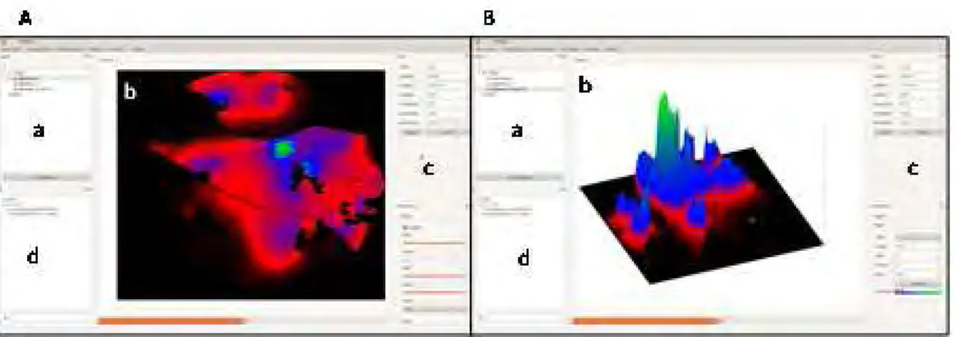
All these results can be directly plotted using the MetaConnect results viewer (Figure 4) or extracted as text files. In addition R (R Development Core Team 2005) has been incorporated to the viewer, which allows direct analysis of the MetaConnect outputs.
Figure 4: Screenshot of an example of MetaConnect results. Data to be displayed or analyzed are selected in the “a” section and displayed in the “b” section in two (A) or three (B) dimensions. Section “c” allows setting of the display options, and the “d” section is an R console to perform simple analysis and plotting of the MetaConnect outputs. An R package and a specific section of MetaConnect are under development for a complete integration of R into MetaConnect.
Model validation:
As suggested by Pe’er et al. (2013), we validated the MetaConnect component by comparing its results when possible with results provided by equivalent analytical models and IBMs. Results from MetaConnect and previous models matched well, and we present here only the most important comparisons that pertain to MetaConnect PVA core modeling, namely the validation of (1) the demographic core modeling, (2) the mating system toolbox and (3) the genetic module.
Population Viability Analysis
Brook et al. (1997) compared the ability of 5 PVA packages (INM AT, GAPPS, RAM AS/age, RAM AS/metapop and VORTEX which is the only non-analytical model of this study) to predict the behavior of real populations by making a retrospective study on the Lord Howe
31
Island woodhen Gallirallus sylvestris. This study provides us the opportunity to compare in a single context the convergence between MetaConnect and the most used PVA software (Lindenmayer et al. 1995; Brook et al. 1997; Brook et al. 1999; Pe'er et al. 2013) as well as the ability of MetaConnect to estimate the behavior of a real species’ population dynamics. MetaConnect was set up based on the VORTEX system provided in Brook et al. (1997); a stable age structure was determined manually by calculating the eigenvector associated with the first eigenvalue of the Leslie matrix (Caswell 2001) provided for the RAM AS/metapop system and the competition type was assumed to be contest (Appendix A of related paper).
1984 1986 1988 1990 1992 1994 100 150 200 250 300 350 Reality VORTEX R/age INMAT R/meta GAPPS MetaConnect Year 1984 1986 1988 1990 1992 1994 Number of individual s 100 120 140 160 180 200 220 240 A. K=350 B. K=220
Figure 5: Simulated projections of the Lord Howe Island woodhen for the PVA software packages MetaConnect, GAPPS, INM AT, RAM AS/age, RAM AS/metapop and VORTEX under the effect of demographic and environmental stochasticity (derived from Brook et al. 1997). Initial population size set at stable age distribution of 100 individuals. Population history of the woodhen (1984-1994) is included for comparison. Models of density dependence were contest for MetaConnect and ceiling for models from Brook (1997) with carrying capacities set to K=350 (A) and K=220 (B).
Regardless of the carrying capacity, MetaConnect population dynamics predictions agreed with those provided by the other software packages (Figure 5) and the predicted population size after 10 years was similar to the size predicted by the other software (difference in mean number of individuals (± SD) between MetaConnect and the 5 PVA models for K=350: 21.8
32
± 22.2, for K=220: 9.2 ± 6.8, Table 2). Moreover, MetaConnect better captured the initial (1984-1988) strong growth of the population (Figure 5).
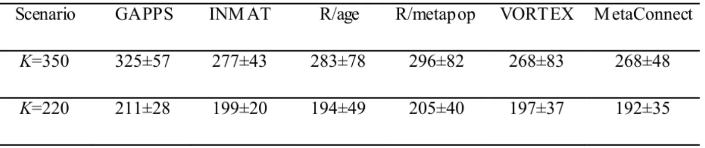
Table II: Estimates of final population size (after 10 years) predicted by software GAPPS, INM AT, RAM AS/age, RAM AS/metapop, VORTEX (Brook et al. 1997) and MetaConnect PVA core modeling. Mean ± standard deviation (as reported by Brook et al. 1997) are given for K=350 and K=220.
Scenario GAPPS INM AT R/age R/metapop VORTEX MetaConnect
K=350 325±57 277±43 283±78 296±82 268±83 268±48
K=220 211±28 199±20 194±49 205±40 197±37 192±35
Validation of the mating system toolbox
Population dynamics model outputs are highly sensitive to the mating system (Doebeli and Koella 1994; Lindstrom and Kokko 1998; Legendre et al. 1999; Calsbeek et al. 2002). Legendre et al. (1999) related the colonization success of invasive passerine birds in New Zealand to their mating system (monogynous vs polygynous). To validate, the mating system toolbox of MetaConnect core modeling, we compared outputs of MetaConnect population dynamics to those obtained by Legendre et al. (1999).
MetaConnect provides results consistent with those provided by Legendre et al. (1999) (Figure 6). The main difference between the models comes from the assumption of the recruitment function. Indeed, Legendre et al. (1999) assume an infinite Malthusian growth function, which is not currently implemented in MetaConnect. Rather, we used a contest recruitment function with K set at 1000 (results not showed), and decreased it to 500 and 250 (Figure 6) to examine the role of setting a constraint on the Malthusian growth rate. Unsurprisingly, for K=1000 results from MetaConnect converged with those obtained by Legendre et al. (1999) under an infinite Malthusian growth function. As the carrying capacity was reduced, extinction probability increased and tended more closely to the pattern observed in the wild. Legendre et al. (1999) suggested that the difference observed between their modeling outputs and the natural observations were probably explained by environmental stochasticity. However, our results suggest that, even though environmental stochasticity may explain a significant part of the discrepancy, the carrying capacity of the population must play
33
a major role in the observed pattern of invasive species extinctions (Figure 6). This agrees with a study of spider extinctions on island where carrying capacity was also found to play a significant role on extinction even in presence of environmental stochasticity (Schoener et al. 2003).
Initial population size
0 100 200 300 400 500 Ex tinctio n pro bability 0.0 0.2 0.4 0.6 0.8 1.0
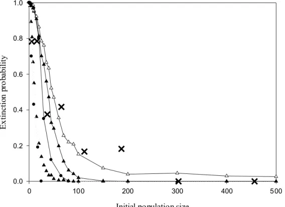
Figure 6: Predicted extinction probability of passerine bird species as a function of the mating system and initial population size. Filled circles correspond to the predictions made by the model used by Legendre et al. (1999) and crosses correspond to natural observations of passerine invasion success in New-Zealand. Triangles are extinction probability estimates provided by MetaConnect. Plain lines correspond to a monogamous mating system and dotted lines to polygynous mating system. Filled triangles are estimates assuming high carrying capacities (K=500) and empty triangles correspond to low carrying capacities (K=250).
Validation of the genetic module
MetaConnect assumes panmixia in local populations (i.e. in patches). Regardless of initial conditions and model assumptions, MetaConnect provides estimates of Fis close to 0. Moreover, simulations considering two patches without dispersal generate a strong genetic
34
structure at the metapopulation scale (Fst≈1) but no structure within local populations (Fis≈0). These two results confirm that the genetic core base of the platform behaves properly.
In addition, we validated the genetic part by comparing the MetaConnect genetic outputs to predictions of the CDPOP model (Landguth and Cushman 2010) in comparable situations. Landguth and Cushman (2010) explored with CDPOP the genetic outcome of three scenarios of landscape structures. The first corresponds to a panmictic population, the second assumes that two patches are isolated by an impassable barrier and the third assumes a simple diffusion model weighted by landscape preference coefficient. Figure 7 shows that results from MetaConnect converged with those obtained by Landguth and Cushman (2010).
Time 0 100 200 300 400 500 Heterozygoz ity m ea sures 0.0 0.2 0.4 0.6 0.8 1.0 CDPOP He CDPOP Ho MetaConnect He MetaConnect Ho CDPOP Ht MetaConnec t Ht Time 0 100 200 300 400 500 Heterozygoz ity m ea sures 0.0 0.2 0.4 0.6 0.8 1.0 Time 0 100 200 300 400 500 Heterozygoz ity m ea sures 0.0 0.2 0.4 0.6 0.8 1.0 B C A
Figure 7: Heterozygosity measures derived from Landguth and Cushman (2010) (long dash) or estimated with MetaConnect (solid lines) under similar dispersal scenarios described in Landguth and Cushman (2010) (A. Panmictic scenario, B. patches are separated by an impassable barrier, C. Individuals navigate between patches in a displacement matrix where rugosity coefficients are comprised between 1 and 63, and dispersers are dispersing following the random walk dispersal rule). For CDPOP and MetaConnect runs, and , the expected and observed heterozygosity can be compared with curves of decay of heterozygosity produced according to Equation 1. The differentiation patterns are similar and variations between MetaConnect results and CDPOP can be attributed to variability between runs and differences in the displacement matrix map used in scenario B and C:
35
Where:
= 4 +
is the observed heterozygosity and , and are respectively the number of males, females and the effective population size.
Model sensitivity:
MetaConnect is a highly flexible IBM which means that dozens of variables can be setup in various modeling context rendering a complete sensitivity analyses impossible to run as with most IBMs (Cross and Beissinger 2001; Naujokaitis-Lewis et al. 2009; Pe'er et al. 2013). Only the mating systems and the dispersal parts of MetaConnect were submitted to sensitivity analysis (see below).
Mating system
Extinction probabilities and allele extinction probabilities are sensitive to the mating system assumption (see Legendre & Clobert 1999 in the validation part above and Moulherat et al. submitted). I will not develop this part here since a complete article is devoted to the implication of the mating system in the model output in a single population that could be reasonably extended to meta-population systems (M oulherat et al. submitted-b).
Landscape resolution, dispersal rule and life strategy impact the outcome linked to dispersal
We studied how landscape structure and resolution will affect dispersal responses in two virtual species with contrasted ecological profiles. The effect of landscape structure was assessed with the virtual landscape designed by Adriaensen et al. (2003), which is a standard arena for testing tools in movement simulations (Chardon et al. 2003; Palmer et al. 2011). In this landscape, we created five suitable habitat patches (ten cells of the grid radius per patch for external patches and a single cell patch for the central one), one at the center and one at the middle of each side of the grid (Figure 8).
36
Figure 8: A. The initial virtual landscape designed by Adriaensen et al. (2003), 1000 X 1000 cells, cell size 1 unit, with four target patches (T1-T4) at equal Euclidean distance from S, the source patch. In the matrix (grid cell resistance R=20), the different structures are to the east a barrier (R=200), to the north a stepping stone like structure of small habitat patch (R=5), to the west a corridor (R=5), and to the south a high resistance zone (R=40). Concerning the habitat patches (S, T1-T4), R=1. B. The simplified virtual landscape used by Palmer et al. (2011) and in this study, 300 X 300 cells, cell size 1 unit. S becomes a one cell patch at equivalent Euclidean distance of T1-T4. The respective resistances of the matrix, the barrier, the stepping stone, the corridor and the high resistance zone are R=10, 100, 1, 1 and 20.
The central patch S was the only one with a permanent population with a carrying capacity of 500 individuals. The four other patches (T1-T4) can host immigrants but their carrying capacity is negative. We have thus a source sink system; the basic idea is to detect how landscape structures in between the central population and the four peripheral ones will affect the immigration rate in the four peripheral ones. Landscape structure are either corridors or stepping stones that are supposed to facilitate dispersal from the central population, or zones with a higher resistance to movements or barriers supposed to impede dispersal from the central population (Figure 8). To describe the sensitivity of MetaConnect to
37
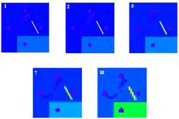
landscape resolution, we reduce the resolution of the modified map of Palmer et al. (2011) by aggregating pixels (Figure 9).
Figure 9: Virtual landscapes of decreasing resolution derived from the initial landscape used by Palmer et al. (2011). The resolution reduction was performed by aggregating respectively 2, 5, 7 and 10 pixels (2-10) of the original map (1). The resistance value of the landscape are represented as a gradient from high (yellow, initially R1,2=100 that reduces in 5, 7 and 10, respectively R5=85, R7=75 and R10=55) to low values (purple, R=0).
The two species released in the landscape differed only in their fecundity. Inter-specific analyses indeed showed that dispersal is traded-off against dispersal ability; species with a high reproductive output (fast species) dispersing less than species with a low reproductive output (slow species) (e.g. Clobert et al. 1998; Stevens et al. 2012). Given the existence of a dispersal polymorphism within species (Stevens et al. 2010), we created two different dispersal strategies for each species: in the short distance dispersal strategy, individuals are able to cross 10% of the grid cells before dying, whereas this threshold increases to 20% for the long distance dispersal strategy. The virtual species has a lizard-like life style with two stages, adults and sub-adults. The survival of both stages was fixed at 0.5, and the fecundity of the slow and the fast species was fixed at 5 and 10 respectively, which provides a stable age structure with 14% and 8% of adults, respectively. Dispersal occurred at