Science Arts & Métiers (SAM)
is an open access repository that collects the work of Arts et Métiers Institute of Technology researchers and makes it freely available over the web where possible.
This is an author-deposited version published in: https://sam.ensam.eu
Handle ID: .http://hdl.handle.net/10985/11888
To cite this version :
Cvetelina VELKOVA, Ivan DOBREV, Michael TODOROV, Fawaz MASSOUH - Approach for numerical modeling of airfoil dynamic stall In: BulTrans2012, Bulgarie, 20120926 -Proceedings of BulTrans-2012, 26-28 September 2012, Sozopol - 2012
BulTrans-2012 Proceedings 26-28 September 2012
Sozopol
APPROACH FOR NUMERICAL MODELING OF AIRFOIL DYNAMIC STALL
CVETELINA VELKOVA
Department of Aeronautics, Technical University, Sofia, Bulgaria [email protected]
MICHAEL TODOROV
Department of Aeronautics, Technical University, Sofia, Bulgaria [email protected]
IVAN DOBREV
Laboratory of Mechanics of Fluids, Arts et Metiers ParisTech, Paris, France
FAWAZ MASSOUH
Laboratory of Mechanics of Fluids, Arts et Metiers ParisTech, Paris, France
[email protected] Abstract:
Aim to the computational study is to present different approach for numerical modeling of airfoil dynamic stall as the airfoil is pitched at a constant rate from zero incidences to a high angle of attack. An application of the Detached-Eddy Simulation model on a NACA 0012 airfoil is presented. The DES model is a method for predicting turbulence in CFD computations, which combines a Reynolds Averaged Navier-Stokes (RANS) method in the boundary layer with a Large Eddy Simulation (LES) in the free shear flow. (DES) turbulence model gives a good accuracy of the flow field because its solves an additional equation for turbulent Reynolds number in a shear stress transport version (SST), which solves a first equation for the turbulent energy K and a second equation for the specific turbulent dissipation rate w. The approach using DES turbulence model is effective because it gives better visualization of flow field, the unsteady separation flow and vortex shedding. Consequently the suggested approach is suitable and it can be used in prediction of dynamic stall phenomenon in the stage of helicopter rotors, wind turbine rotors and aircraft wings design purposes.
Keywords: dynamic stall, unsteady aerodynamics, helicopter rotor, numerical approach
I. Introduction
Dynamic stall is a fluid dynamic phenomenon which occurs during a pitching or plunging of lifting bodies when the static stall angles is exceed. Dynamic stall often appears on helicopter rotor blades, on wings of rapidly maneuvering aircraft, on wind turbine blades or on jet engine compressor blades.
As is summarized in reviews by McCroskey [1] and Carr [2], dynamic stall is characterized with unsteadiness always accompanies the flow over an airfoil at high angle of attack, which is followed by large excursions in lift and pitching moment.
The phenomenon of dynamic stall is very important to the performance and operation of helicopters. Nevertheless much progress has been made nowadays both in analysis and prediction of dynamic stall effects; this physical phenomenon remains a major unsolved problem with a variety of current applications in aeronautics. In order to give some perspective to the present review of dynamic stall, some history of the phenomenon research is in order.
The mechanism of dynamic stall was first identified on helicopters. As is summarized by Carr [2] to underline the importance of unsteady aerodynamics the
first who investigated this event were Harris and Pruyn, [3]. They generalized as a result of further analysis that the extra lift is observed on the helicopter rotor could be explained if lift on the blade was greater than predicted by steady flow during the time when the blade was moving opposite to the direction of flight. As is summarized again by Carr [2], the extra lift could by created by rapid pitching airfoils and that this extra lift was associated with a vortex formed on the airfoil during the unsteady motion. McCroskey [1] verified that the dynamic stall effects were indeed a result of a vortex-dominated flow field that occurred during blade motion into the low-dynamic pressure environment.
As is summarized into the numerical study of dynamic stall by Guilmineau and Queutey, [4] the reason flow field associated with dynamic stall is its dependence on a much large number of parameters: the airfoil shape, Mach number, reduced frequency, amplitude of oscillations, type of motion (ramp and oscillatory), Reynolds number and etc. Because dynamic stall is characterized by large recirculation separated flow regimes, a proper numerical simulation can only be achieved by using the full Navier-Stokes equations with a suitable turbulent viscosity model. CFD methods are shown good capabilities in prediction of 2-D and 3-D dynamic stall events. The primary objective of the
present study is show the different approach for numerical modeling of airfoil dynamic stall using the capabilities and applicability of computational fluid dynamics (CFD) methods.
In the recent years considerable progress have been made in the field of numerical predictions of wind turbine airfoil and blade aerodynamics. Due to the relatively high Reynolds numbers (x(106)) causing RANS methods being the mostapplied if a description of the whole flow field is desired. Even as pressure gradients cause small separated regions, unsteady RANS simulations can predict the flow properly. But during the massive separation, where the flow becomes highly unsteady, both steady and unsteady RANS models fail to predict the correct separation leading to an overestimation of lift. The reason for that is because the RANS simulation produces too much viscosity, which causes a delay of separation leading to a region of attached flow that is too large. Here Large-Eddy Simulation (LES) is in general successful, because LES is filtering of the Navier-Stokes equations, where the large eddies are resolved and only the smaller eddies are modeled. But close to the wall the turbulent eddies is so small and LES is an impractical solution method with respect to computational cost. One way to resolve this is to combine RANS model in the boundary layer with a LES model in farfield. Like is said in [5] the presented method here which is suggested by Spalart et al. [5] is DES. In this study k-ω SST DES is used because it combines the capabilities of RANS and LES modules, and it gives good visualization of the flow-field.
II. Method of Solution
A complexity of dynamic stall and its events such as separation onset, leading-edge vortex shedding and flow reattachment foresees the need of good numerical model that can be used to predict these phenomenon.
For this study to be able to model the airfoil dynamic stall and to see and predict the variation of the unsteady air loads with variations in the oscillatory forcing parameters it is used the experimental data from McCroskey and McAlister [6]. With the variation in parameters such as the amplitude of the angle of attack oscillation, the mean angle of attack α and the reduced frequency can help to provide a better understanding of the physics of described dynamic stall and its events. The used experimental data taken from [6], are the results for NACA 0012 airfoil, take into account [10]. These experimental data summarize the effect on the lift and drag coefficients for increasing α, increasing reduced frequency and increasing Mach number, respectively.
Numerical model representation
The prediction of dynamic stall phenomenon at high
Reynolds number is a crucial need in aeronautics and more specifically in rotorcraft dynamics. Because of the flow and its effects as the forced unsteadiness, random turbulence and produces a strong irreversibility effect that usually leads to hysteresis loops in the aerodynamic coefficients versus the angle of incidence curve, which occur in helicopter rotor blades. Consequently it is important to have a good prediction of the dynamic stall to ensure the efficiency for the design.
It is used a CFD 2d airfoil model with appropriated user-defined function UDF code. UDF is a function that is programmed in C and can be dynamically loaded with FLUENT solver. UDF function has access to all grid and flow variables [7], which are need to calculate the aerodynamic characteristics. Therefore the lift, drag and the pitching moment coefficients for the NACA 0012 are calculated. The validity of suggested numerical approach is checked by comparison between the obtained numerical results with experimental ones, see [6].
For this study, the airfoil performs a sinusoidal pitching motion around the quarter chord point. The mean pitching angle is α0=15°and amplitude of pitch is A=10°. As it is summarized by Leishman in [12], an important parameter that is used to describe the unsteady aerodynamics and unsteady airfoil behavior is the reduced frequency k. This parameter is used to characterize the degree of unsteadiness of the flow. The parameter k is defined in terms of the airfoil semi-chord, b= c/2, where c is the chord of the airfoil, so that
. . 2 w b w c k V V (1)
and ω is angular velocity, V is the local velocity. When k=0, the flow is steady. For 0 ≤ k ≤ 0.05, the flow is quasi-steady; it means that the unsteady effects are usually small. Typically flows with characteristic k≥0.05 are considered unsteady.
As it is summarized by Leishman in [12], for a helicopter rotor in forward flight the reduced frequency is varying on the length of the blade because the local sectional velocity (which appears in the denominator of (1)) is constantly changing. However, as it is concluded by Leishman, [12] a first-order approximation of k can give useful information about the degree of unsteadiness found on the rotor, also the necessity of the modeling unsteady aerodynamic effects in any form of analysis. The reduced frequency in the present study is k = 0.10. The angle of attack is varying by the equation:
0 A.sin t
(2) In this study the unsteadiness of the flow is simulated by the CFD 2d airfoil model, using the function dynamic mesh of FLUENT solver.The initial data are the same as experimental once, [6]. The numerical model represent CFD 2d airfoil model with domain and with suitable grid mesh.
- Airfoil data of NACA 0012
used for modeling taken from [8]. - Grid generation
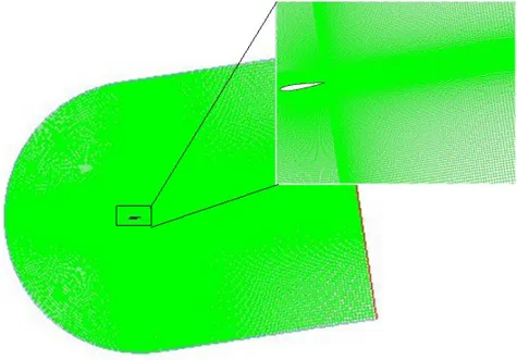
Grid structure and details are shown in Fig. 1 for the mesh used in all calculations in the presented paper, and Fig. 2 to show how it is used the function adapt mesh, for better evaluation of numerical stall angle. The mesh grid on Fig. 1 used is quad map structure mesh, it has 177200 cells and 178 441 nodes. There are 202 nodes on the upper section of airfoil called extrados and the same number to the bottom section – intrados. The quality of the mesh plays a significant role in the accuracy and stability of the numerical computations. Regardless of the type of mesh over the computational domain, checking the quality of mesh is essential. The important indicator of mesh quality that FLUENT allows to check is Wall Ystar, which is 2.7e+01 for the contours of the airfoil in the present study, which is sufficient to give the model capability to ensure better visualization of flow-field in the solution process. The mesh grid was provided for NACA 0012 airfoil. The solving method is iterative. At the begging of the current iteration the CFD 2d airfoil model executes UDF code. The fluid CFD 2d airfoil model clarifies the unsteady flow field around the airfoil, calculating the aerodynamic characteristics of airfoil wake using function dynamic mesh of FLUENT solver. The dynamic mesh function is used for moving the airfoil mesh and the mesh is deformed to each time step.
The time-step size used for the calculation is 15 105
t x
, i.e. over 2500 number of time-steps (2.5 sec) and about 360 positions of pitching airfoil per unit of amplitude or per one period of oscillation T.
Fig. 2 Mesh – adapt over the nose of the airfoil The SIMPLE algorithm is employed for the pressure/velocity coupling and solution of the momentum equations is obtained using a Bounded Central Differencing scheme. Unsteady computations are made with a second order dual time stepping algorithm, which is stable for large time steps and thereby decreases the computational time. Various turbulence models are available in CFD code, but here DES k-ω SST model has proven quite suitable for airfoil flows. See [9]
III. Results and analysis
The obtained numerical results are presented in Fig. 3, Fig. 4, Fig. 5 and Fig. 6.
DES k- ω SST turbulence model used for Fig. 1 The mesh over the airfoil domain and grid near the airfoil
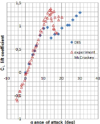
calculations is hybrid model. The k-ω SST turbulence model is used to model the flow near to the airfoil. DES is using, because it visualize the flow field well at high angle of attack α, see Fig. 3, Fig. 4. The experimental static lift data in Fig. 3, taken from [6] show the static characteristic of the NACA 0012 airfoil. It’s worth to mention that the obtained numerical results are for unsteady flow. Fig. 3 represents the made comparison between experimental static lift coefficient and obtained numerical results. This case in Fig. 3 from the present study used DES k- ω SST turbulence model with the same grid as it is used for calculation of lift coefficient CL in Fig. 4, but without moving mesh. For the evaluation of CL presented in Fig. 4, it is used function dynamic mesh.
The obtained numerical results for aerodynamic characteristics of lift coefficient CL and drag coefficient CD are approximated well with the experiment data; see Fig. 4 and Fig. 5. But the suggested DES k- ω SST turbulence model is not given the good estimation of stall angle. It can be observed from Fig. 3, where obtained numerical results from the calculations shown that the stall angle is lower than the actual stall angle on the experimental curve of CL, see Fig. 3.
When it is observed the slope of CL and CD, in Fig. 4 and Fig. 5, it can be noted that after the stall angle, the flow becomes unsteady and the values of CL and CD, are varying with the time. The fluctuations, which are observed on the curve of lift and drag coefficient, see Fig. 4 and Fig. 5 in angles of attack higher than α=20° confirm the unsteadiness of the flow field after stall angle. Because of that it is made a comparison between averaged computational values of lift coefficient for experimental data, obtained numerical results and the results obtained by Martinat, [9] and the hysteresis loops on CL, see Fig. 4 and CD, see Fig. 5.
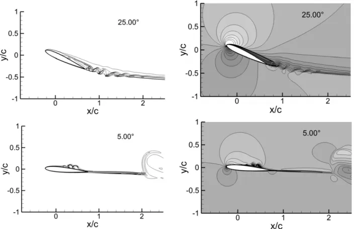
Fig. 6 illustrated iso-vorticity fields (left) and velocity magnitude (right) at 25° angle of incidence upstroke and 5° angle of incidence downstroke for two-dimensional DES k-ω SST modeling. As it is observed in Fig. 6 the flow is fully stalled at 25° angle of incidence. Therefore it can be conclude that the numerical simulations predict that the stall angle is 25° which is 1° or 2° more than the stall angle of attack for the experiment curve of CL and CD given in Fig. 4 and Fig. 5. But the contraction of the velocity’s streamlines on the back of upper surface on the airfoil to the end in Fig. 6 (right) at 25° indicates the increasing of leading edge vortex. But starting airfoil oscillations in downstroke, it is supposed that the flow over the airfoil progress to a state of full separation during the downstroke.
Fig. 3 Comparison between static lift data on the NACA 0012 for experiment and DES
Fig. 4 Comparison between lift hysteresis on the NACA 0012 for experiment, k-ω SST model and DES
Fig. 5 Drag coefficient versus mean pitching angle, DES
IV. Conclusion and Recommendation
In the considered cases of the present study, although DES k- ω SST turbulence model is usually used for three-dimensional computations flow, here this model is shown to capture the two-dimensionality of flow physics well. Because of the relatively good correspondence between experimental data and obtained airfoil characteristics, it supposes the proper choice of methodologies including differencing scheme and grid resolution. Therefore, it can be concluded that the use of DES k-ω SST hybrid model capture comparatively well the dynamic stall region for 2-D computations of pitching airfoil NACA 0012.
In the future it is recommended, the investigation to be focus on the three-dimensional computations. The last recommendation is in order to see if the present approach is applicable for the problems of helicopter rotor dynamics and more specifically for the dynamic stall. It can be investigate the capability of model to capture the dynamic stall regions using LES turbulence model.
Fig. 6 Iso-vorticity fields (left) and velocity magnitude with streamlines (right) at 25° of incidence upstroke and 5° of incidence downstroke for two-dimensional DES k-ω SST modeling
Acknowledgements
This study has been supported by Research and Development Direction of Technical University of Sofia (Grant 122PD0001-04/2012).
References:
[1] McCroskey, W. J., “The Phenomenon of Dynamic Stall,” NACA TM-81264, March 1981.
[2] Carr, L. W., “Progress in Analysis and Prediction of Dynamic Stall, ” Journal of Aircrafts, Vol. 25, No. 1, 1988, pp. 6-17.
[3] Harris, F.D. and Pruyn, R.R., “Blade Stall-Half Fact, Half Fiction,” Journal of the American Helicopter Society, Vol. 13, No. 2, April 1968, pp. 27-48.
[4] Guilmineau, E., Queutey, P., “Numerical Study of Dynamic Stall on Several Airfoil Sections,” AIAA Journal, Vol. 37, No. 1, 1994
[5] Johansen, J., Sorensen, N.N, “Application of a Detached-Eddy Simulation model on Airfoil Flows,” IEA 2000
[6] McCroskey W. J., McAlister K. W., Carr L. W. and Pucci S. L., “An Experimental Study of Dynamic Stall on Advanced Airfoil Sections Volume 1.Summary of the Experiment,” p.98, Fig. 35, NASA, July 1982.
[7] Dobrev I., Massouh F., “Actuator surface hybrid model,” ENSAM Laboratoire de Mecanique des Fluides, Journal Physics, 2007.
[8]
http://www.ae.illinois.edu/m-elig/ads/coord_database.html
[9] Martinat G., Hoarau Y., Braza M., Vos J. and Harran G., “Numerical Simulation of the Dynamic Stall of a NACA 0012 Airfoil Using DES and Advanced OES/URANS Modeling,” 2008.
[10] McAlister K. W., Carr L. W and McCroskey W. J., “Dynamic Stall Experiments on the NACA 0012 Airfoil”, NASA Technical Paper 1000, January 1978.
[11] Fluent Inc., “FLUENT 6.3 User’s Guide”,© Fluent Inc, 2006.
[12] Leishman J. G., “Principles of Helicopter Aerodynamics”, Cambridge Aerospace Series