L'ionosphère du côté nuit de Mars dévoilée par les déplétions d'électrons suprathermiques

THÈSE

En vue de l’obtention du

DOCTORAT DE L’UNIVERSITÉ DE TOULOUSE

Délivré par :

Université Toulouse III - Paul Sabatier (UT3 Paul Sabatier)

Présentée et soutenue par :

Morgane STECKIEWICZ

Le Mardi 26 Septembre 2017

Titre :

L’ionosphère du côté nuit de Mars dévoilée par les déplétions

d’électrons suprathermiques

École doctorale et discipline ou spécialité :

ED SDU2E : Astrophysique, Sciences de l’Espace, Planétologie

Unité de recherche : IRAP Directeur/trice(s) de Thèse : Jury : Christian MAZELLE Nicolas ANDRÉ Philippe GARNIER Directeur de Recherches Chargé de Recherches Maître de conférences Directeur de thèse Co-directeur de thèse Encadrant de thèse François LEBLANC Dominique DELCOURT Viviane PIERRARD Sébastien BOURDARIE Dominique FONTAINE Directeur de Recherches Directeur de Recherches Maître de Recherches Maître de recherches Directrice de Recherches Président du jury .Rapporteur Rapporteur Examinateur N.CExaminateur

The nightside Martian ionosphere

unveiled by suprathermal electron

‘La plus utile et honorable science et occupation A une femme, c’est la science du ménage.’

Acknowledgements

I would like first to thank MAVEN, which achieved with success its insertion around Mars and records for more than three years now wonderful data without which this PhD would not have occurred. We began our research life together and I hope its will last much longer. Through this acknowledgement I obviously want to thank the operation and instrument teams, as well as the science team which welcomed me among them. Among others I would like to thank Bruce Jakosky, Dave Brain, Jasper Halekas, Jared Espley, Jim McFadden, and Jack Connerney for the help they gave me all along this PhD. A special acknowledgement to Janet Luhmann, Dave Mitchell, Rob Lillis and Laïla Andersson who followed my work from the beginning, helped me write my papers and are always good advisors in the way to carry on studies. I would also like to thank Shannon Curry, Gina DiBraccio, Yasir Soobiah, Yuki Harada, Shaosui Xu, Yaxue Dong, Yuni Lee, Scott England, Zachary Girazian, Christopher Fowler, Matt Fillingim and Meridith Elrod for the interesting discussions and the moments spend together.

Je remercie profondément Dominique Fontaine et Sébastien Bourdarie d’avoir accepté de participer à mon jury, François Leblanc de l’avoir présidé, ainsi que les rapporteurs Viviane Pierrard et Dominique Delcourt pour leurs lectures attentives, leurs remarques et leurs conseils. Merci infiniment à tous. I also want to thank Dave Mitchell for his coming, his kindness and his picky questions. Je remercie également Dorine Roma pour avoir organiser les déplacements des différents membres du jury.

Je remercie mes directeurs de thèse pour m’avoir donné l’opportunité de faire ce doctorat et tout particulièrement Philippe, qui a accepté de faire partie de cette aventure périlleuse et qui m’a suivie, épaulée, encouragée et soutenue tout au long de ces trois années. Merci pour ton temps et tes conseils, et surtout pour avoir donné une chance à cette thèse. Je tiens aussi à remercier Ronan et François pour leur gentillesse et leur bienveillance, mais aussi pour le temps qu’ils ont consacré à mes travaux.

Cette thèse a été effectuée au sein de l’IRAP et je tiens à remercier ses directeurs successifs Martin Giard et Philippe Louarn pour m’avoir accueilli dans leur laboratoire. J’ai ainsi pu profiter de toute l’infrastructure du laboratoire pour mener à bien ce travail. Je suis profondément reconnaissante à tous les membres de l’équipe PEPS pour m’avoir acceptée

parmi eux et encouragée tout au long de ces trois années. Merci notamment à Benoit, Aurélie, Jérémie, Christian J., Matthieu, Andréi, Frédéric, Alexis, Pierre-Louis, Iannis, Lionel, Vincent et Jeannot. Je remercie en particulier Jean-André Sauvaud pour avoir été ma voix quand celle-ci n’était pas à la bonne fréquence, et pour m’avoir permis de publier mon premier article. Mercelle-ci à Dominique Toublanc pour son soutien et ses conseils tout au long de ma thèse et de mon parcours dans l’enseignement. Merci à Arnaud pour m’avoir soutenue dans les premiers mois de ma thèse et mes premières missions. Merci à Myriam et Elena pour avoir sauvé je ne sais combien de Time Tables et plus globalement merci aux équipes de développement informatique pour m’avoir facilité l’accès aux données tout au long de ma thèse.

Dans un ordre non représentatif : Merci à UniverSCiel et à tous ses membres pour leur dynamisme, leur enthousiasme, leur gentillesse et tous les projets passionnants qu’ils portent et auxquels j’ai pu participer pour faire briller un peu plus les yeaux des enfants (et des grands enfants). Merci en particulier à Marina, Wilhem, Vincent, Philippe, Edoardo, Damien, Tata, Minus et Cortex pour ces moments passés ensemble. Merci aux Etoiles brillents pour tous et à Thierry, Pieter, Cécile, Armelle, Emmy, Simon, Julie, Mélanie et Hélène pour cette expérience unique ! Merci à Geneviève pour m’avoir suivie et aidée dans les divers choix difficiles que j’ai été amené à prendre depuis quatre ans. Merci à Marie Brut et à Jean-François Georgis de m’avoir fait découvrir l’enseignement. Merci à Natasha, Benjamin, Thomas et Mika d’avoir partagé mon bureau tout au long de ces trois années. Merci pour ces moments et rires partagés. Merci à Myriam, Gaëlle, Elsa et David pour toutes les pauses café que nous avons partagées. Merci à Merlin pour sa participation à l’écriture de ma thèse. Merci à Agnès pour m’avoir aidé à préparer ma soutenance et pour son soutien. Je suis très heureuse d’avoir pu faire ces conférences sur Mars avec toi  Merci à Issaad pour m’avoir nourrie de gateaux délicieux ! Merci à Mikel, Mickaël, Nathanaël, Maxime, Anna, Norberto, Yoann, Eduardo et Jérémy pour votre écoute votre gentilesse, et les moments passés ensembles. Merci également à Zonta International pour avoir reconnu la valeur de mes travaux à travers la bourse Amelia Earhart. Je suis très heureuse que cette thèse m’ait permi de tous vous rencontrer.

Enfin, merci à ma famille, mes parents, mes grands-parents, mes sœurs, mon neuveu et mes nièces, mais surtout merci à Arthur pour avoir été là tous les jours de ma thèse, pour m’avoir soutenu et permis d’arriver jusqu’au bout de cette épreuve.

Abstract

The nightside ionosphere of Mars still remains an unfamiliar and mysterious place. Nightside suprathermal electron depletions are specific features of this region which have been observed at Mars by three spacecraft to date: Mars Global Surveyor (MGS), Mars EXpress (MEX) and the Mars Atmosphere and Volatile EvolutioN (MAVEN) mission. Their study enables the observation of the nightside ionosphere structure and dynamics as well as the underlying neutral atmosphere, the specific Martian magnetic topology, and possible conduits for atmospheric escape. Structures as different as magnetic cusps, current sheets or the UV terminator can be investigated through suprathermal electron depletions, due to the processes leading to their observation on the nightside of Mars.

The main goal of my PhD has been to use the complementarity of the three missions MGS, MEX, and MAVEN to understand the different mechanisms at the origin of suprathermal electron depletions and their implication on the structure and the dynamics of the nightside ionosphere. In this context, three simple criteria adapted to each mission have been implemented to identify suprathermal electron depletions from 1999 to 2017.

A statistical study reveals a transition region near 170 km altitude separating the collisional region where suprathermal electron depletions are directly due to electron absorption by atmospheric CO₂ and the collisionless region where they are mainly due to electron exclusion by closed crustal magnetic field loops. Understanding of these phenomena enables me to estimate the location of the UV terminator. It appears to be located ~120 km above the optical terminator, though this location is different between the dawn and dusk terminator and is expected to vary throughout the different Martian seasons.

Résumé

L’ionosphère du côté nuit de Mars reste encore à ce jour une zone mystérieuse et peu connue de l’environnement Martien. Les déplétions d’électrons suprathermiques sont des structures spécifiques à cette région, observées jusqu’à présent par trois satellites : Mars Global Surveyor (MGS), Mars EXpress (MEX) et Mars Atmosphere and Volatile EvolutioN (MAVEN). Leur étude permet aussi bien l’observation de la structure et de la dynamique de l’ionosphère du côté nuit que celle de l’atmosphère neutre, de la topologie magnétique martienne, ainsi que l’étude de l’échappement atmosphérique de Mars. Des structures aussi différentes que les cornets magnétiques, les couches de courants ou encore le terminateur ultra-violet peuvent être examinées à travers les déplétions d’électrons suprathermiques, de par les mécanismes à l’origine de leur présence du côté nuit de Mars.

Le but principal de ma thèse a été de tirer parties des trois jeux de données offerts par les satellites MGS, MEX et MAVEN pour mieux comprendre les mécanismes à l’origine des déplétions d’électrons suprathermiques observées du côté nuit ainsi que leur impact sur la structure et la dynamique de l’ionosphère du côté nuit. Dans cette optique, trois critères simples adaptés à chaque mission ont été développés pour identifier les déplétions d’électrons suprathermiques dans une base de données allant de 1999 à 2017.

Une étude statistique a révélé la présence d’une région de transition autour de 170 km d’altitude séparant la région collisionnelle dans laquelle les déplétions d’électrons suprathermiques sont directement dues à l’absorption des électrons par le CO2 atmosphérique,

et la région non-collisionnelle dans laquelle elles sont principalement dues aux boucles fermées de champs magnétique d’origine crustale. La compréhension de ces mécanismes m’a permis d’estimer la localisation du terminateur ultra-violet. Celui-ci est situé en moyenne ~120 km au-dessus du terminateur optique. Cette altitude varie entre le côté soir et le côté matin, et une variation saisonnière est prédite par les modèles atmosphériques.

Table of Contents

Acknowledgements ______________________________________________ 5

Abstract _______________________________________________________ 7

Résumé ________________________________________________________ 8

Introduction ___________________________________________________ 14

Introduction ___________________________________________________ 17

1.

The Martian environment ____________________________________ 20

1.1. Interaction of the solar wind with the different bodies of the Solar System ___ 20

1.1.1. The solar wind __________________________________________________ 20 1.1.2. Four different classes of interaction _________________________________ 22

1.2. The Martian obstacle _______________________________________________ 29

1.2.1. Mars today _____________________________________________________ 29 1.2.1.1. Atmosphere - Exosphere - Ionosphere: who is who? ________________ 29 1.2.1.2. The Martian magnetic field ____________________________________ 34 1.2.2. Back to the history of Mars ________________________________________ 38 1.2.2.1. A magnetic field history _______________________________________ 39 1.2.2.2. A Mars’ volatile and climate history _____________________________ 41

1.3. The interaction of the solar wind with Mars ____________________________ 45

1.3.1. The steady-state interaction ________________________________________ 48 1.3.1.1. The bow shock and the upstream region __________________________ 49 1.3.1.2. The magnetosheath __________________________________________ 51 1.3.1.3. The Magnetic Pile-up Boundary and the Magnetic Pile-up Region _____ 52 1.3.1.4. The ionopause and the PhotoElectron Boundary ____________________ 54 1.3.1.5. The ionosphere ______________________________________________ 55 1.3.1.6. The wake and the magnetotail __________________________________ 56 1.3.2. Dynamics of the Martian interaction with the Sun ______________________ 58 1.3.2.1. Martian magnetic topology ____________________________________ 58 1.3.2.2. Pressure balance _____________________________________________ 59 1.3.2.3. Variability of the boundaries ___________________________________ 60 1.3.3. Focus on the nightside ionosphere __________________________________ 62

2.

Instrumentation, data and analysis tools used ____________________ 66

2.1. Exploration of Mars ________________________________________________ 66

2.1.1. Mars Global Surveyor ____________________________________________ 68 2.1.1.1. Scientific objectives __________________________________________ 68 2.1.1.2. Orbitography _______________________________________________ 69 2.1.1.3. Instruments _________________________________________________ 70 2.1.1.4. Main discoveries ____________________________________________ 71 2.1.2. Mars Express ___________________________________________________ 73 2.1.2.1. Scientific objectives __________________________________________ 73 2.1.2.2. Orbitography _______________________________________________ 74 2.1.2.3. Instruments _________________________________________________ 75 2.1.2.4. Main discoveries ____________________________________________ 76 2.1.3. MAVEN ______________________________________________________ 78 2.1.3.1. Scientific objectives __________________________________________ 78 2.1.3.2. Orbitography _______________________________________________ 79 2.1.3.3. Instruments _________________________________________________ 81 2.1.3.4. Main discoveries ____________________________________________ 83 2.2. Instrumentation ____________________________________________________ 85

2.2.1. Mars Global Surveyor ____________________________________________ 85 2.2.1.1. The magnetometer: MAG _____________________________________ 85 2.2.1.2. The Electron Reflectometer: ER ________________________________ 85 2.2.2. Mars Express ___________________________________________________ 88 2.2.2.1. Electron Spectrometer: ELS ___________________________________ 88 2.2.2.2. The ion spectrometer: IMA ____________________________________ 90 2.2.3. MAVEN ______________________________________________________ 91 2.2.3.1. The ion spectrometer: STATIC _________________________________ 92 2.2.3.2. The Magnetometer: MAG _____________________________________ 93 2.2.3.3. The Electron spectrometer: SWEA ______________________________ 94 2.2.3.4. The Langmuir probe: LPW ____________________________________ 97 2.2.4. Contamination __________________________________________________ 99

2.3. Data coverage ____________________________________________________ 102

2.4.1. AMDA and 3D view ____________________________________________ 105 2.4.2. CL __________________________________________________________ 106

2.5. Frames __________________________________________________________ 107

2.5.1. The Mars-centric Solar Orbital (MSO) frame _________________________ 107 2.5.2. The IAUMars frame _____________________________________________ 107

2.5.3. Definition of the altitude _________________________________________ 108 2.5.4. Definition of the nightside ________________________________________ 108

2.6. Model of crustal magnetic field: the model of Morschhauser et al. [2014]____ 110

3.

Identification of suprathermal electron depletions in the nightside

ionosphere _______________________________________________ 113

3.1. A story of depletions _______________________________________________ 113

3.1.1. Discovery of electron depletions ___________________________________ 113 3.1.2. On the origin of plasma voids _____________________________________ 117 3.1.3. Global properties of the plasma voids observed by MGS and MEX _______ 120

3.2. General properties of electron depletions observed with MAVEN _________ 122

3.2.1. Plasma voids or suprathermal electron depletions? ____________________ 122 3.2.2. Plasma composition _____________________________________________ 125 3.2.2.1. Ions characteristics __________________________________________ 125 3.2.2.2. Electrons characteristics ______________________________________ 127 3.2.3. An overview of the variety of the flux spikes _________________________ 128 3.2.4. Are electron depletions really related to crustal fields? _________________ 129

3.3. Automatic detection of suprathermal electron depletions: definition of the criteria __________________________________________________________ 132

3.3.1. MAVEN _____________________________________________________ 132 3.3.2. MEX ________________________________________________________ 134 3.3.3. MGS ________________________________________________________ 135

3.4. Application of the criteria __________________________________________ 136

3.4.1. Application to MGS ____________________________________________ 136 3.4.2. Application to MAVEN _________________________________________ 137 3.4.2.1. Application of criterion (1) ___________________________________ 137 3.4.2.2. MAVEN coverage __________________________________________ 138

3.4.3. Application to MEX ____________________________________________ 140 3.4.3.1. Unrestricted application ______________________________________ 140 3.4.3.2. Restricted application ________________________________________ 143

4.

On the processes at the origin of suprathermal electron depletions _ 145

4.1. Altitude dependence of the distribution of suprathermal electron depletions 145

4.1.1. Altitude distribution of the electron depletions observed by MAVEN ______ 145 4.1.2. Geographical distribution of suprathermal electron depletions: a common vision from above 250 km ____________________________________________ 147 4.1.2.1. Geographical distribution at 400 km ____________________________ 147 4.1.2.2. Geographical distributions from 250 km to 900 km ________________ 151 4.1.3. Going down to 125 km altitudes with MAVEN _______________________ 156 4.1.3.1. From 250 to 170 km _________________________________________ 156 4.1.3.2. Below 170 km _____________________________________________ 158

4.2. A competition between two main loss processes ________________________ 161

4.2.1. Plasma composition of suprathermal electron depletions ________________ 161 4.2.2. The role of crustal magnetic sources ________________________________ 166

4.2.2.1. Comparison between the northern and southern hemispheres with both MAVEN and MEX _________________________________________ 166 4.2.2.2. Evolution of the altitude distribution of electron depletions with crustal

magnetic field amplitude ____________________________________ 168 4.2.2.3. Pressure balance ____________________________________________ 170

4.3. Discussion on the altitude of the electron exobase _______________________ 174

4.3.1. Updated scenario of creation of suprathermal electron depletions _________ 174 4.3.2. Evolution of the altitude of the exobase with the Solar Zenith Angle ______ 176

5.

Around the holes: the dynamics of the nightside ionosphere _______ 178

5.1. Where the electron depletions stop: the flux spikes ______________________ 178

5.1.1. Injection of ionospheric plasma ___________________________________ 179 5.1.2. Energy-time dispersed electron signature ____________________________ 182 5.1.3. Current sheet crossing at low altitudes ______________________________ 187

5.2. Unexpected (non-)observations of suprathermal electron depletions _______ 191

5.2.1.1. An altitude issue ____________________________________________ 191 5.2.1.2. A spacecraft charging issue ___________________________________ 192 5.2.2. Non-observation of electron depletions at low altitudes _________________ 193 5.2.2.1. Different types of orbits with no electron depletion ________________ 194 5.2.2.2. Distribution of the 61 events in the Martian environment ____________ 199 5.2.2.3. Focus on the Tharsis region ___________________________________ 204

5.3. Where suprathermal electron depletions reveal the UV terminator ________ 209

5.3.1. Observation of the UV terminator __________________________________ 209 5.3.1.1. Distribution of electron depletions as a function of SZA ____________ 210 5.3.1.2. Review of the nightside definition ______________________________ 211 5.3.1.3. Observation of the UV terminator with LPW and SWEA ____________ 212 5.3.1.4. Back to suprathermal electron depletions ________________________ 214 5.3.2. Determination of the average altitude of the UV terminator______________ 215 5.3.2.1. Distribution of electron depletions over one Martian year ___________ 216 5.3.2.2. Methodology ______________________________________________ 217 5.3.2.3. Results and comparison with model ____________________________ 218 5.3.3. Evolution of the UV terminator with seasons: the dawn- dusk asymmetry __ 219 5.3.3.1. Predictions from the model of Robert Lillis ______________________ 220 5.3.3.2. Results obtained with electron depletions ________________________ 222 5.3.3.3. Focus on the equinox of 2016 _________________________________ 224 5.3.3.4. The mystery of the reversal at the aphelion and perihelion ___________ 226

Conclusions and Perspectives ____________________________________ 230

Conclusions et Perspectives _____________________________________ 233

Acronyms ____________________________________________________ 237

Table of figures _______________________________________________ 239

Table of tables ________________________________________________ 242

Bibliography _________________________________________________ 243

Appendices ___________________________________________________ 256

Introduction

The nightside ionosphere of Mars is still poorly investigated compared to the dayside one. One of the main observational properties of this region is the presence of recurrent structures characterized by significant depletions in electron fluxes and hence called “nightside suprathermal electron depletions” (hereinafter referred to as electron depletions). The first observations of these structures were obtained during the 400 km mapping orbit of Mars Global Surveyor (MGS) by the Electron Reflectometer instrument that detected on Mars’ optical shadow pronounced decreases of the electron count rates up to three orders of magnitude at all energies [Mitchell et al., 2001]. The same structures were then detected by the Mars Express (MEX) Electron Spectrometer [Soobiah et al., 2006]. The statistical analysis of their geographical distribution suggested that the observation of electron depletions is due to the passage of the spacecraft inside closed crustal magnetic field loops preventing plasma coming from the dayside or the magnetotail from populating these regions. [Mitchell et al., 2001;

Soobiah et al., 2006; Soobiah, 2009]. However, studies on electron depletions made with MGS and MEX are both restricted in altitude and instrumentation. They cannot observe the phenomenon at altitudes below 250 km with a complete suite of plasma instruments.

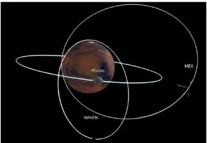
On September 21, 2014, a new spacecraft get inserted around Mars to complement the Martian fleet: the Mars Atmosphere and Volatile EvolutioN (MAVEN) mission. It is designed to study the structure, composition, and variability of the upper atmosphere and ionosphere of Mars, its interaction with the Sun/solar wind, and the Martian atmospheric escape [Jakosky et al., 2015a]. For this purpose, it carries onboard a complete suite of plasma and field instruments including a magnetometer, two ion and one electron spectrometers, and a Langmuir probe. The spacecraft since then reached its mapping orbit which is a highly elliptical precessing orbit with a nominal periapsis at 150 km, a period of 4.5 h and an inclination of 75°. This periapsis can periodically be lowered down to ~125 km for 5 days periods known as “deep-dips”, which allows measurements of suprathermal electron depletions at previously unsampled altitudes.

Contrary to MGS and MEX observations, during most MAVEN periapsis passages in the nightside ionosphere suprathermal electron depletions are detected, even in regions with nearly no crustal magnetic field. Hence, MGS and MEX only observed the tip of the iceberg. Other processes than the interaction with crustal magnetic fields must occur for suprathermal electron depletions to be observed.

Suprathermal electron depletions are interesting structures as they are recurrently observed on the nightside ionosphere and can be used to characterize its structure and dynamics.

Mitchell et al., [2007] and Brain et al., [2007] for example used electron depletions to determine the magnetic topology of Mars thanks to electron spectrometers. However, a clear comprehension of the processes at the origin of the observation of these structures is lacking and needed to carry out such studies.

In this work I want to take advantage of the different datasets offered by MGS, MEX and MAVEN to better understand the structure and dynamics of the nightside ionosphere through the study of electron depletions. MGS data are therefore used from 1999 to 2006 to take advantage of the mapping circular orbit at a roughly constant altitude (~400 km) of the spacecraft, allowing observations of the phenomenon every 2 h over the whole range of possible latitudes [-90°, 90°]. MEX data are used from 2004 to 2014, which gives us an unparalleled

long-term view of the phenomenon at both relatively low (down to ~250 km) and high

altitudes. Finally, MAVEN data are used from October 2014 to March 2017. During this time period the spacecraft covered both hemispheres except the poles, but due to this short duration and MAVEN orbital parameters, all latitudes are not yet covered at all possible altitudes. Even though the coverage and duration of this data set are much lower than those of MGS and MEX, MAVEN reached during this time period altitudes down to 110 km, which are unsampled by MGS nor MEX. Added to MAVEN instrument suite, this coverage enable a finer study of the structure of suprathermal electron depletions. This huge data set gathering observations made over 18 years by different instruments reaching different altitude regimes enables us to compare events observed in similar conditions (several spacecraft in the same region) and enrich this joint vision with new observations closer to the surface (with MAVEN).

So as to present the work carried out during my PhD, this manuscript is divided into five chapters:

 In Chapter 1 is described the global environment of Mars: what characterizes the Martian obstacle, how it interacts with the solar wind, what are the regions and boundaries we are likely to encounter when looking at plasma data, to finally focus on the nightside ionosphere and its suprathermal electron depletions.

 In Chapter 2 are described the different datasets used in this manuscript: we browse the different missions and their associated orbitography and instruments, the analysis tools I have used to process the data, the frames and definitions that I will use in the rest of the manuscript and the model of crustal magnetic field that I have chosen.

 Chapter 3 is dedicated to the identification of suprathermal electron depletions. These structures have already been identified by several spacecraft and instruments but the MAVEN payload offers new highlights on their properties. This enables me to create criteria able to automatically detect suprathermal electron depletions in the different electron spectrometers data.

 In Chapter 4 I use the catalogs obtained after application of the three criteria to characterize the different processes at the origin of suprathermal electron depletions in the nightside ionosphere of Mars. Geographical and altitudinal distributions are used in association with pressure balance and plasma composition analysis in order to derive an updated scenario of creation of electron depletions.

 In Chapter 5 I focused on the dynamics of the nightside ionosphere. The flux spikes regularly observed between suprathermal electron depletions are structures of interest to observe the dynamics of the nightside ionosphere. The observation of electron depletions in unexpected regions or the absence of observation in regions where they should cover the whole surface regarding the previously established scenario remind us that other processes are at work in the nightside ionosphere. The location of the UV terminator, and its variability with seasons and dusk/dawn side are investigated.

Introduction

L’ionosphère du côté nuit de Mars est une partie assez peu connue de l’environnement martien, comparée à l’ionosphère du côté jour. Une des principales caractéristiques observationnelles de cette région est la présence de structures récurrentes caractérisées par une déplétion significative du flux d’électrons. Elles sont pour cette raison appelées « déplétions d’électrons suprathermiques du côté nuit » (nous les appellerons par la suite déplétions

d’électrons pour ne pas alourdir le texte). La première observation de ces structures a été

réalisée par le satellite Mars Global Surveyor (MGS) dont l’orbite était circulaire à ~400 km. Son spectromètre à électrons détecta de fortes diminutions du taux de comptage d’électrons jusqu’à trois ordres de grandeur à toutes les énergies quand le satellite passait dans l’ombre de la planète [Mitchell et al., 2001]. Le même type de structures a ensuite été détecté par le spectromètre à électrons du satellite Mars Express (MEX) [Soobiah et al., 2006]. Une étude statistique de leur distribution géographique suggéra que l’observation de déplétions d’électrons est due au passage du satellite dans des boucles fermées de champ magnétique crustal excluant le plasma venant du côté jour ou de la queue [Mitchell et al., 2001; Soobiah et al., 2006; Soobiah, 2009]. Cependant, les études menées sur les déplétions d’électrons à l’aide des données de MGS et de MEX sont à la fois restreintes en altitude et au niveau instrumental. Ces satellites ne peuvent en effet observer ce phénomène qu’à des altitudes supérieures à 250 km, avec une instrumentation ne permettant qu’une étude partielle de ses caractéristiques.

Le 21 Septembre 2014 un nouveau satellite est entré en orbite autour de Mars, complétant ainsi la flotte martienne : la mission Mars Atmosphere and Volatile EvolutioN (MAVEN). Cette mission a pour but d’étudier la structure, la composition et la variabilité de la haute atmosphère et de l’ionosphère martienne, leurs interactions avec le Soleil et le vent solaire ainsi que l’échappement atmosphérique de Mars [Jakosky et al., 2015a]. Dans cette optique, MAVEN a embarqué à son bord un ensemble cohérent d’instruments plasma, dont deux magnétomètres, deux spectromètres à ions et un à électrons, et une sonde de Langmuir. Le satellite est sur une orbite fortement elliptique, précessant naturellement, avec un périapse nominal à 150 km, une période de 4,5 h et une inclinaison de 75°. Ce périapse peut périodiquement être abaissé pour atteindre une altitude de ~125 km pendant une période de cinq jours appelée « deep dip ». Ces périodes permettent d’effectuer des observations de déplétions d’électrons à des altitudes jamais atteintes précédemment.

Jusqu’à présent, des déplétions d’électrons ont été observées avec MAVEN au cours de tous ses passages à basses altitudes du côté nuit, sauf quelques rares exceptions, et ce même dans les régions où le champ magnétique d’origine crustale est très faible. Ainsi, il semble que MGS et MEX n’aient pu observer que la partie émergée de l’iceberg. L’interaction du plasma avec le champ magnétique crustal ne peut pas être le seul mécanisme à l’origine de la création de déplétions d’électrons.

Les déplétions d’électrons sont des structures intéressantes de par leur observation récurrente dans l’ionosphère du côté nuit de Mars. Elles peuvent ainsi être utilisées pour caractériser sa structure et sa dynamique. Mitchell et al., [2007] et Brain et al., [2007] les ont par exemple utilisées pour déterminer la topologie magnétique de Mars à l’aide des données issues des spectromètres à électrons. Cependant, une bonne compréhension des processus à l’origine de la formation des déplétions d’électrons manque et est nécessaire pour mener à bien de telles études.

A travers ce doctorat j’ai souhaité tirer au maximum profit des différents jeux de données offerts par MGS, MEX et MAVEN pour mieux comprendre la structure et la dynamique de l’ionosphère du côté nuit de Mars à travers l’étude des déplétions d’électrons. Dans cette optique, les données de MGS ont été utilisées de 1999 à 2006, de sorte à tirer profit de son orbite circulaire, permettant une observation du phénomène toutes les deux heures sur toute la gamme de latitude possible [-90° ; 90°]. En ce qui concerne MEX, j’ai utilisé les données obtenues entre 2004 et 2014, ce qui donne une vue à long terme du phénomène, à la fois à relativement basses altitudes (jusqu’à ~250 km) et à hautes altitudes. Finalement, les données de MAVEN ont été utilisées d’Octobre 2014 jusqu’à Mars 2017. Pendant cette courte période le satellite a couvert les deux hémisphères à l’exception des pôles. Cependant, cela n’est pas encore suffisant pour couvrir toutes les latitudes à toutes les altitudes possibles. Bien que la couverture et la période étudiée soit bien plus faible que pour MGS et MEX, MAVEN est descendu pendant cette période jusqu’à des altitudes de 110 km, altitudes non couvertes ni par MGS ni par MEX. Cette couverture, associée aux capacités instrumentales de MAVEN, permet une étude plus fine des déplétions d’électrons suprathermiques. Cette immense base de données, regroupant plus de 18 années d’observations par différents instruments couvrant différentes gammes d’altitudes, nous permet de comparer des événements observés dans des conditions similaires (plusieurs satellites dans la même région) et d’enrichir cette vision commune avec de nouvelles observations plus proches de la surface (avec MAVEN).

Afin de présenter le travail que j’ai mené au cours ma thèse, ce mémoire a été divisé en cinq parties:

 Dans le Chapitre 1 est décrit l’environnement global de Mars : ce qui caractérise l’obstacle martien, comment celui-ci interagit avec le vent solaire, quelles sont les régions et les frontières qui sont susceptibles d’être rencontrées en étudiant les données des instruments plasma, pour finalement se focaliser sur l’ionosphère du côté nuit et ses déplétions d’électrons suprathermiques.

 Dans le Chapitre 2 sont décrits les différents jeux de données utilisés au cours de ma thèse : nous parcourons les différentes missions avec leur orbitographie et les instruments qui leur sont spécifiques, les outils d’analyse de données que j’ai été amenée à utiliser, les repères et différentes définitions qui seront utilisés par la suite et le modèle de champ magnétique crustal que j’ai choisi.

 Le Chapitre 3 est dédié à l’identification des déplétions d’électrons suprathermiques. Ces structures ont déjà été identifiées par différents satellites et instruments mais MAVEN et sa suite d’instruments nous offre un nouvel éclairage sur leurs propriétés. Cela m’a permis de créer trois critères capables de détecter automatiquement les déplétions d’électrons suprathermiques au sein des données de chaque spectromètre à électrons.

 Dans le Chapitre 4 j’utilise les catalogues obtenus après application des trois critères pour mettre en évidence les différents processus physiques à l’origine de la présence de déplétions d’électrons dans l’ionosphère du côté nuit de Mars. Nous étudirons pour cela les distributions géographiques et en altitude des déplétions d’électrons, conjointement à une analyse de l’équilibre de pression et de la composition du plasma contenue dans ces structures. Cela m’a permis de mettre à jour le scénario de création des déplétions d’électrons suprathermiques.

 Dans le Chapitre 5, je me focalise sur la dynamique de l’ionosphère du côté nuit. Les pics de flux qui sont observés entre deux déplétions d’électrons sont des structures privilégiées pour étudier cette dynamique. L’observation de déplétions d’électrons dans des régions inattendues ou même l’absence d’observation là où elles devraient recouvrir l’ensemble de la surface selon le scénario précédemment établi nous rappelle que d’autres processus sont aussi à l’œuvre dans l’ionosphère du côté nuit. La localisation du terminateur UV ainsi que sa variabilité saisonnière et entre le côté soir ou le côté matin seront ensuite étudiées. Une conclusion et des perspectives viendront clore ce manuscrit.

1. The Martian environment

Mars is a fascinating planet, sometimes called ‘twin planet of the Earth’ due to its neighborhood and its history. It is hence one of the most visited objects of the Solar System since humanity achieved escaping Earth’s gravity. However, the Martian environment, structured by the interaction of Mars with the solar wind, is not yet fully understood. It lays between the Earth one, whose atmosphere is shielded by a strong internal magnetic field, and the Venus one, which has no proper magnetic field but a very dense atmosphere. It even has common features with comets.

The different types of interactions existing between the solar wind and the different bodies of the Solar System is discussed in section 1.1. We then focus on the nature of the Martian obstacle in section 1.2. Finally, our current knowledge on the interaction of Mars with the solar wind is developed in section 1.3.

1.1.

Interaction of the solar wind with the different

bodies of the Solar System

All the bodies present in the Solar System, from the biggest planets to the smallest dust particles, are immersed in the solar wind. All these objects interact with the solar wind, but each of these interactions is unique as each object has its own specificities. However, the interactions with the solar wind can be gathered into different classes, which are detailed in section 1.1.2 after a short description of the solar wind (section 1.1.1).

1.1.1.

The solar wind

The solar wind is a flow of ionized solar plasma particles carrying a frozen-in magnetic field — a remnant of the solar magnetic field — which streams outward through interplanetary space [Kivelson and Russel, 1995]. This ejection of plasma is due to the difference of gas pressure existing between the solar corona and the interplanetary space, which is large enough to balance the solar gravity. The existence of the solar wind was conjectured in the 50s and it has directly been observed by space probes in the mid-60s.

The composition of this plasma is the same as the one of the solar corona: 95% of

hydrogen (H+), 4% of helium (He++), and 1% of heavy ions. The solar wind is very tenuous (~40 amu. cm−3 _{near the orbit of Mercury and ~0.001 amu. cm}−3 _{near the orbit of Pluto),} supersonic (~250 − 800 km. s−1), and dynamic. It typically travels a Mars diameter in 15-20 seconds and changes on timescales as short as minutes.

Embedded in this plasma is a weak magnetic field oriented in a direction nearly parallel to the ecliptic plane (the plane of the Earth’s orbit around the Sun). It is called the Interplanetary Magnetic Field (IMF). However, due to the radial movement of the particles and the rotation of the Sun, the magnetic field lines form the Parker spiral [Parker, 1958], as sketched in Figure 1. Hence, the IMF reaches Mercury with an angle of ~20° with respect to the planet-Sun line, ~45° for the Earth, and ~56° for Mars [Brain et al., 2006].

Figure 1. Illustration of the Parker spiral.

Left: Illustration of the Parker spiral made with 3D view (see section 2.4.1) and the orbit of the Earth and Mars. Right: 3D representation of the Parker spiral with the orbit of Mercury, Venus, the Earth, Mars and Jupiter.

As it expands into the solar system, the solar wind evolves in terms of density, temperature, and strength of its IMF, so that the incident plasma at Mars has properties intermediate between those experienced by inner and outer planets. Several properties of the solar wind at the average distance of the Earth [Kivelson and Russel, 1995], and of Mars [Brain,

2006; Fränz et al., 2006], from the Sun are gathered in Table 1. The average distance of the Earth from the Sun is defined as 1 Astronomical Unity (1 AU~150 × 106 km). Mars is at an average distance of 1.5 AU from the Sun.

For the different bodies embedded in the solar wind, the boundary between where sunlight is received and where it is not is called the terminator (see section 5.3.1.2).

Property Earth orbit (1 AU) Mars orbit (1.5 AU) Proton density 6.6 cm−3 1 − 3 cm−3 Flow speed 450 km. s−1 300 − 400 km. s−1 Proton temperature 10 eV 10 − 20 eV Electron temperature 12 eV 2 − 10 eV Magnetic field 7 nT 2 − 4 nT

Table 1. Typical properties of the solar wind observed at the orbit of the Earth [Kivelson and Russel, 1995] and at the orbit of Mars [Brain, 2006; Fränz et al., 2006]

The different bodies embedded in the solar wind are all obstacles on its course toward the limits of the Solar System. The solar wind plasma flow is then modified in the vicinity of the planets, satellites or comets which slow down its progression. The environment of the bodies are in return shaped by the passage of the solar wind.

1.1.2.

Four different classes of interaction

Though the different bodies present in the Solar System possess various characteristics, it is possible to sort their interaction with the solar wind into different classes. These interactions depend mostly on the presence or absence of an atmosphere, and therefore of an ionosphere, and on the presence or absence of an intrinsic magnetic field strong enough to deflect the solar wind flow. These characteristics set which kind of obstacle interacts with the solar wind (solid body, ionosphere, intrinsic magnetic field…) and hence the kind of the resulting interaction. There are many different ways of sorting these interactions and the sorting presented below is one among others. However, it allows to get a good idea of the different possible interactions and what makes them different.

The four general classes presented here are the following: (1) magnetospheres, (2) cometary and Moon-like interactions, (3) induced-magnetospheres, and (4) mini-magnetospheres. These different groups are showing up in the M-B diagram presented in Figure 2 (adapted from Barabash, [2012]). In this figure is compared the total mass of the neutral gas present around an object (M) and the magnetic field (B) at this object. For the bodies lacking of an intrinsic magnetic field, B corresponds to the value of the interplanetary magnetic field at the distance of the body from the Sun.

Figure 2. M-B diagram [Barabash et al., 2012].

M corresponds to the total mass of the neutral gas present around an object and B corresponds to the magnetic field at this object (intrinsic or interplanetary magnetic field).

 (1) Magnetospheres (Saturn, Neptune, Uranus, Earth, Jupiter)

This is the most familiar interaction of an object with the solar wind. The bodies concerned are those which own a strong intrinsic magnetic field. The planetary magnetic field provides in this case the effective obstacle to the solar wind plasma. A simplified sketch of the Earth magnetosphere is drawn in Figure 3 [adapted from Luhmann et al., 1991].

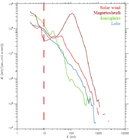
The solar wind pressure compresses the internal magnetic field lines on the dayside, distorting and confining them inside a magnetospheric cavity. As the solar wind is supersonic, this encounter creates a shock upstream the planet, called the bow shock. The solar wind is then slowed down and reaches a subsonic speed in a region called the magnetosheath. The magnetosheath acts like a buffer region between the interplanetary medium where the solar wind plasma is dominant and the near planetary environment where the planetary plasma is dominant. Hence, this transition region is filled with shocked, deflected, heated and high density solar wind plasma with its draped, frozen-in magnetic field (the draping of the IMF is discussed in more details in section 1.3.1.2)

As the solar wind is a conductive fluid, a current layer called the magnetopause exists to isolate the magnetic field of the planet from the IMF. The magnetopause is the outer boundary of what is called the magnetosphere, which is defined as the region of space where the magnetic field lines have at least one end connected to the source of the internal magnetic field.

Only a small amount of solar wind particles finally go through the magnetopause, particularly in the cusp regions, more or less sporadically.

Figure 3. Illustration of the general features of the interaction of the solar wind with the Earth magnetic field. Superimposed in dotted lines are the main features of the Mars-solar wind interaction. The sizes of the planets

have been normalized for the purpose of comparison [adapted from Luhmann et al., 1991].

Though on the dayside the planetary magnetic field lines are compressed by the solar wind pressure, on the nightside they are pinched into a long magnetotail. The magnetotail is composed of two lobes of opposite polarity, depending of the inner magnetic field polarity, and extending in the anti-solar direction. They are isolated from each other by a plasma sheet, at which the radial component of the magnetic field reverses.

 (2) Cometary and Moon-like interactions (Callisto, Moon, Phobos, comets, …) The bodies concerned in this category do not possess an internal magnetic field nor a consistent atmosphere (the active comets at small heliocentric distances being excluded from this category). In this case, the obstacle to the flow of the solar wind is an incompressible

conducting body, such as an iron core or a salt-water ocean. The solar wind particles then

absorbed. This creates a plasma-absorption wake left in the plasma behind the body, which is characteristic for this kind of interaction. At the same time, the IMF diffuses into the low conducting outer layers of the obstacle at a rapid rate, so that it is barely perturbed from its upstream orientation. Contrary to different configurations (such as the magnetospheres detailed previously), neither the magnetic field nor the particles accumulate on the dayside.

An illustration of this interaction at the Moon is presented on the left side of Figure 4, adapted from Luhmann et al., [2004]. We clearly see that the IMF is hardly affected by the passage of the obstacle but that a wake cavity is formed downstream. In the case of the Moon, there is no bow shock upstream the body because the diversion of the magnetic field occurs inside the absorbing body.

Figure 4. Illustration of two different interactions of the solar wind with unmagnetized obstacles. Left: the Moon interacts mainly with the solar wind plasma, while le IMF is hardly disturbed. Right: in the case

of Venus, the presence of a substantial ionosphere produces a relatively impenetrable obstacle. Adapted from [Luhmann et al., 2004].

 (3) Induced-magnetospheres (Titan, Venus, Mars)

This class of interaction contains bodies that do not possess an intrinsic magnetic field at large scale but that possess a dense atmosphere. The word ‘induced’ used here refers to the general processes of creating an effective magnetic obstacle through plasma interactions [Luhmann et al., 2004]. The induced magnetic fields include the field perturbations resulting from electromagnetic induction, but also from the flow interaction.

In this case, the atmosphere of the bodies is partially ionized by the ultraviolet solar photons which create an ionosphere (see section 1.2.1.1 for more details). The obstacle to the solar wind is then an electrically conducting, compressible ionospheric shell which balances

the external plasma pressure at a boundary generally called ionopause. As in the case of the magnetospheres, the solar wind slows down upstream the obstacle and becomes subsonic when it crosses the bow shock upstream the body. At the same time, the interplanetary magnetic field lines pile up in front of the obstacle and drape around it, as shown on the right side of Figure 4 for the case of Venus. The so-formed induced magnetosphere also includes a magnetosheath and an induced tail which is essentially the extension of the magnetosheath into the wake.

In Figure 5 is shown a simplified scenario of the creation of an induced magnetosphere. The intrinsic neutral environment of a planet (step 1) is ionized through different processes by the ultraviolet solar photons (step 2). The so-formed ionosphere is a conductor (step 3). The incoming magnetic fields generate induced currents in the ionosphere that keep the IMF from penetrating through the body by generating a canceling field (step 4). This situation persists as long as the external magnetic field keeps changing its orientation and/or magnitude [Luhmann, 1995].

Figure 5. Illustration of the steps leading to the formation of an ionospheric obstacle in the solar wind flow. Adapted from Kivelson and Russel [1995].

The induced magnetosphere interaction will be discussed in more details in section 1.3.1, for the specific case of Mars.

 (4) Mini-magnetospheres (Ganymede, Mercury, Moon magnetic anomalies)

This last class gathers bodies with no significant atmosphere but with a magnetic field (intrinsic or remnant) two or three orders of magnitude weaker than in the magnetosphere class. This class appears like an intermediate case between bodies with low or no magnetic field and planets with strong intrinsic magnetic fields.

The solar wind plasma directly interacts with the surface of the body, as for the Moon, since no atmosphere can shield it. This interaction contributes to the creation of a thin atmosphere: an exosphere (see section 1.2.1.1), whose composition reflects the composition of the surface. In the case of Mercury, other processes like thermal desorption and meteorit bombing are also to be considered. The low gravity of the planet added to its high surface temperature due to its vicinity to the Sun facilitate the creation of such an exosphere.

In addition, there is a magnetosphere-like interaction with the formation of a magnetosphere, a magnetopause, cusps, a magnetotail, etc. However, there is no coupling with an ionosphere, with no creation of ionospheric currents like at Earth, but there is a coupling with the core. An illustration of the magnetosphere of Mercury is given in Figure 6.

Much remains to be discovered about these types of magnetospheres, and future missions, such as Bepi-Colombo at Mercury or JUICE at Ganymede, will help understanding this kind of interaction.

As observed in Figure 2, the Martian interaction with the solar wind cannot be restricted to one category, due to its magnetic and atmospheric history. The global interaction can be similar in some extent to that of induced magnetospheres, such as Venus or Titan, but the presence of strong crustal magnetic sources induces localized mini-magnetospheres. Understanding the Martian interaction with the Sun hence begins by understanding the nature of the Martian obstacle. The current atmospheric and magnetic environment of Mars are described respectively in section 1.2.1.1 and 1.2.1.2. We then propose in section 1.2.2 an overview of the Martian history, which enables a better understanding of the current observations. This finally leads us to the description of the Martian interaction with the solar wind in section 1.3.

1.2.

The Martian obstacle

Mars is the fourth planet of our solar system and the last telluric one. It orbits around the Sun on an elliptic orbit with a maximum distance to the Sun (aphelion) of 1.67 AU and a minimum distance to the Sun (perihelion) of 1.38 AU, which imply an eccentricity of 0.0935, much higher than the Earth one (0.0167). Mars inclination on its orbital plane is 25,19°, which is comparable to the Earth (23,44°) and implies the presence of seasons.

The length of the day on Mars is quite comparable to the Earth one: ~24h37min, and the planet makes a revolution around the Sun in ~687 days, a little less than two Earth years. With an average radius of 3386,2 𝑘𝑚, Mars is twice as small as the Earth and the gravity at its surface is three times smaller. The temperature at its surface can vary from -3°C to -133°C.

1.2.1.

Mars today

Mars has been visited by more than twenty spacecraft - landers - rovers to date (see section 2.1 for more details). These in-situ measurements have allowed a better knowledge of the Martian object, its current atmosphere (1.2.1.1) and magnetic field (1.2.1.2), which both are important to understand the interaction of Mars with the Solar wind.

1.2.1.1. Atmosphere - Exosphere - Ionosphere: who is who?

Atmosphere

Based on the nomenclature used for the terrestrial atmosphere, the Martian atmosphere can be divided into several layers according to the mechanisms involved (turbulence, molecular diffusion, photoionization, heating by absorption of UV rays). Taking the collisional point of view, the atmosphere can be divided into two parts: the barosphere and the exosphere (Figure 7). These two layers are characterized by a dimensionless number, the Knudsen number (Kn):

Kn = 𝜆 𝐻

The mean free path λ can be defined as follows, in the case of a gas composed of a single species, where n is the density of the species, and 𝜋𝜎2 _{the cross section :}

𝜆 = 1 𝜋𝑛𝜎2_√2

The scale height H — corresponding in every point to the altitude to be raised for the pressure to be decreased by a factor of 𝑒 — can be defined as follows:

𝐻 =𝑘𝐵𝑇 𝑀𝑔

Where M is the mean molecular mass, g the local acceleration of gravity, 𝑘_𝐵 the Boltzmann constant and T the medium temperature.

Figure 7. Altitudinal extension of the different atmospheric regions and boundaries discussed in section 1.2.1.1 and of the ionosphere.

Regarding the Knudsen number, the barosphere and the exosphere can be defined as follows:

 The barosphere is a region of low Knudsen number (𝐾𝑛 ≪ 1). This is the inner part of the atmosphere, with the highest density. The dynamics is dominated by collisions between molecules and atoms, which result in a collisional medium, dominated by diffusion processes.

 The exosphere is a region of high Knudsen number (𝐾𝑛 ≫ 1). It corresponds to the external layer of the atmosphere and hence the less dense. The dynamics is here dominated by external forces, especially gravitation. It is characterized by a very high Knudsen number, which means that there are very few collisions, and that the trajectories of the particles are essentially ballistic. The exosphere is an exchange area between the lower atmosphere and the interplanetary medium.

The transition between the collisional and non-collisional medium is called the exobase. It has been estimated at 250 km by Anderson and Hord [1971], after Mariner 6 and 7 observations.

The barosphere can be divided into two layers, regarding the mixing of the atmospheric components: the homosphere and thermosphere (see Figure 7). The homosphere and thermosphere are separated by a layer called the homopause (located at ~125 km mean altitude on the dayside).

 The homosphere is the lower layer, characterized by atomic and molecular constituents which are well mixed by winds and dissipative turbulence [Stewart, 1987; Bougher 1995;

Bougher et al., 2000; 2009; 2014]. The relative proportion of each species stays quasi-constant, no matter the molecular mass.

 The thermosphere corresponds to the region where the atomic/molecular diffusion dominates. Individual species begin to separate according to their unique masses and scale heights. The low mass species have higher scale height and will then be more abundant at higher altitude regarding heavier species whose density will decrease more quickly with altitude. The first in situ measurements of the thermosphere composition were obtained by the Viking 1 and 2 entry probes in 1976 [Nier and McElroy, 1976; Nier et al., 1976]. The measurements recorded along the descent of the landers highlighted the presence of CO₂, N₂, Ar40 _{, O}

2, NO and maybe CO in the Martian atmosphere.

More recently, measurements made with the Mars Atmosphere and Volatile EvolutioN (MAVEN) spacecraft down to the homopause improved our knowledge of the composition of the atmosphere and its variation with altitude. On the left panel of Figure 8 is plotted the neutral composition obtained during one orbit down to 133,8 km, near the equator at noon, and on the right panel is plotted the average vertical neutral profiles obtained at 45° solar zenith angle [Mahaffy et al., 2015b]. We clearly observe that the lower atmosphere is dominated by 𝐂𝐎_𝟐 whereas the higher atmosphere is dominated by O, with significant amount of O2, N2 and N.

Figure 8. Neutral profiles obtained with the NGIMS instrument on MAVEN [Mahaffy et al., 2015]. Left panel: an example of the variation with altitude of nine atomic and molecular species during a passage down to 133.8 km. Right panel: the average vertical profiles for nine upper atmosphere species at 45° solar

zenith angle.

Ionosphere

The upper neutral atmospheric region includes the thermosphere and the exosphere (also sometimes referred to as the corona). The upper neutral atmosphere interacts directly with the solar wind particles and photons, modifying the plasma neighboring the planet and creating an

ionosphere (i.e. a part of the atmosphere that is ionized). While the thermosphere extends from

~100 to ~250 km altitude, the ionosphere can extend from ~100 to ~400 km altitude [Bougher et al., 2014].

The process of ionization involving photons is called photoionization, and the process involving energetic-particles is often called impact ionization. While photons mainly come from the Sun, the ionizing particles can come from the Sun, but also from the galaxy (cosmic rays), or from the ionosphere itself. The only requirement for the photons and energetic particles to ionize the neutral atmosphere is that their energy exceed the ionization potential or binding energy of a neutral. Atmospheric ionization is usually attributable to a mixture of these various sources, but one often dominates.

The three predominant ionization processes at Mars are the following (but there are several other mechanisms which play an important role in the dynamics and the escape of the ionosphere, see section 1.2.2.2):

 Photoionization:

Solar photons arriving on Mars mainly interact with O and CO₂ by the following mechanisms:

CO₂+ hν → CO₂+_{+ e}−

O + hν → O+_{+ e}−

These two reactions are both associated with an ionization threshold near 90 𝑛𝑚: 91,1 𝑛𝑚 for oxygen and 89,9 𝑛𝑚 for carbon dioxide. This means that only photons with lower wavelengths can photoionize O and CO₂. This corresponds to solar photons in the “extreme” ultra-violet (EUV) and ultraviolet (UV) wavelength ranges. Photoionization is the most important ionization process at Mars, in particular to create the dayside ionosphere.

 Ionization by electronic impact:

It corresponds to the interaction of electrons coming from the solar wind or the magnetosheath with the atmospheric neutrals thus producing ions. This process is the dominant ionization process producing the nightside ionosphere. Following is an example of such ionization by electronic impact with a neutral (M):

e−_{+ M → M}+_{+ e}−_{+ e}−

 Charge exchange reactions

The plasma of the solar wind or of the induced magnetosphere interacts with the neutrals of the atmosphere. The incident ions can extract an electron from the atmospheric neutrals and transfer them their positive charge, thus producing a new ion and an energetic neutral atom. This process plays an important role in the production of ions (and associated cyclotron waves) at high altitudes in the Martian corona, due to the solar wind incident protons. Following is an example of such charge exchange reaction:

H+_{+ O → O}+_{+ H}

In Figure 9 are plotted the altitude profiles of the main ions of the Martian ionosphere, obtained by Benna et al., [2015] during the first eight months of the MAVEN mission in

2014-2015. We can observe that the dominant ion is O₂+ _{below 300 km, with a smaller but significant}

amount of O+ _{and CO} 2

+_{, depending on the altitude.}

Figure 9. Altitude profiles of the averaged density of ionospheric ions measured by NGIMS onboard MAVEN. Measurements were made at a solar zenith angle of 60° and at altitudes between 150 and 500 km. The vertical

profile of the total ion density 𝑁_𝑖 is also plotted in black. [Benna et al., 2015]

The altitude profile of ion production shows a peak at some altitude (the so-called Chapman layer), because the rate of ionization depends on both the neutral density (which decreases with altitude) and the incoming solar photons or precipitating plasma intensity (which decreases towards the surface due to absorption by the atmosphere). The altitude of this peak is specific to each ionization source. Hence, we usually observe three peaks on the Martian ionospheric profiles on the dayside: one for the EUV-UV, one for the X-ray and one for the meteoroids. Those peaks are different on the nightside.

1.2.1.2. The Martian magnetic field

The question of the Martian intrinsic magnetic field remained unanswered until the end of the 90s, when it was proved that, at the present time, Mars does not possess any global

magnetic field generated by an internal dynamo.

The first observations of the Martian magnetic field in the near Martian environment had been made by the Mariner 4 spacecraft in 1965 when it passed within 13 200 km of the planet.

The lack of detectable magnetic field signature attributable to Mars led to the conclusion that the Martian magnetic moment could not exceed 3 × 10−4 that of the Earth dipole moment, equivalent to an equatorial field of less than 100 nT [Smith et al., 1965]. Additional measurements were made by Mars 2, 3 and 5 in the early 1970s and by Phobos 2 in 1989. Even the Phobos 2 spacecraft, whose lowest altitudes were at 850 km from the surface, did not measure any magnetic field providing evidence of an intrinsic magnetic field. The scientific community was then divided between those claiming the presence of a small intrinsic dipole moment [Dolginov and Zhuzgov, 1991; Slavin et al., 1991; Verigin et al., 1991a; Möhlmann et al., 1991] and those claiming the absence of any intrinsic magnetic field [Russell et al., 1995;

Gringauz et al., 1993].

Mars Global Surveyor (MGS) was the first spacecraft to obtain magnetic field observations beneath the ionosphere (~170 to 200 km) in 1997-1998. It provided 83 periapsis passes with altitudes between 100 and 170 km. This region is particularly interesting since it is shielded from the confounding effects of the solar wind interaction with the Martian atmosphere and ionosphere. The induced magnetic fields resulting from this interaction can indeed reach levels similar to those arising from a planetary field of internal origin (see section 1.3.1.3).

Acuña et al. [1998] showed that on several orbits reaching the underside of the ionosphere, relatively weak magnetic fields (≤ 5𝑛𝑇) were observed. They hence conclude that Mars does not possess a global intrinsic magnetic field on a large scale, and therefore no dynamo at present.

However, on some other orbits, like the one presented in Figure 10, the magnetometer recorded large magnetic fields near the periapsis. The amplitude of the magnetic field plotted on the right panel is projected on the MGS orbit on the left panel, so that the highest amplitude of the magnetic field (~400 nT) is observed at the closest point of the spacecraft orbit, while no significant magnetic field can be observed on the remaining part of the orbit. For these kind of orbits, it was found that the observed magnetic fields were restricted to a segment of the spacecraft trajectory that passed close to the Martian crust. Hence, the observed magnetic signatures are not of global scale, as it would necessarily be if they were generated in the deep interior, for example by a dynamo. It was thus discovered that the magnetic field of Mars is dominated by intensely magnetized sources, distributed non-randomly in its crust [Acuña et al., 1998, 1999].

Figure 10. Illustration of the magnetic field measured by MGS [Acuña et al., 1998].

Left panel: projection of the MGS spacecraft trajectory and observed magnetic field onto a plane perpendicular to the Mars orbit plane and the Mars-Sun line for a specific periapsis. The field observed along the trajectory at 3-s intervals is represented by a scaled vector projection of B originating from the position of the spacecraft at

such times. Field vectors are scaled to 400 𝑛𝑇 = 1 𝑅𝑀𝑎𝑟𝑠. Right panel: magnitude of the observed magnetic

field as a function of time for the time interval represented on the left panel.

Compiling the data obtained by MGS during two full Martian years at its 400 km-mapping altitude, Connerney et al., [2005] presented a global map of the magnetic fields due to remnant magnetism in the Martian crust. Figure 11 is an updated version of this map [Connerney et al., 2015]. It is a global map of the filtered radial magnetic field (∆𝐵_𝑟), color contoured over two orders of magnitude variation in signal amplitude. The map is superimposed on the Mars Orbiter Laser Altimeter shaded topography map.

The crustal magnetic sources, mainly located in the southern hemisphere, can be considered as small dipoles located under the Martian crust. They form closed magnetic field loops (see section 1.3.2.1), which extends beyond 120 km altitude over 70% of the surface, and can extend up to 1500 km altitude over the strongest southern sources. The crustal magnetic field can reach intensities exceeding 200 nT at 400 km in the southern hemisphere [Acuña et al., 2001]. The largest crustal magnetic field strength ever measured at Mars is ~1600 nT near 100 km altitude. This value can be compared to the typical strength of the Earth’s global magnetic field and magnetic anomalies measured at 400 km: 26000 nT and 10 nT, respectively.

Figure 11. Map of the remnant magnetic field of Mars observed by MGS at its nominal altitude of 400 km. Each pixel is colored according to the median value of the filtered radial magnetic field component observed within the ½° by ½° latitude/longitude range represented by the pixel. Contours of constant elevation (-4, -2, 0,

2, 4 km elevation) are superimposed (after Connerney et al., 2005).

The Martian obstacle to the Sun is then composed of the ionosphere, together with the

crustal magnetic sources. Both form magnetic fields that divert the incoming plasma around

the planet. Crustal magnetic fields contribute to the deflection in some regions of Mars (mainly in the Southern hemisphere), creating ‘mini-magnetospheres’. In other regions, the IMF carried by the solar wind induces currents (via Faraday’s Law) in the conducting ionosphere that generate magnetic fields (via Ampere’s Law). The shielding magnetic fields then deflect solar wind particles around the obstacle (via the Lorentz’s law).

The interaction of Mars with the Sun will be extensively discussed in section 1.3, after a brief incursion into the Martian history.