Robust prediction of dense gas flows under uncertain thermodynamic models

Science Arts & Métiers (SAM)

is an open access repository that collects the work of Arts et Métiers Institute of

Technology researchers and makes it freely available over the web where possible.

This is an author-deposited version published in:

https://sam.ensam.eu

Handle ID: .

http://hdl.handle.net/10985/15563

To cite this version :

Xavier MERLE, Paola CINNELLA - Robust prediction of dense gas flows under uncertain

thermodynamic models - Reliability Engineering & System Safety - Vol. 183, p.400-421 - 2019

Any correspondence concerning this service should be sent to the repository

Administrator :

archiveouverte@ensam.eu

Robust prediction of dense gas flows under uncertain thermodynamic

models

X. Merle

_{, P. Cinnella}

DynFluid Laboratory, Arts et Métiers ParisTech, 151 boulevard de l’Hôpital, Paris, 75013, France

A B S T R A C T

A Bayesian approach is developed to quantify uncertainties associated with the thermodynamic models used for the simulation of dense gas flows, i.e. flows of gases characterized by complex molecules of moderate to high molecular weight, in thermodynamic conditions of the general order of magnitude of the liquid/vapor critical point. The thermodynamic behaviour of dense gases can be modelled through equations of state with various mathematical structures, all involving a set of material-dependent coefficients. For several organic fluids of industrial interest abundant and high-quality thermodynamic data required to specify such coefficients are hardly available, leading to undetermined levels of uncertainty of the equation output. Additionally, the best choice for the kind of equation of state (mathe-matical form) to be used is not always easy to determine and it is often based on expert opinion. In other terms, equations of state introduce both parametric and model-form uncertainties, which need to be quantified to make reliable predictions of the flow field. In this paper we propose a statistical inference methodology for estimating both kinds of uncertainties simultaneously. Our approach consists of a calibration step and a prediction step. The former allows to infer on the parameters to be input to the equation of state, based on the observation of aerodynamic quantities like pressure measurements at some locations in the dense gas flow. The subsequent prediction step allows to predict unobserved flow configurations based on the inferred posterior distributions of the coefficients. Model-form uncertainties are incorporated in the prediction step by using a Bayesian model averaging (BMA) approach. This consists in constructing an average of the predictions of various competing models weighted by the posterior model probabilities. Bayesian averaging also provides a useful tool for making robust predictions from a set of alternative calibration scenarios (Bayesian model-scenario averaging or BMSA). The proposed methodology is assessed for a class of dense gas flows, namely transonic flows around an isolated airfoil, at various free-stream thermodynamic conditions in the dense-gas region.

1. Introduction

Flows of dense gases, i.e. flows of organic fluids of moderate to high molecular weight working close to saturation conditions, are en-countered in several engineering problems, one of the most attractive applications being represented by energy conversion cycles, like

heat-pumps, refrigeration and, most of all, Organic Rankine Cycles[1–5].

Dense gas flow simulations can be extremely sensitive to the model used to describe the fluid thermodynamic behavior and its closure

coefficients[6], i.e. to the equations of state (EOS). Specifically, EOS

give raise to two kinds of uncertainties: the first one concerns choosing a suitable mathematical form among the many available (e.g., cubic EOS[7–9], virial EOS with a more or less large number of expansion

terms[10,11], reference EOS based on power-law expansions of the

Helmoltz free energy[12]); on the other hand, the material-dependent

coefficients associated to the EOS are often imperfectly known, espe-cially for complex organic fluids for which abundant high quality data are less readily available than for widely employed light gases like

hydrogen, nitrogen, carbon dioxide, etc [13]. Although parametric

uncertainty may be critical for the accurate prediction of dense gas

flows, in[6]it was shown that for some complex gases the model-form

uncertainty can be even overwhelming with respect to the former one. Several studies have addressed the problem of calibrating EOS from thermodynamic data available for the fluid(s) of interest. This can be

done either in a deterministic way (e.g. [13] and references cited

therein) or stochastically, e.g. by using statistical inference

methodol-ogies [14,15]. In a previous work [16], the present authors used

aerodynamic data instead of thermodynamic ones for calibrating the material-dependent coefficients of equations of state (EOS) used to model the thermodynamic behavior of the working fluid. For that purpose, a Bayesian statistical procedure was used to infer on the posterior probability distributions of the closure coefficients associated with three well-known thermodynamic models, given data on the wall pressure distribution for a dense gas flow past an airfoil. The statistical model used for the calibration accounted both for uncertainties in the observed data and in the model form. The latter expresses the fact that, due to the simplifying assumptions intrinsic to any mathematical model of a physical system, this can never predict exactly the observed values,

even assuming that the best possible coefficients are available (see[17]

for a thorough discussion on the role of model-form uncertainties). The model-form uncertainty was represented as a Gaussian random vector with a given correlation structure, whose coefficients (called the

⁎_{Corresponding author.}

E-mail addresses:xavier.merle@ensam.eu(X. Merle),paola.cinnella@ensam.eu(P. Cinnella).

hyperparameters) were calibrated alongside the physical model para-meters.

Accounting for model-form uncertainty in the statistical calibration

is useful to temperate overfitting problems (see[16,18]). Nevertheless,

such problems are not completely avoided and the closure parameter posterior distributions have limited validity when used to predict flow configurations far away the one on which they where calibrated. In

other terms, they have no universal validity [17]. Additionally, the

model-form uncertainty term is specific to the kind of data used for the calibration and cannot be used, e.g., to predict a different quantity of interest (QoI) for a new flow.

A coherent framework for making predictions in situations where multiple competing models are available is represented by multi-model approaches, used in a plethora of applications including oil price pre-dictions, meteorology, ground-water modeling, aerodynamics, and

aeroelasticity [19–26]. Bayesian model averaging (BMA) [19,27] is

among the most widely used multi-model approaches, where posterior average predictions are inferred by weighing individual forecasts from competing models based on their relative skill, with predictions from better performing models receiving higher weights than those of worse performing models. BMA avoids having to choose a model over the others and provides instead a measure of the model-form uncertainty based on the level of agreement among the competing models con-sidered in the average. Due to the high computational cost when combined with complex computer models, BMA has found application in computational fluid dynamics problems, governed by complex

non-linear equations, only recently. In[28]a BMA approach was used to

investigate model-form uncertainty due to the existence of several competing closure models for the Reynolds-Averaged Navier–Stokes (RANS) equations, often used to describe turbulent flows. More speci-fically, an extended formulation of BMA was adopted (first suggested in

[19], see also[24]for an application to ground-water modeling), which

accounts also for the uncertainty about the validity of the calibrated model parameters when applied to a new prediction scenario. Such an

extension, termed Bayesian Model-Scenario Averaging (BMSA) in[28],

amounts to considering each realization of a model supplemented by coefficients adjusted on different calibration scenarios as a component of the mixture, weighted through a suitable ’scenario’ probability. In this framework, the posterior predictive distribution of a QoI for a model applied to a new scenario is the weighted average of the pre-dictions of a model using different sets of coefficients. An attractive feature of BMSA is that, if new sets of coefficients become available, these can easily be added to the BMSA mixture, which is then expanded to a larger set of scenarios. Differently from BMA, where the model weights are inferred during the calibration process, in BMSA the sce-nario weights have to be chosen a priori, according to expert judgement or Bayesian criteria. Eventually, if data are available for the new sce-nario, these can be used to infer on the scenario weights. This is how-ever not the case in general, so that a key point is to find a suitable a priori criterion for choosing the scenario weights. An empirical cri-terion, based on the level of agreement among the competing models

calibrated on the same scenario, was proposed in[28]and successfully

applied to the prediction of a variety of turbulent perfect gas flows in [28,29].

Accounting for calibration scenario uncertainty is an essential fea-ture for dense gas flows, which are very sensitive to the thermodynamic

operating conditions (see, e.g.,[30]). A standard approach to calibrate

a model over data sets coming from different scenarios consists in in-ferring from all data sets simultaneously. For instance, Cheung et al.

[18]. inferred on the coefficients of a turbulence model using velocity

and skin friction data for flat plate boundary layers subject to three different external pressure gradients. In such an approach, the resulting coefficients represent a compromise allowing the model to fit reason-ably well all of the available data. The calibration procedure can than be applied to different models, and a final BMA can be used to predict a

new case while accounting for model-form uncertainty. The interest of such an approach is that it avoids choosing scenario weights. The drawback is that the likelihood function involved in the inference of such a large data set is a multivariate random function, with a high-dimensional correlation matrix that may be hard to build and invert. Additionally, including new data sets implies restarting the calibration from scratch. For this reason, in this paper we propose an alternative approach, termed Bayesian Scenario Averaging (BSA). This can be seen as a special case of BMSA, where a single model is calibrated against several competing scenarios and applied to a new one. A suitable a priori criterion is proposed to weight the scenarios. BSA is assessed against the standard approach in the case of dense gas flow predictions. The main goal of the present work is to develop a robust tool for prediction of dense gas flows with quantified thermodynamic un-certainties, based on Bayesian inference and model averaging. Specifically, we first use Bayesian calibration for updating the coeffi-cients of two different EOS, namely the cubic EOS of

Peng-Robinson-Strjyek-Vera[9](PRSV) and the 5th-order virial Martin-Hou EOS[10]

(MAH). For that purpose, similarly to[16], we consider pressure data

for dense gas flows past an airfoil[31–33]characterized by different

free-stream thermodynamic conditions. For all the flows, the airfoil geometry and the free-stream Mach number are the same, while the free-stream pressure and temperature may vary, leading to a different thermodynamic behaviour. In this context, we term a scenario a given choice of the operating thermodynamic conditions. The EOS are cali-brated versus different scenarios individually or simultaneously. In the first case (called single-point calibration), posteriors of the coefficients resulting from different calibrations are propagated through a new scenario by means of BSA. The advantages of the BSA approach and the role of the weighting criterion are discussed for two prediction sce-narios (not used for calibration) for which validation data is available. Finally, information from different scenarios and models is mixed to-gether using BMSA, demonstrating the importance of accounting for both parametric and model-form uncertainty.

The paper is organized as follows: inSection 2 we present the

physical problem, the governing equations and the thermodynamic models (EOS), and we briefly describe the numerical solver used for the

computations. InSection 3we describe the data used for the

calibra-tions and the choice of the calibration and prediction scenarios. Section 4 illustrates the Bayesian calibration methodology and the BMSA framework for robust prediction. Numerical applications of the calibration and prediction approach to transonic dense gas flows are reported inSections 5and6. Finally,Section 7is devoted to conclusions and perspectives.

2. Description of the problem

The objective of this study is twofold: (i) first we compare two ca-libration strategies to take into account data coming from multiple flow scenarios, (ii) we assess the capability of BMSA to provide robust pre-dictions of dense gas flows. Such flows are of special interest for energy conversion machines which involve an expander (often a turbine) and/ or a compressor, characterized by the presence of bladed disks, through which the dense gas flows. Since blade sections can be roughly seen as airfoils, hereafter we investigate the feasibility of our calibration methodology for a simplified configuration, roughly representative of a blade section, i.e. an isolated airfoil. Such kind of configuration was used in the past to investigate qualitatively dense gas effects in

turbo-machinery[34,35]. Moreover, for this simplified problem sensitivity

studies of the impact of thermodynamic uncertainties on flow simula-tion results where carried out in[6].

Precisely, the case selected for this study is the steady transonic flow of a dense gas over a thin wing section, namely, a NACA0012 airfoil. The working fluid is a siloxane (silicon oil), known with the commercial name of D5 (chemical formula ((CH3)2SiO)5).

2.1. Governing equations

For simplicity, the flow around the airfoil is assumed to be inviscid, which represents a good approximation as long as the QoI is re-presented by the wall pressure distribution and the flow boundary layer remains attached. This amounts to consider that the flow is governed by the compressible Euler equations, written hereafter in integral form for a control volume Ω with boundary ∂Ω:

+ =

w f n

d

dt d · dS 0 ₍₁₎

In Eq.(1), w is the conservative variable vector, where

=

w ( , v E, )T

n is the outer normal to ∂Ω, and f, is the flux density:

=

f ( , ¯,v I vv v, H)T

where ρ is the density, v is the velocity vector, E the specific total

en-ergy, = +H E p/ the specific total enthalpy, p is the pressure andI¯ is

the unit tensor. The preceding equations are completed by a thermal equation of state:

= w w

p p( ( ), ( ))T ₍₂₎

with T the total pressure, and by a caloric equation of state for the specific internal energy e, which must satisfy the compatibility relation:

= w w = + e e T e c T dT T p T p d ( ( ), ( )) ( ) T T v 0 , ₂ 0 0 (3)

In Eq. (3), cv, ∞ is the ideal gas specific heat at constant volume,

quantities with a prime superscript are auxiliary integration variables, and subscript 0 indicates a reference state. The caloric equation of state

is completely determined once a variation law for cv, ∞has been

spe-cified.

The problem setup is completed by specifying the free-stream con-ditions, i.e. flow Mach number and angle of attack and thermodynamic conditions at the far field. These are treated in the following as

de-terministic and equal toM =0.95andAoA=00_{for all cases. On the}

other hand, the free-stream thermodynamic conditions, given in terms

of reduced pressurepr, =p p/cand density r, = / ,c are used to

specify the different flow configurations, i.e. the scenarios.

For dense gases, advanced EOS are needed to account for their complex thermodynamic behaviour, which may be described by means

of the fundamental derivative of gas dynamics[36]

= + a

a

: 1

s (4)

where ρ is the fluid density, a the sound speed, and s the entropy. Γ can be interpreted as a measure of the rate of change of the sound speed with density in isentropic perturbations. If Γ < 1, the flow exhibits an uncommon sound speed variation in isentropic perturbations: a grows in isentropic expansions and decreases in isentropic compressions, the opposite of what happens in “common” fluids. For instance, in perfect

gases, Γ is equal to +( 1)/2,where the specific heats ratio γ is always

greater than 1 for thermodynamic stability reasons; therefore, Γ > 1 as well. Finally for some heavy polyatomic fluids, referred to as the Be-the–Zel’dovich–Thompson (BZT) fluids, Γ may take negative values in a small thermodynamic region above the liquid/vapor saturation curve, leading to non classical behaviors in the transonic and supersonic re-gime, such as expansion shock waves, mixed shock/fan waves, and

splitting shocks (see, e.g.[35]and references cited therein). The

ther-modynamic region in the vapour phase where Γ < 1 is often termed the dense gas region, while the vapor region where Γ < 0 is called the inversion zone. The presence of regions of low or negative values of the

fundamental derivative within a flow field may change dramatically the behaviour compared to that of a classical gas. This is why the size and location of the inversion zone has a deep impact on the resulting flow field. The inversion zone has been found to be extremely sensitive to the equation of state in use and the associated input parameters (see e.g. [6]).

In this work, we consider two alternative thermodynamic models for the thermal equation of state, namely, the

Peng-Robinson-Stryjek-Vera (PRSV) cubic equation of state [9], and the multi-parameter

Martin-Hou (MAH) equation[10], based on a five-term virial

expan-sion. Both models have been often used in the dense gas literature, see e.g.[6,16].

In addition to the preceding EOS, we also consider for calibration and validation purposes (as discussed later) a more complex and ac-curate thermodynamic model, namely, the multiparameter technical

equation of state introduced by Span and Wagner (SW) [12] with

coefficients adjusted to D5 in[37]. This is a complex technical equation

of state, which is considered as the most accurate and complete ther-modynamic model presently available for this fluid, provided that a sufficiently large set of high-quality experimental data is available for a reliable fitting of the model coefficients, i.e. for reproducing experi-mental data with very high accuracy. One drawback is that this EOS is much more costly than the preceding ones. In practice, the equation coefficients are obtained by means of a regression procedure: the ex-perimental data used for calibration are weighted in such a way that high-quality data contribute with higher weights. Experimental data with uncertainties larger than a required threshold are discarded, or, when no or insufficient data are available for a certain region, they are weighted according to their level of uncertainty. Note that, due to the limited and highly uncertain data available for the dense gas of interest, the SW model is in practice also affected by significant uncertainties, of the order of about 10%. In the following calibrations, these are treated as “observational” uncertainties.

The main features of the three models are briefly recalled hereafter.

We refer to[6],[16]for a discussion of their sensitivity to uncertain

thermodynamic input parameters.

2.2. Thermodynamic models PRSV model

The cubic Peng and Robinson equation of state with modifications

suggested by Stryjek and Vera[9]can be written, in reduced form (i.e.

with thermodynamic quantities normalised with respect to their values at the liquid/vapour thermodynamic critical point), as:

= + p T Z v b a T v b v b / ( ) 2 r r c r r r r r r r 2 2 ₍₅₎

where the subscript r denotes a reduced quantity,(•)r=(•)/(•) ,c the

subscript c denotes critical-point quantities, v the specific volume, and:

= = a T Z T b Z ( ) (0.457235/ ) ( ), 0.077796/ r r c r r c 2 (6) withZc=(p vc c)/(RTc)the critical compressibility factor and R the gas

constant. The function α(Tr) is an adimensional relationship depending

on the reduced temperature and the substance acentric factor ω:

= +

T m T

( )r [1 (1 r0.5)] ,2 (7)

with m as a function of the acentric factor ω

= + +

m 0.378893 1.4897153 0.17131848 2 0.0196554 3 ₍₈₎

The critical compressibility factor is unequivocally determined by im-posing that prequals 1 at the critical point, i.e. for =vr 1,Tr=1,which

leads to the solution of a cubic equation for Zcwith only one relevant

root ( =Zc 0.3112). Thus, the only free parameter left in the thermal

equation is the acentric factor ω.

contribution to the specific heat at constant volume, represented here by a power law of the form:

= c T c T T T ( ) ( ) v v c c n , , (9) where the c subscript denotes critical-point values, and the exponent n and the ideal-gas-limit isocoric specific heat at the critical temperature

cv, ∞(Tc) are material-dependent constants.

Finally, the non-dimensional PRSV model (5,9) depends on the

uncertain parameters ω, n, and cv, ∞(Tc).

MAH model

The comprehensive thermal equation of state of Martin and Hou

[10]reads: = + = p T Z v b f T v b ( ) ( ) ( ) r r c r r _i r i r r r i 2 5 , (10) with =br 1 _Zc/ 15, =20.533 31.883 ,Zc and = + + f_{r i},( )Tr Ar i, B Tr i r, Cr i, exp( kTr)

withk=5.475. The gas-dependent coefficients Ar, i, Br, i, Cr, ican be

expressed in terms of the critical temperature and pressure, the critical compressibility factor, the Boyle temperature (which may be expressed as a function of the critical temperature) and one point on the vapour pressure curve. The MAH equation of state is supplemented again by

Eq.(9)to compute the ideal gas contribution to the specific heat at

constant volume. Globally, the MAH thermodynamic model in reduced

form, Eqs. (10) and(9), requires the knowledge of six

material-de-pendent parameters, namely, the critical pressure pc, the critical

tem-perature Tc, the critical compressibility factor Zc, the normal boiling

temperature Tb, the exponent n and the reduced ideal-gas

constant-volume specific heat at the critical temperature cv, ∞(Tc). As a

con-sequence, we choose to neglect them for the following of the study. Nominal values of the different input parameters corresponding to D5

are given in Table1.

SW model

The last thermodynamic model considered in this study is a 12-parameter technical equation of state based on the functional form for

non polar fluids proposed by Span and Wagner ([12]). This is written as

an expression for the reduced Helmholtz free energy Φ (i.e. normalised with RTc), sum of an ideal-gas part, Φ0, function of the ideal-gas

iso-baric heat capacity cp, ∞, and by a residual term Φrthat takes into

ac-count real-gas corrections:

= + + + + + + + + + + + n n n n n n n n n n n n ( , ) exp( ) exp( ) exp( ) exp( ) exp( ) exp( ) exp( ) r 1 0.25 2 1.25 3 1.5 4 3 0.25 5 7 0.875 6 2.375 7 2 2.0 8 5 2.125 9 3.5 2 10 6.5 2 11 4 4.75 2 12 2 12.5 3 (11)

where n1, ... , n12are substance-specific coefficients, = /c is the

reduced density and = T Tc/ is the inverse of the reduced temperature.

Material-dependent coefficients for D5 have been taken from Ref[37].,

to which we refer for more details. The thermal and caloric EOS are

derived from the following thermodynamic relations:

= + = + p RT e RT 1 r ; 0 r

For the calculation of caloric properties, the SW EOS (Eq. (11)) is

supplemented by the ideal gas contribution to the specific heat at constant pressure, which is now approximated here as a polynomial function of the temperature:

= + = + + + c T R c T R c c T c T c T ( ) ( ) 1 p, r v, r 1 2 3 2 4 3 ₍₁₂₎

where the polynomial coefficients ci depend again on the substance

under consideration and are given for D5 in[37]. This model is

con-sidered as more accurate than the preceding ones. For this reason, it is used in the following to generate reference solutions used to calibrate the simpler PRSV and MAH models.

2.3. Numerical solver

Numerical solutions for the dense gas flow of interest are found by means of an in-house dense gas flow solver. The governing equations are discretized using a cell-centered finite volume scheme for structured multi-block meshes of nominal third-order accuracy, which allows computing flows governed by an arbitrary equation of state. We refer to

[38]and the references therein for more details about the numerical

solver and its validation.

Due to high computational cost, the dense gas solver is used to generate an inexpensive surrogate model, i.e. an analytical function providing an approximation of the code output for a given choice of the input parameters. The surrogate model used in this work is a determi-nistic piecewise polynomial interpolation. A more detailed description of the surrogate model, along with a discussion about the

approxima-tion error can be found in[16].

3. Calibration data

3.1. Pseudo-experiment

Despite many past efforts for carrying out experiments for dense gas

flows[39–41], no detailed experimental characterization of dense gas

flows is available yet. Very recently, preliminary results have been

presented for nozzle flows of the light siloxane MDM[42]. These

in-clude flow visualizations and a single pressure measurement at the geometrical nozzle throat. Other dense-gas facilities are under

devel-opment, e.g. [43], so that a more complete body of experimental

knowledge will come into availability in the near future. In this work, to provide a proof of concept of our predictive methodology, we generate synthetic ”experimental” data by running the dense gas solver with the most complex and accurate thermodynamic model, namely, the SW model.

This numerical experiments consists of transonic steady flows of

siloxane D5 past an NACA0012 airfoil withM =0.95,AoA=00_and

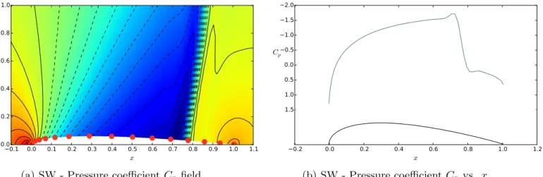
various choices of the free-stream thermodynamic conditions (corre-sponding to different scenarios), which are discussed later. Values of the pressure coefficient:

=

C p p

U

p ₁

2 2 (13)

(where U∞ is the free-stream velocity) are collected at 17 locations

distributed along the airfoil upper wall (simulated pressure taps)

highlighted by red symbols inFig. 1(a)). A more complete description

of the pseudo-experimental setup can be found in[16]. InFig. 1(a) we

report also typical isoline of the pressure coefficient around the airfoil, showing that the flow is characterized by a shock wave on the rear part of the airfoil for the chosen Mach number, as well as a typical

Table 1

Nominal values of thermodynamic properties and parameters for D5.

Tc(K) 619.15 pc(atm) 11.45 Zc 0.286 Te(K) 484.1 ω 0.6658 cν, ∞(Tc)/R 76 n 0.5208

distribution of the pressure coefficient along the airfoil (Fig. 1(b)). The collected synthetic pressure data are perturbed by adding a Gaussian noise with zero mean and standard deviation equal to 10% of the nominal value to simulate the effect of experimental errors. This

kind of observational error model is often used in the literature[44].

The 10% value for the standard deviation was chosen based on pre-liminary investigations of the sensitivity of the Span Wagner

thermo-dynamic model to uncertainties in the caloric quantities[6]).

3.2. Choice of the calibration and prediction scenarios

Pseudo-experimental data are generated for three choices of the free-stream thermodynamic conditions close to the liquid/vapour sa-turation curve, where dense gas effects play a crucial role in the flow physics. Their locations in the Clapeyron p v diagram are depicted in Figure 2and the corresponding values of the reduced thermodynamic

conditions (numbered from 1 to 3) are given inTable 2. Furthermore,

pseudo-experimental data were also generated for two additional op-erating conditions, not used in the calibration process, corresponding to

conditions 4 and 5 inTable 2and reported with green symbols inFig. 2.

Such conditions are referred to as the prediction scenarios, and the corresponding data are used to validate the predictive model. In this figure we also report the saturation curve computed according to the reference SW model as well as the saturation curves predicted by the PRSV and MAH models with parameters set to their nominal values. In

all cases, the operating conditions are sufficiently far from the satura-tion curve to avoid the appearance of two-phase flow condisatura-tions in the calculation. We checked that this condition was satisfied also for the perturbed values of the parameters considered in the calibration and prediction procedures.

4. Bayesian methodology

4.1. Bayesian calibration

This section describes the statistical procedure used to calibrate the

closure parameters associated to the EOS described inSection 2.

We observe that a QoI y can be computed as an output of the model

M given a set of parameters n_{: To that aim, consider first a generic}

physical problem of the form:

Fig. 1. Typical reference solution and location of the numerical pressure taps.

Fig. 2. Representation in the Clapeyron diagram of the

operating points (scenarios for the free-stream ther-modynamic conditions) used in the

pseudo-experi-ments. SW reference ( ), PRSV ( ), MAH

( ). Red symbols connected by lines:

calibra-tion scenarios; green symbols: prediccalibra-tion scenarios. (For interpretation of the references to colour in this figure legend, the reader is referred to the web version of this article.)

Table 2

Numerical values: specific volume v, density ρ end pressure p.

Point v/vc ρ/ρc p/pc 1 1.60 0.625 0.970 2 2.00 0.500 0.950 3 2.10 0.476 0.900 4 1.90 0.526 0.940 5 1.84 0.543 0.933 404

=

y M ( ) (14)

Note that y may also depend on additional parameters (explanatory variables) that are considered as known and do not need to be cali-brated (for instance the free-stream conditions or the airfoil geometry). Such fixed parameters are not explicitly represented as an argument for

M.

In the Bayesian framework, the unknown parameter vector θ is treated as a random vector, characterised by means of its joint prob-ability density function (pdf), noted as f. Due to the uncertainty on θ, y is a dependent random vector.

The main goal of Bayesian calibration is to achieve new knowledge about θ by constructing an improved representation of its pdf, starting from some prior knowledge on θ and some observed data.

For this purpose, assuming that new amount of information is available and represented by a random vector of observed data

D N,_{the Bayes rule simply states that:}

= = = = f D D f D D f D D f ( | ) ( | ) ( ) ( ) (15) where:

•

•

observe D¯, a realisation of the random variable D, if θ is known exactly;

•

knowl-edge of θ given information about D;

•

ob-serveD¯for all the values of θ, and acts as a normalisation constant

so that Eq.(15)is shortly written:

= =

f( |D D) f D( D| ) ( ).f (16)

Calibration is based on comparisons between modelled and ob-served data. Thus, it is necessary to extract from all possible model outputs quantities corresponding to the observed data. Note that the calibrated model can subsequently be used to predict other QoI, i.e. the output vector y includes, but is not necessarily equal to D. In the

fol-lowing of this section we assume for simplicity that =y D. To make this

point appear in the former notation, we rewrite Eq.(16):

= =

f( |D D y, ) f D( D y| , ) ( ).f (17)

even if this notation is redundant.

For our concerns, the uncertain parameter vector θ is the set of closure parameters associated to a given EOS, y is a vector of outputs from the dense gas solver M (in our case, the computed pressures at the 17 locations for which data are available), and D is a random vector of observed data (i.e. the reference pressure values).

From Eq.(17), it appears that the distribution of the prior and the

likelihood have a strong influence on the posterior and have to be chosen carefully. A number of priors have been proposed and used in

the literature. Ref.[45]recommends using the improper uniform pdf if

no information is available on the coefficients in advance of observing

the data, and a maximum entropy prior[46]when information

con-cerning their mean, covariance or other generalized moments is avail-able. In the context of the present paper we only expect the uncertain parameters to be positive and finite, but we do not have reasons to enforce any preferential parameter range. This is why we chose for the priors non-informative uniform distributions:

f( ) ([ , ])a b ₍₁₈₎

where the interval [a, b] is taken large enough to ensure a good ex-ploration of the parameter space, while avoiding to include nonphysical values. The likelihood function is a statistical model describing the probability of observing the data for a given choice of the model parameters. It may include information both about the observational

error on the data and the model error, including the effect of surrogate modelling if needed. In the following, we use a likelihood function resulting from a multiplicative/additive error model, similar to that

used in[18]for calibrating the closure coefficients of turbulence model

from measured velocity profiles in a turbulent boundary layer. We refer

to[47],[18]and the references cited therein for more details about

possible choices for the construction of likelihood functions.

In this work, the model includes an additive error modelling ob-servational noise and a multiplicative term representative of the model inadequacy. First, the data D at a given location xialong the airfoil wall

are modelled as:

= +

D x( )i D x^ ( )i ei (19)

with

•

•

The observational errors,e ii, =1, …,N( =N 17being the number

of data) are taken here as independent and normally distributed with zero mean and a standard deviation equal to 10% of the observed value.

On the other hand, the true processD^is in general not exactly captured

by the model(14)– even with the best possible choice of the parameters

θ – because of inadequacies intrinsic to the simplifying assumption used

to mathematically modelling the physical phenomenon under study. In this work, we assume the true process to be equal to the model output y (xi, θ), multiplied by an error coefficient ηi:

=

D x^ ( )i iy x( , )i (20)

which takes into account the discrepancy between the simulation and the actual system. Note that the use of corrective multiplicative coef-ficients to account for model predictive deficiencies (safety factors) is

common engineering practice (see, e.g.[48]). The vector of

model-in-adequacy terms =( , , )1 … N is assumed to be well represented by a

correlated Gaussian model of the form: (1,KM)with

= K x x i j N ( ) exp ( ) 2 , 1 , M ij 2 i j 2 2 ₍₂₁₎

where xiand xjare two distinct observation abscissas separated by the

length scale α. The coefficients σ and α are supplementary parameters intrinsic to the statistical model (hyperparameters) and are calibrated along with the parameters of the physical model. Note that σ represents the magnitude of the model inadequacy and thus can be taken as an indicator of the accuracy of a given model. On the other hand, the model-inadequacy term is expected to reduce the risk of over-fitting the model parameters, by introducing additional degrees of freedom (see,

e.g.[17]for a discussion about the importance of model-inadequacy

terms in Bayesian calibration). The correlation kernel(21)is an

adap-tation of the Matérn model suggested by Kennedy and O’Hagan[47]

and it is an expression of the belief that the code has some degree of smoothness, so that errors at closeby observation points (within a length α) are correlated.

With the preceding assumptions, the product( i i iy)= …1, ,Nhappens to

follow a normal distribution with mean y and a covariance matrix de-fined by:

=

K y y K i j N

( M ij) i j( M ij) , 1 , (22)

Finally, because( )ei i= …1, ,N is also a random vector, the likelihood

can be written under the form:

= f D y K D y K D y ( | , ) 1 (2 ) | | exp 1 2( ) ( ) N T 1 (23)

where =K Ke+K ,M with Kea diagonal matrix associated to the

An interesting point of the Bayesian framework is the possibility to account for various calibration scenarios in a one shot procedure by

considering a meta vector of data made of several D¯j. In such a

con-figuration, the covariance matrix KMmust be carefully modified to

consider the correlations, not only between the pressure taps within a particular scenario, but also between scenarios. In this work, the cov-ariance matrix accounts for correlations between pressure predictions for different scenarios. As such, considering J different scenarios, KMis

now written = + = + = + × K x x p p v v i j N k l J s k N i t l N j s t J N ( ) exp ( ) 2 exp ( ) ( ) 2 , with 1 , 1 , and ( 1) ( 1) 1 , M st 2 i j k l k l 2 2 2 2 2 (24) where p and v are the pressure and the specific volume and define a point of operating conditions in Clapeyron’s diagram; β is a new hyper parameter corresponding to a correlation length in Clapeyron’s dia-gram. Such a Bayesian inference is now referred as multi-point cali-bration, in contrast with single-point calibrations where only data from a single scenario are used.

From a numerical point of view, the inference is done by drawing samples from the prior pdf and the likelihood. For this purpose, we use a Markov-Chain Monte-Carlo (MCMC) sampler, based on the Metropolis-Hastings algorithm, which is well suited to represent non-classical pdfs. Precisely we use the implementation made available through the widely

used pymc1_{python library. Details of the Metropolis-Hastings MCMC}

algorithm can be found in the user guide.

Typically, a large number of samples is required to converge the posterior distributions. The results presented hereafter were obtained

by running samples from 106_{to 10}7_{draws, with a thin factor between}

10 and 20, and a burn-in of about 50%. To check that the convergence

is reached, we use the z-score method proposed by Geweke [49]

available in the pymc package. It consists of comparing the mean and the variance of segments from the beginning and the end of the Markov chain: = + z E[ ] E[ ] Var[ ] Var[ ] beginning end beginning end (25)

This z-score is theoretically distributed as standard normal variate. It is thus a statistical tool based on the hypothesis that

=

E[ beginning] E[end]. The point is that if this z-score falls within 2 standard deviations of zero, we cannot reject this hypothesis with 95% chance to be right. Along with this Geweke z-score, we also check for convergence through the evolution of the means, the auto-correlations, the correlations, the traces and the pdfs.

4.2. Bayesian model-Scenario averaging (BMSA)

Let us now consider =i 1,…,Imodels, modelling the same physical

problem, involved in =j 1,…,J calibration scenarios ={ , , }S1 …SJ

characterised by J vectors of observed data ={ ¯ , , ¯ }D1 …DJ . For model i

under scenario j, we write the Bayesian rule as:

= = = = = = = = = = = = = = = = = = = = = = = f M M S S D D f D D M M S S f M M S S f D D M M S S f M M S S d f D D M M S S f M M S S f D D M M S S ( | , , ) ( | , , ) ( | , ) ( | , , ) ( | , ) ( | , , ) ( | , ) ( | , ) i i j j j i i j i i j j i i j i i j i j i i j i i j j i j (26) where the subscript i of θ means that the random vector of parameters depends on the model and M is a discrete random variable defined on a

subset ={ ,M1 …,MI}of all possible models. Consider now a QoI Δ

and a prediction scenario S . By means of the law of total

prob-abilities[19]we then write:

= = = = = = = = = = f S f S D D M M S S p M M D D S S p S S ( | , , , ) ( | , , , ) ( | , ) ( ) i I j J j i j i j j j 1 1 (27)

where p represents the probability mass function (pmf) of a discrete random variable and:

•

ob-tained by propagating in the code the posterior distribution of θi

calibrated under model i by using data from scenario j,

•

As a consequence, the mean and variance of Δ are:

= = = E[ | ,S , , ] E[ | ,S D M S p M D S p S, , ] ( | , ) ( ) i I j J j i j i j j j 1 1 (28)

where we omitted to mention M, D and S to simplify the notations. In the preceding equations:

•

represents the mean of Δ by taking into account all the possible

models M calibrated on the same scenario Sj ,

•

ap-plying again Bayes rule

= = p M D S p D M S p M S p D M S p M S ( | , ) ( | , ) ( | ) ( | , ) ( , ) i j j j i j i j i I j i j i j 1 (31)

where p(Mi|Sj) is a prior user-defined pmf and p D M S( ¯ | , )j i j is the

model evidence: V ar[∆|S0, Z, M, S] = I X i=1 J X j=1 V ar[∆|S0, Dj, Mi, Sj]p(Mi|Dj, Sj)p(Sj)    within-model, within-scenario variance + I X i=1 J X j=1 E[∆|S0, Dj, Mi, Sj] − E[∆|S0, Dj, M, Sj] ¢2 p(Mi|Dj, Sj)p(Sj)    between-models, within-scenario variance + J X j=1 E[∆|S0, Dj, M, Sj] − E[∆|S0, Z, M, S] ¢2 p(Sj)   between-scenarios variance (29)

=

p D M S( | , )j i j f D( | ,j i M S fi, ) ( | , )j iM S di j ₍₃₂₎

The prior model mass function is chosen equal to:

= p M S

I

( | )i j 1 ₍₃₃₎

meaning that all models have the same prior probability before

obser-ving data. Finally we chose the prior scenario mass function as in[28]:

= = = ₌ = p S S E S D M S E S D S ( ) (a) [ | , , , ] [ | , , , ] (b) j j i I j i j j j 1 / 1 / 1 2 j p j J j p 1 (34)

where ϵjin Eq. (34b) is a measure of the dispersion of different model

predictions for scenario S′ using coefficients calibrated under scenario

Sj.

A special subclass of BMSA problems arises when there exists only one model. The BMSA equations are simplified and reduced to

= = E[ | ,S , ] E[ | ,S D S p S, ] ( ) j J j j j 1 (35) = + = = Var S Var S D S p S E S D S E S p S [ | , , ] [ | , , ] ( ) within-scenario variance ( [ | , , ] [ | , , ]) ( ) between-scenarios variance j J j j j j J j j j 1 1 2 (36) and such problems will now be referred as Bayesian Scenario Averaging (BSA). In this case the scenario pmf (34a) cannot be used any more. We suggest instead the following formulation:

= = = = = + = = = p S S E y D D S S D E D D S S ( ) (a) [ | , ] [ | , ] (b) j j j j j j j 1 / 1 / 2 j p j J j p 1 (37) where the first term of the right hand side represents the error between the posterior mean output calibration quantity y and the reference data

D¯ ,j and the second term stands for the model inadequacy.

5. Calibration results

In this section we apply the statistical calibration framework

de-scribed inSection 4.1to infer on the input coefficients of two

ther-modynamic models. As anticipated inSection 3.2, the data used for the

calibration are synthetic pressure measurements at 17 locations along

the airfoil wall. Previous sensitivity analyses[16]show that, for the

PRSV model, the most influential parameters are the acentric factor ω and the specific heat cv, ∞, with n having an almost negligible effect. For

MAH, only the critical temperature and pressure Tc, pc have a

sig-nificant influence on the model variance, while the effect of other parameters is rather negligible. Also note that the two parameters ex-hibit significant interactions (i.e. varying them jointly has a strong ef-fect on the variance) for flow cases with shock waves, due to the strong nonlinear effects characterizing the shock region. Such interactions have a strong impact on the calibration results, leading to posterior correlations of the calibrated parameters. Specifically, in our previous

work[16]a clear posterior correlation between ω and cv, ∞was

ob-served when calibrating the PRSV EOS. Similarly, a correlation between

Tcand pcwas observed for MAH. For this reason, in both cases we chose

to fix one of the correlated parameters. The acentric factor ω and the

critical pressure pc are then removed from the uncertain parameter

vector of the PRSV and MAH models, respectively, and kept fixed to their nominal values. For the remaining uncertain parameters and the hyperparameters we assumed large non-informative prior distributions,

given inTable 3, which encompass the nominal values. The upper and

lower bounds allow for a wide search of the parameter space, while avoiding physically inadmissible values (e.g., negative values or values leading to thermodynamic conditions lying in the twophase region -seeSection 3.2).

5.1. Results for the PRSV model

The results of the calibrations of the PRSV EOS against different sets

of data are reported inTable 4in terms of average and standard

de-viation of the posterior distributions obtained for the various scenarios. The calibration against the three data sets simultaneously (multiple-point calibration) is referred to as scenario “123” in the following. In all

cases the physical parametercv and the hyperparameter σ are well

informed from the data.

Concerning the posterior distributions of the PRSV parameter cv, ∞,

two tendencies are observed. For calibration scenarios 1 and 123 the

posterior mean of cv, ∞is close to 90.0, i.e. about 20% higher than the

nominal value. For scenarios 2 and 3 the mean is close to approximately 136. More generally, calibration scenarios 2 and 3 lead to similar posteriors for all the parameters and hyper parameters. This is mainly because the operating points 2 and 3 are closeby in the Clapeyron diagram and the corresponding pressure data are similar. In all cases,

calibration leads to extremely peaked posteriors for cv, ∞, whose

sup-port is much smaller than the prior distributions. This indicates that the computed posteriors are independent on the selected prior. The pos-terior mean of the hyper parameter σ is the smallest for scenario 2 (E [σ] ≈ 0.262) and the largest for point 1 (E[σ] ≈ 0.734). We recall that, in our statistical models for the likelihood based on Eq. (23) or Eq. (24)

Table 3

Prior distributions of physical and hyper parameters for the two EOS under investigation. PRSV MAH Tc – (550, 640) cν, ∞(Tc) (30, 400) – σ (0.0, 3.0) (0.0, 3.0) α (10 , 10 )5 5 _{(10 , 10 )}5 5 β (10 , 10 )5 5 _{(10 , 10 )}5 5 Table 4

PRSV model: mean E and standard deviation S of the posterior distributions of the parameters for the various scenarios.

Mean and Std. deviation Scenario j

1 2 3 123 E c[v, |Cp jref,,PRSV] 90.772 135.762 135.940 91.827 S c[v, |Cp jref,,PRSV] 0.247 6.013 4.026 0.555 E[ |C_{p j}ref_,,PRSV] 0.734 0.262 0.447 0.379 S[ |C_{p j}ref,PRSV] , 0.773 0.067 0.114 0.049 E[ |C_{p j}ref_,,PRSV] 50053.635 0.033 0.034 0.011 S[ |C_{p j}ref,PRSV] , 28912.708 0.016 0.013 0.003 E[ |C_{p j}ref_,,PRSV] – – – 0.123 S[ |C_{p j}ref,PRSV] , – – – 0.028

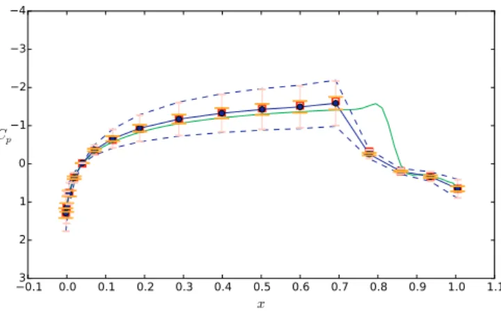
Fig. 3. PRSV model: posterior predictive distributions (p.p.d.) of the pressure coefficient based on various calibration scenarios. Data Cp jref, (¤), nominal Cp jNom, .( )

and posterior E C C[ |p p jref,,PRSV]( ). Error bars (E C C[ |p p jref,,PRSV]±S C C[ |p p jref,,PRSV]): experimental uncertainty e ( ), parametric and model uncertainty ηy

( ), total ( ).

Table 5

Calibration results for PRSV - L2-norm error of the residual error with respect to the reference Cpdata.

Scenario Cp jref, Cp jNom, .2 Cp jref, E C C[ |p p jref,,PRSV]2 Cp jref, E C C[ |p pref,123,PRSV] 2

j (Single-point calibration) (Multi-point calibration)

1 1.273 0.130 0.115

2 1.393 1.023 1.032

σ is a measure of the ability of a model to capture the data: the more the

model fails to fit the experimental points, the larger is σ. In other words, if the posterior distribution of the code output y exhibits a weak probability to observe the data, then σ increases to compensate for this discrepancy. In practice, due to model inaccuracy, the statistical model tends to capture the data by increasing the variability of the posterior predictive distribution of the QoI. This is done either through a large

posterior variability of the physical parameter (in this case,cv ), or

through the model-inadequacy term. This is clearly illustrated byFig. 3,

which reports the posterior predictive distributions (p.p.d.) for the

pressure coefficient Cp. These are compared to the nominal solution and

to the data used for the calibration. The expectancy of the p.p.d. is found to be closer to the data for scenario 1 than for scenarios 2 and 3.

However, because of the small standard deviation of cv, ∞and hence of

Fig. 4. Calibration results for PRSV. Posterior predictions for the saturation curve and the transition line =( 0). Panels (a) to (d): nominal saturation curve ( ), nominal transition line ( ), mean posterior saturation curve (+), mean posterior transition line (×) and posterior transition line error bars (•_{). Panel (e):}

reference data based on the SW model ( ), transition line ( ), = 0.3 ( ) and = 0.5 ( ). Panel (f): posterior average and standard

Cpfor this scenario, the reference is assigned a poor chance of

occur-rence and the model-form error term leads to a large variance of the p.p.d. In this figure, the error bars associated with the parametric un-certainties (not reported) are of the order of line thickness, and almost superposed with the average solution. For all cases, the p.p.d. are in better agreement with the reference than the deterministic prediction based on the nominal parameters.

InTable 5we report the L2norm of residual error with respect to the

data for the p.p.d. of Cp. The norm is extended to the 17 chordwise

locations. The table shows that 1) independently on the data used for the calibration, the average posterior predictions always improve over the nominal solution; 2) except for the p.p.d. for scenario 1, the mul-tiple-point calibration provides higher residual errors than the p.p.d. based on individual calibrations, due to the fact that the multi-point calibration represents a tradeoff among the observed data for the var-ious scenarios.

Figure 4illustrates the impact of the calibrations on the predicted thermodynamic behaviour. Specifically, the figure shows posterior predictions for the saturation curve and the transition line in the

Clapeyron diagram. Reference data obtained from the SW model are also reported for reference. It is worth noticing that, according to the SW the = 0 curve is located below the saturation curve, D5 being not a BZT fluid according to this reference model. However, the funda-mental derivative is rather close to zero for a wide range of conditions

in the saturated vapour region (seeFig. 4(e)). Concerning the calibrated

model, several considerations are in order. First of all, the saturation curve is not affected by the calibration, since its location depends only

on the thermal equation of state and not on caloric properties likecv .

Secondly, the average posterior location of the transition line is above the nominal one in all cases, indicating that the calibrated model pre-dicts, in average, a wider inversion zone than the baseline. As a con-sequence, for scenarios 1–3, the fundamental derivative tends to take throughout the flow lower values with respect to the nominal model. This leads in turn to a reduction in the maximum Mach number and, as a consequence, to predictions that match more closely the reference data than the nominal solution. Lastly, the posterior prediction of the transition line varies significantly according to the scenario used for the calibration, as a consequence of the inadequacy of PRSV in reproducing

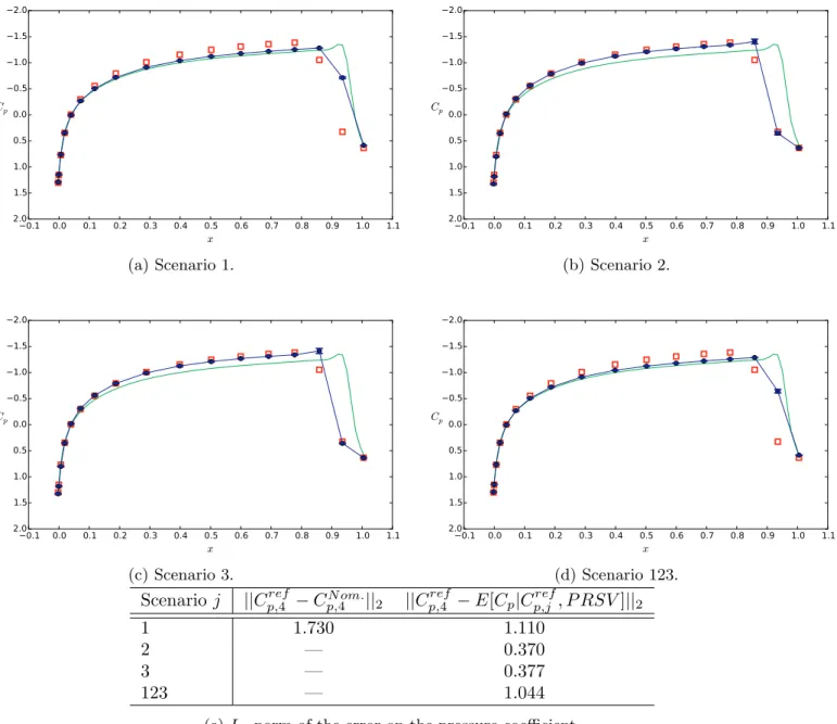
Fig. 5. Prediction results for the calibrated PRSV model. Pressure coefficient for operating point 4: reference data Cpref,4(¤), nominal CpNom,4 .( ) and posterior

Fig. 6. Prediction results for the calibrated PRSV model. Pressure coefficient for operating point 5: reference data Cpref,5(¤), nominal CpNom,5 .( ) and posterior

E C C[ |p p jref,,PRSV]( ). Error bars (E C C[ |p p jref,,PRSV]±S C C[ |p p jref,,PRSV]): parametric uncertainty y ( ).

Fig. 7. PRSV - Drag coefficient predictions. Reference Cdref,{4,5}( ), nominal CdNom,{4,5}.( ), p C C( |d pref,1,PRSV)( ), p C C( |d pref,2,PRSV)( ), p C C( |d pref,3,PRSV)

the fluid thermodynamic behavior correctly in the whole flow field. Interestingly, if the EOS is calibrated directly by using thermodynamic

data (and more specifically pvT data)[50]the inversion zone tends to

disappear (as in the SW model) but predictions of the aerodynamic quantities based on the updated EOS are found to be less accurate than the nominal model. Indeed, in this case the fundamental derivative takes overall higher values throughout the flow, leading to stronger shocks.

Finally, the ability of the calibrated model to predict unobserved flows is investigated by propagating the parameters calibrated against scenarios 1–3 and 123 through scenarios 4 and 5. The results are

de-picted inFigures 5and6, along with validation data obtained by

run-ning the reference SW model and the nominal solutions. The L2-norms

of the errors with respect to the pseudo-experiments are also reported in panel e of both figures. Predictions are based on the sole propagation of the posterior parameter distributions through the new scenario, char-acterized by a small variance. This leads to small uncertainty bounds of the output QoI, which do not always encompass the validation data. This makes us argue that the parametric uncertainty alone is not suf-ficient to capture the “truth”, and that the model-form uncertainty should also be taken into account. Unfortunately, the model-in-adequacy term η can be hardly extrapolated to a scenario different from the calibration ones. In almost all cases, the average predictions are closer to the reference solution than the nominal solution. However, the improvement is more or less important depending on the calibration scenario used to train the parameters. As expected from the posteriors

of cv, ∞, we observe similar distributions for scenarios 2 and 3 on one

side, and for scenarios 1 and 123 on the other side, for both prediction points. The predicted mean distributions based on calibrations against scenarios 2 and 3 show a good adequacy with the reference, with posterior errors of about 0.370-0.377 and 0.143 compared to the nominal errors of 1.730 and 1.719 for the nominal solutions at points 4

and 5, respectively. In particular, the shock location is drastically im-proved and lies very close to the reference. On the other hand, the predicted shock locations based on calibration scenarios 1 and 123 remain very close to the nominal solutions. Note that the prediction scenarios 4 and 5 are rather close to calibration scenarios 2 and 3, which explains the good performance of the model when calibrated against these points. Finally, even if the posterior mean distributions of

Cpare in closer agreement with the reference than the nominal solution,

the error bars do not allow to capture the reference data all along the

airfoils. This is due to the small posterior variance of cv, ∞and to the

lack of a model-form uncertainty term. In other terms, accounting for the parametric uncertainty only leads to a severe underestimation of the solution variance, more notably in the shock region. This point will be discussed further in the following.

To complete the analysis, we finally consider the p.p.d. for a global performance parameter which was not directly informed from the data, i.e. the drag coefficient, given by

=

C D

V

d ₁

2 2

with D= _airfoilpn i·dS the pressure force component in the flow di-rection i. The results are reported inFig. 7for predictions at conditions 4 and 5, based on parameter posteriors calibrated on scenarios 1, 2, 3

and 123, respectively.Table 6 provides the means and the standard

deviations for the various p.p.d.s, along with the value predicted by using the nominal values of the parameters and the pseudo-experi-mental reference.

Due to the linear relationship between Cdand p, the drag coefficient

follows similar trends as the pressure coefficient Cp. However, due to

the sensitivity of this integrated parameter to small variations of the

shock location, Cddistributions are more affected by the parametric

uncertainty. For both prediction scenarios, the average Cdis to within

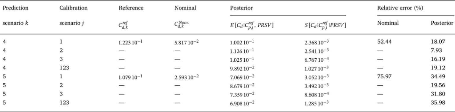
3% and 4% of the reference value, in the best cases (prediction based on scenarios 2 and 3), which represents a considerable improvement over the nominal model results, characterized by relative errors of 21.18% and 26.88%, respectively. The prediction error increases to about 15% when using posteriors calibrated from scenarios 1 and 123. Despite the improvements observed for the prediction of mean values, it appears that the reference values are in general not captured by the posterior distributions of Cdfor any choice of the calibration scenario. In the best

cases, the reference value of Cdis close to the tail of the posterior

dis-tribution.

5.2. Results for the MAH model

In this section we discuss the calibration results for the MAH model. The posterior means and standard deviations of the stochastic

parameters/hyperparameters Tc, σ, α and β are given inTable 7for the

various calibration scenarios (single- and multi-point). Posterior

dis-tributions of the critical temperature Tcare found to be rather similar

Table 6

PRSV - Predictions of the drag coefficient.

Prediction Calibration Reference Nominal Posterior Relative error (%) scenario k scenario j C_{d k}ref

, Cd kNom, . E C C[ |d p jref,,PRSV] S C C[ |d p jref,|PRSV] Nominal Posterior

4 1 1.223 101 _{1.482 10}1 _{1.414 10} 1 _{1.075 10} 4 _{21.18 15.62} 4 2 — — 1.260 10 1 _{1.702 10}3 _{— 3.03} 4 3 — — 1.260 10 1 _{1.055 10} 3 _{— 3.03} 4 123 — — 1.410 10 1 _{2.268 10}4 _{— 15.29} 5 1 1.079 101 _{1.369 10}1 _{1.265 10} 1 _{1.617 10} 4 _{26.88 17.24} 5 2 — — 1.040 10 1 _{2.398 10}3 _{— 3.61} 5 3 — — 1.039 10 1 _{1.471 10}3 _{— 3.71} 5 123 — — 1.258 10 1 _{3.393 10} 4 _{— 16.59} Table 7

MAH model: mean E and standard deviation S of the posterior distributions of the parameters for the various scenarios.

Mean and Std. deviation Scenario j

1 2 3 123 E T C[ |c p jref,,MAH] 573.898 565.746 572.271 574.720 S T C[ |c p jref,,MAH] 1.604 1.485 0.462 0.689 E[ |C_{p j}ref_,,MAH] 0.474 0.247 0.772 0.837 S[ |Cp jref,,MAH] 0.104 0.056 0.773 0.131 E[ |C_{p j}ref_,,MAH] 0.009 0.009 50182.526 0.017 S[ |Cp jref,,MAH] 0.004 0.005 28864.872 0.004 E[ |C_{p j}ref_,,MAH] – – – 0.038 S[ |C_{p j}ref,MAH] , – – – 0.023

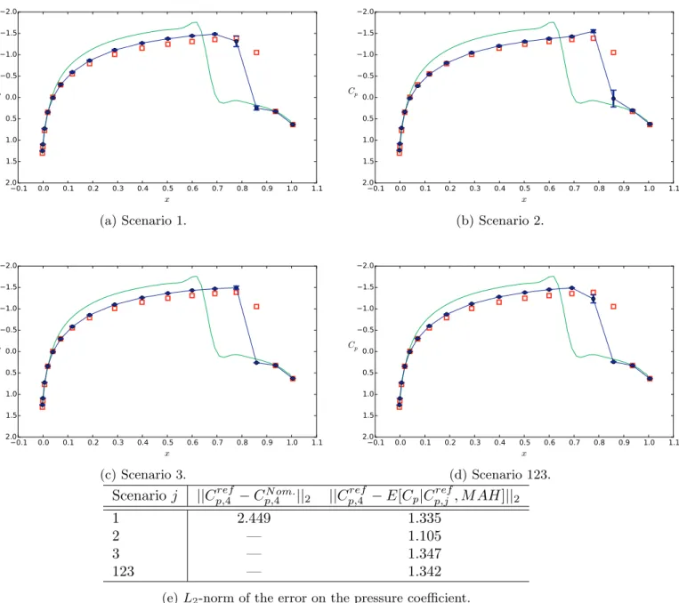
for all calibration scenarios. Indeed, the posterior means range from 565.746 up to 574.720. This are about 8% lower than the nominal value of 619.15. The posterior standard deviations are very small (less than approximately 0.3%) for all cases, showing that this parameter is very well informed from the data, but also that the calibration is very sensitive to the calibration scenario, since the different posteriors do no overlap. Concerning the hyperparameters, the posterior mean of σ ranges from 0.247 (for scenario 2) up to 0.837 (for scenario 123). These

rather high values indicate that the model-form error plays a crucial role for capturing the data, thus compensating the small posterior

variance of the physical parameter Tc.

The posterior distributions of the pressure coefficient for the

cali-bration scenarios, reported inFig. 8, show a good agreement with the

data. For scenarios 1 and 2, the data are located to within one experi-mental standard deviation from the mean posterior prediction, included in the shock region. For point 3, the shock location is predicted less

Fig. 8. MAH model: posterior predictive distributions (p.p.d.) of the pressure coefficient based on various calibration scenarios. Reference Cp jref, (¤), nominal Cp jNom, .

( ) and posterior E C C[ |p p jref,,MAH]( ). Error bars (E C C[ |p p jref,,MAH]±S C C[ |p p jref,,MAH]): experimental e( ), parametric and model uncertainty ηy ( ),

total ( ).

X. Merle, P. Cinnella Reliability Engineering and System Safety 183 (2019) 400–421