Science Arts & Métiers (SAM)
is an open access repository that collects the work of Arts et Métiers Institute of
Technology researchers and makes it freely available over the web where possible.
This is an author-deposited version published in:
https://sam.ensam.eu
Handle ID: .
http://hdl.handle.net/10985/9291
To cite this version :
Antoine DUMAS, Jean-Yves DANTAN, Nicolas GAYTON - Impact of a behavior model
linearization strategy on the tolerance analysis of over-constrained mechanisms -
Computer-Aided Design - Vol. 62, p.152-163 - 2015
Any correspondence concerning this service should be sent to the repository
Administrator :
archiveouverte@ensam.eu
Impact of a behavior model linearization strategy on the tolerance
analysis of over-constrained mechanisms
✩A. Dumas
a,b,∗, J.-Y. Dantan
a, N. Gayton
baLCFC, Arts et Métiers ParisTech Metz, 4 rue Augustin Fresnel, 57078 METZ CEDEX 3, France bClermont Université, IFMA, UMR 6602, Institut Pascal, BP 10448, F-63000 Clermont-Ferrand, France
h i g h l i g h t s
• A tolerance analysis approaches overview is proposed.
• A linearization procedure of the behavior model is required for both approaches. • Some linearization strategies provide conservative probability of failure results. • A confidence interval is obtained using two different linearization strategies. • The order of magnitude of the probability has an effect on the convergence speed.
All manufactured products have geometrical variations which may impact their functional behavior. Tolerance analysis aims at analyzing the influence of these variations on product behavior, the goal being to evaluate the quality level of the product during its design stage. Analysis methods must verify whether specified tolerances enable the assembly and functional requirements. This paper first focuses on a literature overview of tolerance analysis methods which need to deal with a linearized model of the mechanical behavior. Secondly, the paper shows that the linearization impacts the computed quality level and thus may mislead the conclusion about the analysis. Different linearization strategies are considered, it is shown on an over-constrained mechanism in 3D that the strategy must be carefully chosen in order to not over-estimate the quality level. Finally, combining several strategies allows to define a confidence interval containing the true quality level.
1. Introduction
Geometrical tolerances influence both design functional per-formance and production costs, because their effects are felt at all stages of the product life cycle, so these are key elements for the design process. Appropriate design tolerances enable complex mechanical assemblies, made up of several parts, to be assembled and functional at low cost. Moreover, they enable the quality level of assemblies to be increased and ensure a high mechanical reli-ability of the product. To evaluate whether the design tolerances
are relevant to ensure the functionality of the product, a method-ology such as tolerance analysis must be applied. The tolerance analysis of mechanisms aims at verifying whether the specified design tolerances allow to reach a given quality level of the prod-uct during its design stage. The goal is to avoid the manufacturing of non-functional mechanisms. Hence, tolerance analysis is a key element [1]:
•
to improve product quality,•
to reduce manufacturing costs,•
to manage and reduce waste in production.Tolerance analysis can be divided into two approaches, whose techniques to build the behavior model are different. A comparison of both approaches is proposed in order to show their similarities and differences. Although the formulations of the mathematical models are different, both approaches need to deal with an ap-proximated model coming from a linearization procedure in order to perform the analysis method and compute a predicted quality
level. Indeed, the analysis method is based on mathematical op-erations which require a linear model: a Minkowski sum and lin-ear optimization problem with constraints. For both approaches, the linearization procedure implies simplifying the behavior model and thus modifying the accuracy of the mathematical model. This operation creates a model error which needs to be quantified. In addition, depending on the type of linearization, the corresponding error created may be different. It appears interesting to determine the best linearization procedure in order to limit the approxima-tion error.
This paper first proposes a brief comparison of tolerance anal-ysis approaches to show why the linearization procedure is re-quired for both techniques. Then the paper intends to show that the linearization procedure has, of course, a real impact on the predicted quality level and on the computer time to obtain the information. However, a carefully chosen linearization procedure strategy enables this impact to be reduced. Indeed, depending on the considered strategy, the quality level may be under-estimated or over-estimated, and the computing time can be greatly in-creased. The analysis method must therefore take these parame-ters into account when applying a linearization procedure.
The next section of this paper focuses on a literature overview of both tolerance analysis approaches in order to show that a linearization procedure of the behavior model is required for all approaches. Section3presents the considered linearization strate-gies of the behavior model. The mathematical operation for the lin-earization of non-linear equations is detailed. Section4integrates the mathematical description and the solution of a tolerance anal-ysis problem based on the model proposed by Dantan and Qureshi et al. [2,1]. Section5is devoted to an impact analysis of the lin-earization procedure on an industrial application. Results of the linearization impact are shown and discussed in this section. A con-clusion ends the paper.
2. Tolerance analysis overview
Tolerance analysis aims at verifying the value of functional re-quirements after tolerances have been specified on each compo-nent of a mechanism. Three main issues exist [3]:
1. Modeling geometrical deviations due to the manufacturing process and modeling gaps between features.
2. Building a mathematical model to simulate the behavior of the mechanism, taking into account deviations and gaps.
3. Developing analysis methods to estimate the quality level.
2.1. Geometrical models
Modeling geometrical deviations and gaps are required in order to perform items 2 and 3. Both deviation and gap characterize a displacement between two surfaces of a mechanism. The geometry of the mechanism parts can be modeled in different ways:
•
nominal surface: ideal surface whose dimensions and positions match the design.•
skin model: real manufactured surface.•
substitute surface: perfect surface associated with the skin model where the form defects are neglected.In the present paper the form defects are omitted, so the repre-sentation of the geometrical deviations and the gaps is based on substitute surfaces. It could be between two substitute surfaces or between a substitute surface and a nominal surface [2]. Geometri-cal deviations (situation or/and intrinsic deviations) are modeled by random variables, written X
= {
X1, . . . ,
Xn}
. Gaps are modeled by free variables, written G= {
g1,
g2, . . . ,
gm}
, which need to be computed by the analysis method. Small displacements and kine-matic displacements may be considered; they are used either tomodel small mobilities of the mechanism due to deviations and gaps, or kinematic displacements in joints.
Several representations are mentioned in the literature to deal with displacements. They can be expressed using one of the following techniques: kinematic formulation [4,5], small displace-ment torsor (SDT) [6,7], matrix representation [8], vectorial toler-ancing [9]. The analysis method formulation is based on the small displacement torsors, see Section4, but it is not limited to one of these techniques; all representations are suitable.
2.2. Behavior models
Building a behavior model allows to know how features of a mechanism interact, that is why relations characterizing its be-havior have to be identified. In particular, these relations concern dimensional chains, in order to link features in contact with each other, with or without gaps. In addition, other relations have to be considered to prevent features from penetrating into others when there are gaps. Tolerance analysis can be divided into two dis-tinct categories: displacement accumulation and tolerance accu-mulation [1]. The first category defines constraints on parameters [2,1] and the second one defines admissible volumes of variations [10–13].
•
The goal of displacement accumulation is to model the in-fluences of the deviations on the geometrical behavior of the mechanism. The relation uses the following form [14]:Y
=
f(
X,
G)
(1)where Y is the response of the system (a characteristic such as a gap or a functional characteristic). The function f represents the deviation accumulation of the mechanism; it can be an explicit analytical expression, an implicit analytical expression or a nu-merical simulation. The difficulty in determining the function f increases with the complexity of the studied system [15,2,16].
•
The aim of tolerance accumulation is to simulate the com-position of tolerances i.e. linear tolerance accumulation, 3D accumulation. The admissible deviations are mapped using sev-eral vector spaces in a region of hypothetical parametric space. Tolerance accumulation uses relations between all domains to characterize the geometrical behavior. The literature mentions several techniques to represent geometrical tolerances or di-mensioning tolerances, among which are T-maps⃝R [10,17,11],gap spaces [18,19] and deviation domains [12,13].
In both cases, several types of domains and constraints are de-fined. Although the behavior model is based on different math-ematical tools, an analogy between these types is possible. Both representations of mechanical behavior have similarities; a brief parallel of both approaches is presented inTable 1.
2.3. Tolerance analysis problem formulations
The tolerance analysis method must define a mathematical formulation able to take into account all the characteristics of the behavior model and to provide an accurate computed quality level. A comparison of the quality level formulations is presented in Table 2.
Different analysis method techniques exist, such as worst-case analysis and statistical analysis [14,2]:
•
The goal of statistical tolerance analysis is to compute the probability that the requirement can be satisfied under given individual tolerances [14,24,19].•
The worst case analysis method (also called deterministic or high–low analysis method) involves defining the dimensions and tolerances such that any possible combination of work-pieces provides an admissible assembly of the mechanism. In the examination of the functional requirement, the worst pos-sible combination of each deviation is considered [25,26].Table 1
Comparison of the behavior models between the displacement accumulation approach and the tolerance accumulation approach.
Displacement accumulation Tolerance accumulation
•Deviation constraints: •Deviation volume:
Probability distributions Vd(X,G)
Random variables whose distributions and parameter values are known, e.g. X∼N(µX, σX), [1].
Deviation space (T-Maps⃝R[11,20], deviation domains [20]) representing the
admissible variations of a feature within its tolerance zone.
•Interface constraints: •Clearance volume:
Ci(X,G) ≤0 and Ci∗(X,G) =0 Vc(X,G)
Characterize the non-interference or association between substitute surfaces, which are nominally in contact, by limiting gaps between them [1].
Hypervolume of admissible variations (i.e. without interference) of a frame with respect to another [20]. Frequency distributions are also used in
T-Maps⃝R
approach [21].
•Functional condition: •Functional volume:
Cf(X,G) ≤0 Vf(X,G)
Limits the orientation and the location between surfaces in relative displacement, which are in functional relation [1].
Specific volume characterizing the admissible variation space of an assembly so as to satisfy the functional requirement [20].
•Compatibility equations: •Relation between volumes:
Cc(X,G) =0 Vd1(X,G) ⊕Vd2(X,G) ⊖Vc1(X,G)
Geometrical behavior of the mechanism expressed by the composition relations of displacements in various topological loops [1].
Minkowski sums or intersections performed according to the different dimensional chains of the mechanism on hypervolumes to obtain accumulated volumes [20].
Table 2
Comparison of tolerance analysis methods between the displacement accumulation approach and the tolerance accumulation approach.
Displacement accumulation Tolerance accumulation
•Assembly requirement: The assembly of a mechanism with gaps must be ensured. The various features, in the presence of
deviations, must be assembled without interfering with each other.
◦‘‘there exists an admissible gaps configuration of the mechanism such that the assembly requirement (interface constraints) and the compatibility equations are respected’’ [1].
∃G∈Rm:Cc(X,G) =0
Ci(X,G) ≤0
Ci∗(X,G) =0
◦In this case, the assembly requirement is satisfied when the intersection of all accumulated clearance domains is not empty [20].
Vd(X,G) ⊂ Vc(X,G)
•Functional requirement: Once the assembly requirement is verified, the influence of the geometrical deviations can be evaluated on
a functional characteristic, which is basically a maximum or a minimum clearance on a feature which has an impact on the performance of the mechanism.
◦‘‘for all admissible gap configurations of the mechanism, the geometrical behavior and the functional requirement are respected’’ [1]. ∀G∈ G∈Rm:Cc(X,G) =0 Ci(X,G) ≤0 Ci∗(X,G) =0 : Cf(X,G) ≥0
◦The functional requirement is satisfied when the accumulated deviation and clearance domain remains within the functional domain [20].
Vd(X,G) ⊕Vc(X,G) ⊂ Vf(X,G) •Mathematical tools: For both requirements, an optimization
algorithm is required, taking into account all defined constraints. The formulation is detailed in Section4.1. Cylinder joints result in quadratic interface constraints, making the optimization problem more difficult to solve. A solution is to linearize these constraints.
•Mathematical tools: In order to be able to apply Minkowski sums or
intersections to compute accumulated hypervolumes, domains have to be linear. A cylinder type joint in a mechanism leads to the definition of a non-linear clearance domain, so it has to be linearized in several facets [22,23].
2.4. Conclusion
Tolerance analysis approaches are based on different tech-niques to provide the quality level of a designed mechanism. The formulation to check the assembly requirement and the functional requirement are different, and hence the required mathematical tools are also different. However, neither method can deal with a non-linear behavior model, i.e. model with quadratic constraints coming from cylinder joints. For tolerance displacement, the use of an optimization algorithm is required to determine the gap val-ues. Qureshi et al. noticed in [1] that in some cases the result was not admissible, because the given result violates constraints dur-ing the resolution. Usdur-ing numerical simulations, up to 10% of the results were not admissible. It is then not conceivable to perform simulations with such a high loss percentage. A possible solution is to use other types of optimization algorithms, such as genetic or evolutionary algorithms. However, these algorithms are very time-consuming so they cannot be used in numerical simulation such as Monte Carlo simulation. In addition, with a non-linear optimiza-tion algorithm, the global minimum may not be found (required for
the functional condition) whereas the global minimum is found in linear programming. For tolerance accumulation, in order to com-pute the accumulated domains, Minkowski sums or the intersec-tion of domains must be applied. These operaintersec-tions require dealing with linear domains to be applied [11,22,23]. Based on these two reasons, we chose to linearize the non-linear equations of the be-havior model. The present paper focuses on studying the impact of such a simplification of the behavior model on the computed qual-ity level. This is based on the displacement accumulation approach, but the previous analogy has shown that this study is also relevant for the tolerance accumulation approach. Using the displacement accumulation approach, the quality level corresponds to the prob-ability of failure to be evaluated, one relative to the assembly re-quirement and one relative to the functional rere-quirement.
3. Linearization procedure for the behavior model
Some interface constraints or deviation domain are written in a quadratic form and they need to be linearized. For instance, com-puting the distance between two points leads to defining nonlinear
Fig. 1. Admissible area of displacement of the pin center (Op) with respect to
the pin hole center (Ob). The variables u andvcorrespond respectively with the
distance between both points along the x-axis and y-axis and dband dpcorrespond
respectively with the diameter of the pin hole and the pin.
equations. Indeed, the distance between the point A of coordinates
(
xA,
yA)
and the point B of coordinates(
xB,
yB)
is expressed as fol-lows:d
(
A,
B) =
(
xA−
xB)
2+
(
yA−
yB)
2.
(2)In order to remove the square root, it is better to deal with the squared distance which provides a quadratic equation. As an ex-ample, the displacement of a pin center with respect to the pin hole center is limited in order to prevent the pin from penetrating into the body.Fig. 1shows the quadratic interface constraint and de-viation domain characterizing the limit distance between the pin center and the pin hole center. This distance must not exceed the radius difference.
Let the quadratic function, to be linearized, be written as de-fined by Eq.(3). The considered strategies are based on a first-order linearization of function Ci to the point Pk of coordinates
(1
R cosθ
k,
1R sinθ
k)
, where1R is the radius difference andθ
k=
2kπ
Nd , for k
=
1, . . . ,
Nd, is an angle whose parameter Ndenables thenumber of linearizations to be adjusted.
Ci
(
u, v) =
u2+
v
2−
1R2.
(3)Linearization corresponds to a discretization of the admissible area of displacement, which is a 2D circle, into a polygon whose num-ber of facets depends on Nd. Nevertheless, this operation does not correspond to a discretization of the geometry. It is the quadratic constraint that corresponds to a circle equation that is linearized. Several Linearization strategies are considered: seeFig. 2. Given
Ci
(
X,
G) =
u2+
v
2−
1R2≤
0, an interface constraint, the lin-earization operation provides new inequalities depending on the type of linearization:Type 1: linearization following an inner polygon:
Ci(k)
(
X,
G) =
u cosθ
k+
v
sinθ
k−
1R cosθ
1
2
≤
0Type 2: linearization following a medium polygon (average
between inner and outer polygons):
Ci(k)
(
X,
G) =
u cosθ
k+
v
sinθ
k−
1R 2
1+
cosθ
1 2
≤
0Type 3: linearization following an outer polygon:
Ci(k)
(
X,
G) =
u cosθ
k+
v
sinθ
k−
1R≤
0with
θ
1=
2Nπd and∆R>
0. One interface constraint becomes Nd interface constraints, increasing significantly the number of con-straints, but these constraints have the advantage of being linear in displacement.Fig. 2. The 3 types of linearization of the real admissible area of displacement, here
with 6 facets.
Fig. 3. Electrical connector.
Fig. 3shows an industrial electrical connector where such a lin-earization procedure is required. Indeed, the mechanism has two cylinder joints, which will involve writing quadratic constraints.
4. Mathematical formulation and solution method for a tolerance analysis problem
This section presents the formulation of the tolerance analysis problem based on the displacement accumulation approach and the applied solution method to compute the probabilities of failure. This method is first proposed by Qureshi et al. [1].
4.1. Formulation of a tolerance analysis problem
According toTable 1, the behavior model comprises three types of equation: interface constraints, compatibility equations and a functional condition. Assuming X is the vector of the geometrical deviations modeled by random variables and G the vector of the gaps, let the set of interface constraints be:
Ci(j)
(
X,
G) ≤
0
j=1,...,NCi
(4) where NCi is the number of interface constraints. Let the set of
compatibility equations be:
Cc(k)
(
X,
G) =
0
k=1,...,NCc (5)
where NCc is the number of compatibility equations.
It is specified inTable 2that to check the assembly requirement it is only necessary to find at least one configuration (a specific set of gaps) such that the interface constraints and compatibility equations are satisfied.
The defect probability, Pfa, for the assembly requirement is given by the following equation:
Pfa
=
1−
Prob
∃ ˜
G|
Ci(
X, ˜
G) ≤
0
whereG is a vector of gaps verifying the set of compatibility equa-
˜
tions
Cc(k)
(
X, ˜
G) =
0
for k
=
1, . . . ,
NCc. The method tocom-pute this probability is to maximize the sum of gaps with interface constraints; a solution reveals the existence of an admissible con-figuration of gaps such that all constraints and equations are satis-fied, whereas if no solution can be provided, it means that at least one constraint is violated, thus the assembly is not possible be-cause there is at least one interference between two components of the mechanism. The defect probability is given by the equation as follows: Pfa
=
Prob
@ max ˜ G ˜
G with Ci(1)(
X, ˜
G) ≤
0...
Ci(NCi)(
X, ˜
G) ≤
0
(7)where the maximization of the sum of gaps is an artificial function. The goal is only to know if a solution can be found to satisfy all the given constraints.
The functional requirement consists of checking whether a functional characteristic Y respects its assigned threshold Yth. The functional condition Cf
(
X,
G) =
Yth−
Y(
X,
G) ≥
0 is defined and must be verified for all admissible gap configurations, seeTable 2. However, all configurations do not have to be checked, indeed, in order to compute the defect probability, it is necessary to find at least one admissible configuration where the functional condition is not respected: Pf=
Prob
∃ ˜
Gadmissible|
Cf(
X, ˜
G) ≤
0
(8) whereG˜
admissibleare gaps values verifying all interface constraintsand compatibility equations. This corresponds with finding the worst gap configuration; this configuration provides the worst value of the functional condition. The technique to find the worst admissible configuration of gaps for the functional condition is to minimize Cfwith interface constraints:
Pf
=
Prob
min ˜ G Cf(
X, ˜
G) ≤
0 with Ci(1)(
X, ˜
G) ≤
0...
Ci(NCi)(
X, ˜
G) ≤
0
.
(9)4.2. Solution method based on Monte Carlo simulation and optimiza-tion
The classic solution method combines a Monte Carlo simulation and an optimization algorithm [1]. As all constraints and functional conditions are linear, an optimization scheme using a simplex technique is chosen to solve both optimization problems defined in Eqs.(7)and(9). The different steps of the solution procedure are described below:
1. A Monte Carlo population is defined: nMC sampling of the random variables, X(i)
,
i=
1, . . . ,
nMC.
2. The optimization algorithm is launched for each sample (either maximization of the sum of gaps or minimization of the functional condition).
3. The probabilities of failure are estimated using the following equation:
˜
Pfa,f=
1 nMC nMC
i=1 ID(
x(i))
(10)Fig. 4. Gear pump.
where ID
(
X)
is the indicator function; for the assembly require-ment the function is:IDfa
(
X) =
1 if no solution can be provided
0 if a solution is found
.
(11) For the functional requirement it is defined as follows:IDf
(
X) =
1 if Cf
(
X) ≤
00 if Cf
(
X) >
0.
(12)N.B.: Beaucaire et al. [24] propose a new solution method to deal with overconstrained mechanisms based on a decomposition of the mechanism into several main configurations. Considering these configurations, the probability formulation becomes the probability of an intersection of events, each event being associated to one specific configuration. Due to the linearization procedure, the number of events may increase considerably, which is why this new formulation is not used in the initial phase.
5. Impact of the linearization procedure on an industrial application
The application is based on a gear pump, seeFig. 4, which has two parts positioned with two pins.Fig. 5shows a half pump view. The joint between the two positioned parts is a planar contact. The positioning of these two parts has an influence on the angle of both gear axes. The functionality of the pump can be reduced if the assembly precision of the parts is insufficient.
Based on this pump, a simplified over-constrained mechanism is studied.Fig. 6shows the mechanism with amplified gaps be-tween parts. This is a 3D version of the 2D mechanism used to il-lustrate the linearization procedure in Section3. Both pins (3) and (4) are fixed to part (2) so as to have only two parts in relative movement. In addition, the planar contact a between (1) and (2) is assumed to be perfect, thus without gaps; only kinematic dis-placements are possible for this joint. The functional requirement concerns the deviation of point G of part (1) with respect to part (2). This point G can be seen as a functional point representative of one axis of the gear pump.
5.1. Behavior model of the mechanism
The model behavior is briefly described in the following sec-tions. The complete equations are given inAppendix A.
Fig. 5. Half gear pump.
Fig. 6. Mechanism in 3D.
Dimensions between points are deterministic; point A is used as an origin to define the coordinates of the other points. A set of parameters is defined,
{
l1, . . . ,
l11}
, to model these dimensions.Fig. 7shows the joint graph of the mechanism where deviation torsors and clearance torsors are represented. Deviation torsors
Tia/iare defined to model the geometrical deviations of a substitute surface ia with respect to the nominal surface i. A torsor is com-posed of three rotation components a, b and c and three translation components u,
v
andw
. Each torsor depends on the type of surface to model. For example, the deviation torsor of the substitute sur-face 1b with respect to the nominal sursur-face 1 is defined as follows:
T1b/1 =
a 1b1 u1b1 b1b1v
1b1 0 0
A.
(13)The other deviation torsors required are
T2b/2
,
T1a/1
,
T2a/2
,
T1c/1
,
T2c/2
,
T1g/1
and
T2g/2
. They are defined in Ap-pendix A.1. Moreover, intrinsic deviations are considered: the di-ameters of the pins and their pin holes: d1b, d3b, d1c and d4c. All
these parameters are modeled using random variables with a nor-mal distribution.
Gaps between joints are modeled by clearance torsors:
G1a/2a
,
G3b/1b
,
G4c/1c
and
G2g/1g
. According to the assumptions, there are no clearance torsors between pins (3), (4) and their pin holes in part (2):
G3b/2b
=
G4c/2c
= {
0}
. Additionally, the torsor
G1a/2a
only represents the kinematic displacement because the joint is assumed to be without gaps. Their form is shown in Appendix A.1. Gaps are the optimization parameters
when checking the assembly requirement, see Eq.(7), or finding the worst gap configuration, see Eq.(9).
Fig. 8shows the top view of the mechanism with amplified de-viations and gaps. Only translation components of the deviation torsor and clearance torsor can be represented.
Compatibility equations are written using topological loops of the joint graph, seeFig. 7. There are 5 joints and 4 workpieces (without taking into account the functional joint) so 2 assembly requirement topological loops are studied (Njoints
−
Nworkpiece+
1) which provides 12 linear equations. The loops used are written below:•
Loop (1), (2), (3), expressed in A:
T1/1
A= {
0}
=
T1/1b +
G1b/3b +
G3b/2b +
T2b/2
+
T2/2a +
G2a/1a +
T1a/1
.
(14)•
Loop (1), (3), (2), (4), expressed in A:
T1/1
A= {
0}
=
T1/1b +
G1b/3b +
G3b/2b +
T2b/2
+
T2/2c +
G2c/4c +
G4c/1c +
T1c/1
.
(15)Equations obtained with these loops are detailed inAppendix A.2. The functional condition is written using a topological loop go-ing through the functional condition. The loop (1), (3), (2), Cf ex-pressed in G is taken to obtain a relationship with the functional characteristics u2g/1gand
v
2g/1g:
T1/1
G= {
0} =
T1/1b +
G1b/3b +
G3b/2b +
T2b/2
+
T2/2g +
G2g/1g +
T1g/1
.
(16)This loop provides two equations with which the functional char-acteristic can be written; this is the sum of the displacement u2g/1g
and
v
2g/1g:u2g1g
+
v
2g/1g=
u1b1+
l9b1b1+
u3b1b−
l8C3b1b+
l9b3b1b−
u2b2−
l9b2b2+
u2g2−
u1g1+
v
1b1−
l9a1b1+
v
3b1b−
l9a3b1b+
l7C3b1b−
v
2b2+
l9a2b2+
v
2g2−
v
1g1.
(17)This characteristic must not exceed a threshold dth; the functional condition is given as follows:
Cf
(
X,
G) =
dth−
(
u2g1g+
v
2g/1g) ≥
0.
(18)The non-interference conditions must be checked for two joints: surface b between pin (3) and pin hole (1) and surface c be-tween pin (4) and pin hole (1).
•
Non-interference 1b/
3b: Ci(1)=
u23b1b+
v
3b1b2−
d1b−
d3b 2
2≤
0 (19) Ci(2)=
(
u3b1b+
l3b3b1b)
2+
(v
3b1b−
l3a3b1b)
2−
d1b−
d3b 2
2≤
0.
(20)•
Non-interference 1c/
4c: Ci(3)=
u24c1c+
v
24c1c−
d1c−
d4c 2
2≤
0 (21) Ci(4)=
(
u4c1c+
l4b4c1c)
2+
(v
4c1c−
l4a4c1c)
2−
d1c−
d4c 2
2≤
0.
(22)Fig. 7. Joint and deviation graph associated with the studied mechanism in 3D.
Fig. 8. Top view of the mechanism with amplified deviations and gaps. Intrinsic
deviations are represented for pins (3): d1b and d3b. In addition, deviations of surfaces 1c and 2c with respect to their nominal surface are represented:
u1c1, v1c1,u2c2, v2c2. Point Cnominalcorresponds to the case where no deviations are
considered. Gaps components for joint 1c/4c are also shown: u4c1candv4c1c.
These four inequalities are linearized following the different strate-gies proposed in Section3.
5.2. Numerical results
All parameter values: dimensions, means, standard deviations and probability laws, are necessary for tolerance analysis. Pins diameters and situation deviations are defined as random variables following a normal distribution. Several standard deviation values are set in order to obtain different orders of magnitude of probabilities of failure. Monte Carlo simulations are performed on three different populations. The number of samples nMCis chosen in order to yield a coefficient of variation on the probability of failure (see Eq.(23)) of lower than 5%.
C.O.V.Pf
=
1
−
PfPfnMC
.
(23)Fig. 9shows the variation in computing time for each simulation as a function of the number of linearizations. The required time
Fig. 9. Evolution of computing time as a function of the number of linearizations
and for different orders of magnitude for the probability of failure. Simulation performed with an Intel Core i7-2720.
is naturally longer for a larger number of linearizations because the constraint optimization problem is more complex to solve. Secondly, the order of magnitude of the probability has a strong influence on the computing time; indeed the dash–dot curve with triangle markers represents the smallest target probability and the computing time increases faster than for the others. Therefore, it is very important to select the best linearization strategy in order to obtain an accurate enough result and to avoid useless computing time.
5.2.1. Impact of the number of linearizations on probability of failure convergence
Only results pertaining to probabilities of around 10−2are
pre-sented in this section. Other results are shown in theAppendices. Numerical results are given inTable 3; the corresponding curves are shown inFigs. 10and11. The results show that the number of
Table 3
Probabilities of failure obtained with the first set of values, order of magnitude 10−2. Set of values 1
Pfa(×10−2) Pf(×10−2)
Nsamples 3e5 3e5
C.O.V. ∼0.7% ∼1.2%
95% C.I. ∼0.18 ∼0.1
Nd Inner Medium Outer Inner Medium Outer
8 6.72 6.37 6.06 1.15 1.61 2.20 12 6.53 6.37 6.23 1.75 2.01 2.31 16 6.48 6.39 6.31 1.81 1.95 2.11 20 6.42 6.37 6.31 1.90 2.01 2.1 25 6.39 6.35 6.32 1.96 2.01 2.09 30 6.38 6.36 6.34 1.97 2.03 2.08 40 6.37 6.36 6.34 1.98 2.01 2.03 50 6.37 6.36 6.35 2.01 2.02 2.04 60 6.36 6.36 6.35 2.01 2.02 2.03 70 6.36 6.36 6.36 2.02 2.02 2.03
Fig. 10. Convergence of the probability of failure of the assembly requirement for
the first set of values.
linearizations Ndand the strategy influence the probability of fail-ure values. Strategies provide different results which all converge toward the same value, validating the linearization equations. De-pending on the requirement, one specific strategy is more inter-esting than another. Considering a target probability to be reached, the inner polygon strategy provides conservative results for the as-sembly requirement. In this case, even if the result is an approxi-mation, the probability will not be underestimated. This strategy may be preferred when only one result is expected. On the con-trary, for the functional requirement, the conservative results are provided by the outer polygon strategy. Furthermore, the combi-nation of the inner and outer polygon strategies provides a con-fidence interval for the true failure probability value. The greater the number of linearizations, the smaller the confidence interval. The medium polygon strategy gives the best results, which are very close to the converged value; however these values may not be conservative, which may not be suitable. Yet this strategy may be preferred if a simple approximation of the order of magnitude is required.
5.2.2. Impact of the probability order of magnitude on convergence speed
The previous results concern the impact of the number of lin-earizations, but the order of magnitude of the target probability can also have an impact. Indeed, the order of magnitude may have an influence on the required number of linearizations to reach a
Fig. 11. Convergence of the probability of failure of the functional requirement for
the first set of values.
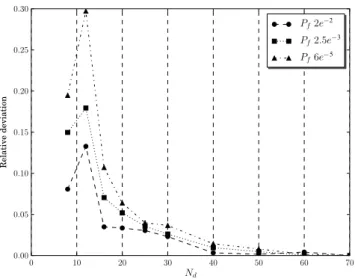
Fig. 12. Relative deviation of Pfafor the inner strategy.
certain accuracy.Figs. 12and13show the relative deviation be-tween the approximate probability and its converged value for the conservative strategy of the assembly and functional requirement. These figures show that the smaller the real probability, the greater the relative deviation. It means that for a given number of lineariza-tions, the relative deviation between the approximated probability and the real probability is greater for a small probability (e.g. 10−6)
than for a greater probability (e.g. 10−2). This means that a smaller real probability requires a finer linearization to reach the same ac-curacy than a greater real probability. In a same way, for a given number of linearizations, the confidence interval of the probability of failure is larger when the real probability is small.
6. Conclusion
The functionality of a product is influenced by design toler-ances. Evaluating the quality level of a product at its design stage is therefore a key element, enabling an improvement of the func-tional quality of the product while reducing the manufacturing cost. This requires methods such as tolerance analysis to quan-tify the impact of tolerances on mechanism quality. To evaluate the quality level of the product, a mathematical model is required, which must represent its behavior as well as possible. However, the behavior model may be approximated. Therefore the objective
Fig. 13. Relative deviation of Pffor the outer strategy.
of this paper is to answer two questions: ‘‘Why is an approxima-tion required?’’ and ‘‘What is its impact on the predicted quality level?’’.
The paper proposed by Qureshi et al. [1] provides a tolerance analysis formulation able to deal with non-linear behaviors. Al-though the mathematical formulation enables this kind of prob-lem to be solved, a difficulty appears when calling the optimization scheme with non-linear constraints. Some optimization operations do not converge, making the result unreliable. The present paper is dedicated to defining linearization strategies for the non-linear constraints in order to solve this difficulty. The goal is to demon-strate that applying a linearization procedure has an impact on the predicted quality level (probability of failure). The outcomes of the study are listed below:
•
The linearization of non-linear equations is required in both tol-erance analysis approaches: toltol-erance accumulation and dis-placement accumulation.•
The linearization of non-linear constraints has a real impact on the probability of failure of the mechanism; the obtained result may underestimate the real value, hence over-estimating the quality of the design. The linearization procedure must be cho-sen carefully in order to obtain conservative results. Indeed, de-pending on the type of requirement, the conservative strategy is different: inner polygon strategy for the assembly requirement and outer polygon strategy for the functional requirement.•
An interesting procedure consists of defining a confidence in-terval of the true probability of failure using two lineariza-tion strategies: outer and inner polygon. This interval becomes smaller when the number of linearizations increases.•
Approximation due to linearization is all the more important when the real probability of failure is small. This means that the number of linearizations must be greater for a small probability in order to obtain the same accuracy for the results.Future studies will concern the establishment of a smart algorithm, able to re-use results obtained from a simulation with a poor pre-cision. The idea is that between a simulation with poor precision and one with good precision, a large number of points in the Monte Carlo simulation give the same result. Using the results with poor precision, the goal is to evaluate only those points which may have a different result with a greater degree of linearization. Hence, the computing time to yield an accurate result can be considerably re-duced. This algorithm will then be tested on a more complex in-dustrial application.
Acknowledgment
The authors would like to acknowledge the support of ANR ‘‘AHTOLA’’ project (ANR-11- MONU-013).
Appendix A. Behavior model
A.1. Geometrical model
Point A is used as an origin to define the coordinates of the other points:
−
→
AC=
l 1 l2 0
−
→
AB=
0 0 l3
−
→
CD=
0 0 l4
−
→
AE=
0 0−
l5
−
→
CF=
0 0−
l6
−
→
AG=
l 7 l8 l9
−
→
AH=
l 10 l11 0
.
Deviation torsors Tia/iare defined to model the geometrical de-viations of a substitute surface ia with respect to the nominal sur-face i.
T1b/1 =
a 1b1 u1b1 b1b1v
1b1 0 0
A
T2b/2 =
a 2b2 u2b2 b2b2v
2b2 0 0
A
T1a/1 =
a 1a1 0 b1a1 0 0w
1a1
A
T2a/2 =
a 2a2 0 b2a2 0 0w
2a2
A
T1c/1 =
a 1c1 u1c1 b1c1v
1c1 0 0
C
T2c/2 =
a 2c2 u2c2 b2c2v
2c2 0 0
C
T1g/1 =
a 1g1 u1g1 b1g1v
1g1 c1g1w
1g1
G
T2g/2 =
a 2g2 u2g2 b2g2v
2g2 c2g2w
2g2
G.
Other deviations: diameters of the pins and their pin holes: d1b, d3b, d1cand d4c.
Gaps between joints are modeled using clearance torsors:
G1a/2a =
0 U 1a2a 0 V1a2a C1a2a 0
A
G3b/1b =
a 3b/1b u3b/1b b3b/1bv
3b/1b C3b/1b W3b/1b
A
G4c/1c =
a 4c/1c u4c/1c b4c/1cv
4c/1c C4c/1c W4c/1c
C
G2g/1g =
−
u 2g/1g−
v
2g/1g−
−
G.
A.2. Compatibility equations
Loop (1), (2), (3), expressed in A, gives the following compati-bility equations:
Cc(1)
(
X,
G) = −
a1b1−
a3b1b+
a2b2−
a2a2+
a1a1=
0 (A.1) Cc(2)(
X,
G) = −
b1b1−
b3b1b+
b2b2−
b2a2+
b1a1=
0 (A.2)Cc(3)
(
X,
G) = −
C3b1b−
C1a2a=
0 (A.3)Cc(4)
(
X,
G) = −
u1b1−
u3b1b+
u2b2−
U1a2a=
0 (A.4) Cc(5)(
X,
G) = −v
1b1−
v
3b1b+
v
2b2−
V1a2a=
0 (A.5) Cc(6)(
X,
G) = −
W3b1b−
w
2a2+
w
1a1=
0.
(A.6)Loop (1), (3), (2), (4), expressed in A, gives the following compati-bility equations: Cc(7)
(
X,
G) = −
a1b1−
a3b1b+
a2b2−
a2c2+
a4c1c+
a1c1=
0 (A.7) Cc(8)(
X,
G) = −
b1b1−
b3b1b+
b2b2−
b2c2+
b4c1c+
b1c1=
0 (A.8) Cc(9)(
X,
G) = −
C3b1b+
C4c1c=
0 (A.9) Cc(10)(
X,
G) = −
u1b1−
u3b1b+
u2b2−
u2c2+
u4c1c+
l2C4c1c+
u1c1=
0 (A.10) Cc(11)(
X,
G) = −v
1b1−
v
3b1b+
v
2b2−
v
2c2+
v
4c1c−
l1C4c1c+
v
1c1=
0 (A.11) Cc(12)(
X,
G) = −
W3b1b−
l1b2c2+
l2a2c2+
W4c1c+
l1b4c1c−
l2a4c1c+
l1b1c1−
l2a1c1=
0.
(A.12)A.3. Functional condition
The functional characteristic is given by:
u2g1g
+
v
2g/1g=
u1b1+
l9b1b1+
u3b1b−
l8C3b1b+
l9b3b1b−
u2b2−
l9b2b2+
u2g2−
u1g1+
v
1b1−
l9a1b1+
v
3b1b−
l9a3b1b+
l7C3b1b−
v
2b2+
l9a2b2+
v
2g2−
v
1g1.
(A.13)This characteristic must not exceed a threshold dth. The functional condition is given as follows:
Cf
(
X,
G) =
dth−
(
u2g1g+
v
2g/1g) ≥
0.
(A.14) A.4. Interface constraintsThe non-interference conditions concern both pins. Non-interference 1b
/
3b: Ci(1)=
u23b1b+
v
23b1b−
d1b−
d3b 2
2≤
0 (A.15) Ci(2)=
(
u3b1b+
l3b3b1b)
2+
(v
3b1b−
l3a3b1b)
2−
d1b−
d3b 2
2≤
0.
(A.16) Non-interference 1c/
4c: Ci(3)=
u24c1c+
v
4c1c2−
d1c−
d4c 2
2≤
0 (A.17) Ci(4)=
(
u4c1c+
l4b4c1c)
2+
(v
4c1c−
l4a4c1c)
2−
d1c−
d4c 2
2≤
0.
(A.18)A.5. Deviation rotation relations
Rotation deviation expressions for deviation torsors are given as follows:
•
Torsor{
T1a/1}
: a1a1=
l1 l1l11−
l2l10w
1a1,H+
l10−
l1 l1l11−
l2l10w
1a1−
l10 l1l11−
l2l10w
1a1,C (A.19) b1a1=
l2 l1l11−
l2l10w
1a1,H+
l11−
l2 l1l11−
l2l10w
1a1−
l11 l1l11−
l2l10w
1a1,C.
(A.20)•
Torsor{
T2a/2}
: a2a2=
l1 l1l11−
l2l10w
2a2,H+
l10−
l1 l1l11−
l2l10w
2a2−
l10 l1l11−
l2l10w
2a2,C (A.21) b2a2=
l2 l1l11−
l2l10w
2a2,H+
l11−
l2 l1l11−
l2l10w
2a2−
l11 l1l11−
l2l10w
2a2,C.
(A.22)•
Torsor{
T1b/1}
: a1b1=
v
1b1−
v
1b1,B l3 (A.23) b1b1=
u1b1,B−
u1b1 l3.
(A.24)•
Torsor{
T2b/2}
: a2b2=
−
v
2b2+
v
2b2,E l5 (A.25) b2b2=
−
u2b2,E+
u2b2 l5.
(A.26)•
Torsor{
T1c/1}
: a1c1=
v
1c1−
v
1c1,D l4 (A.27) b1c1=
u1c1,D−
u1c1 l4.
(A.28)•
Torsor{
T2c/2}
: a2c2=
−
v
2c2+
v
2c2,F l6 (A.29) b2c2=
−
u2c2,F+
u2c2 l6.
(A.30)Appendix B. Parameter values
Nominal values for the three set of values:
l1 l2 l3 l4 l5 l6 l7 l8 l9 l10 l11 100 40 30 30 20 20 120 50 40 50
−
30 Threshold values: yth Set of values 1 2 3 0.25 0.25 0.28 Random variables:µ
Xσ
XSet of values All 1 2 3
d1b 20 0.06 0.01 0.01 d3b 19.8 0.06 0.01 0.01 d1c 20 0.06 0.01 0.01 d4c 19.8 0.06 0.01 0.01 t 0 0.01 0.01 0.009 r 0 0.01 0.01 0.0009
where t is the vector of the translation components of the geometrical deviations:
t
= {
u1b1, v
1b1,
u1b1,B, v
1b1,B,
u2b2, v
2b2,
u2b2,E, v
2b2,E, w
1a1,
w
1a1,H, w
1a1,C, w
2a2, w
2a2,H, w
2a2,C,
u1c1, v
1c1,
u1c1,D,
v
1c1,D,
u2c2, v
2c2,
u2c2,F, v
2c2,F,
Table C.4
Probabilities of failure obtained with the second set of values. Set of values 2
Pfa(×10−4) Pf(×10−3)
Nsamples 3e6 3e6
C.O.V. ∼4.8% ∼1.15%
95% C.I. ∼0.27 ∼0.12
Nd Inner Medium Outer Inner Medium Outer
8 1.44 0.71 0.42 1.28 1.93 2.9 12 1.62 1.22 0.91 2.07 2.49 2.98 16 1.88 1.62 1.36 2.21 2.45 2.7 20 1.55 1.37 1.26 2.33 2.48 2.66 25 1.52 1.43 1.36 2.41 2.5 2.62 30 1.5 1.42 1.35 2.45 2.52 2.59 40 1.43 1.38 1.36 2.47 2.51 2.55 50 1.48 1.45 1.42 2.49 2.52 2.54 60 1.43 1.42 1.4 2.49 2.51 2.53 70 1.44 1.42 1.42 2.5 2.52 2.52
Fig. C.14. Convergence of the probability of failure of the assembly requirement
for the second set of values.
Fig. C.15. Convergence of the probability of failure of the functional requirement
for the second set of values.
and r is the vector of the rotation components of the geometrical deviations:
r
= {
a1g1,
b1g1,
c1g1,
a2g2,
b2g2,
c2g2}
.
Appendix C. Results for the second set of values
SeeTable C.4,Figs. C.14andC.15.
Table D.5
Probabilities of failure obtained with the third set of values. Set of values 3
Pfa(×10−5) Pf(×10−5)
Nsamples 1e7 1e7
C.O.V. ∼6% ∼4%
95% C.I. ∼0.6 ∼0.1
Nd Inner Medium Outer Inner Medium Outer
8 2.28 1.07 0.47 2.26 4.10 7.48 12 2.63 1.98 1.32 4.65 6.16 8.12 16 3.18 2.63 2.20 4.98 5.87 6.93 20 2.50 2.25 2.05 5.44 6.09 6.66 25 2.42 2.35 2.16 5.81 6.18 6.51 30 2.39 2.24 2.19 5.98 6.23 6.49 40 2.27 2.24 2.19 6.04 6.18 6.35 50 2.39 2.33 2.27 6.13 6.21 6.31 60 2.27 2.24 2.24 6.12 6.19 6.27 70 2.32 2.27 2.24 6.17 6.20 6.26
Fig. D.16. Convergence of the probability of failure of the assembly requirement
for the third set of values.
Fig. D.17. Convergence of the probability of failure of the functional requirement
for the third set of values.
Appendix D. Results for the third set of values
SeeTable D.5,Figs. D.16andD.17.
References
[1] Qureshi A, Dantan J, Sabri V, Beaucaire P, Gayton N. A statistical tolerance analysis approach for over-constrained mechanism based on optimization
and monte carlo simulation. Comput Aided Des 2012;44:132–42
http://dx.doi.org/10.1016/j.cad.2011.10.004.
[2] Dantan J, Qureshi A. Worse case and statistical tolerance analysis based on quantified constraint satisfaction problems and monte carlo simulation. Com-put Aided Des 2009;41(1):1–12.http://dx.doi.org/10.1016/j.cad.2008.11.003. [3] Dantan J, Gayton N, Dumas A, Etienne A, Qureshi A. Mathematical issues
in mechanical tolerance analysis, presented at: 13th Colloque National AIP Priméca, Le Mont–Dore. 2012, pp. 12p.
[4] Desrochers A. Geometrical variations management in a multidisciplinary environment with the Jacobian–Torsor model. In: Davidson JK, editor. Models for computer aided tolerancing in design and manufacturing. 2007. p. 75–84.
http://dx.doi.org/10.1007/1-4020-5438-6_9.
[5] Loose J, Zhou S, Ceglarek D. Kinematic analysis of dimensional variation propagation for multistage machining processes with general fixture layouts. IEEE Trans Autom Sci Eng 2007;4:141–52
http://dx.doi.org/10.1109/TASE.2006.877393.
[6]Bourdet P, Clément A. Controlling a complex surface with a 3 axis measuring machine. Annal CIRP 1976;25:359–64.
[7] Legoff O, Tichadou S, Hascoet J. Manufacturing errors modelling: two three-dimensional approaches. Proc Inst Mech Eng B 2004;218:1869–73
http://dx.doi.org/10.1177/095440540421801219.
[8]Chase K, Magleby S, Glancy C. Tolerance analysis of 2-D and 3-D mechanical assemblies with small kinematic adjustments. In: Zhang HC, editor. Advanced tolerancing techniques, vol. 218. Wiley; 2004. p. 1869–73.
[9] Gao J, Chase K, Magleby S. Generalized 3-d tolerance analysis of mechanical assemblies with small kinematic adjustments. IIE Trans 1998;30:367–77.
http://dx.doi.org/10.1023/A:1007451225222.
[10] Bhide S, Ameta G, Davidson J, Shah J. Tolerance-maps applied to the straight-ness and orientation of an axis, In: CD ROM Proc., 9th CIRP international sem-inar on computer-aided tolerancing, Arizona State University,
http://dx.doi.org/10.1007/1-4020-5438-6_6.
[11] Davidson J, Shah J. Modeling of geometric variations for line-profiles. J Comput Inf Sci Eng 2012;12:1–10.http://dx.doi.org/10.1115/1.4007404.
[12] Giordan M, Duret D. Clearance space and deviation space: application to three-dimensional chain of dimensions and positions. In: 3rd CIRP design seminar on computer-aided tolerancing.
[13] Giordano M, Samper S, Petit J. Tolerance analysis and synthesis by means of deviation domains, axi-symmetric cases. In: 9th CIRP international seminar on computer-aided tolerancing, Arizona State University,
http://dx.doi.org/10.1007/1-4020-5438-6_10.
[14] Nigam S, Turner J. Review of statistical approaches of tolerance analysis. Comput Aided Des 1995;27:6–15
http://dx.doi.org/10.1016/0010-4485(95)90748-5.
[15] Ballu A, Plantec J-Y, Mathieu L. Geometrical reliability of overconstrained mechanisms with gaps. CIRP Ann Manuf Technol 2009;57:159–62
http://dx.doi.org/10.1016/j.cirp.2008.03.038.
[16] Mhenni F, Serré P, Mlika A, Romdhane L, Rivière A. Dependency between dimensional deviations in overconstrained mechanisms. Conception et Production intégrées (Rabat, Maroc, October 2007) p. 22–4.
[17] Davidson J, Mujezinovic A, Shah J. A new mathematical model for geometric tolerances as applied to round faces. J Mech Des 2002;124:609–22
http://dx.doi.org/10.1115/1.1497362.
[18] Zou Z, Morse E. Applications of the gapspace model for multidimen-sional mechanical assemblies. J Comput Inf Sci Eng 2003;12:22–30.
http://dx.doi.org/10.1115/1.1565072.
[19] Morse E. Statistical analysis of assemblies having dependent fitting conditions, In: ASME (Ed.), International mechanical engineering congress and exposition. 2004, p. 1–5.http://dx.doi.org/10.1115/IMECE2004-61664.
[20] Ameta G, Samper S, Giordano M. Comparison of spatial math models for tolerance analysis: tolerance-maps, deviation domain, and TTRS. J Comput Inf Sci Eng 2012;12:1–10.http://dx.doi.org/10.1115/1.3593413.
[21] Ameta G, Davidson J, Shah J. Effects of size, orientation, and form tolerances on the frequency distributions of clearance between two planar faces. J Comput Inf Sci Eng 2011;11:1–10.http://dx.doi.org/10.1115/1.3503881.
[22] Samper S, Adragna P-A, Favreliere H, Pairel E, Hernandez P. Rigid and elastic precision domains of ball bearings. J Comput Inf Sci Eng 2012;12:1–13.
http://dx.doi.org/10.1115/1.3615686.
[23] Mansuy M, Giordano M, Hernandez P. A generic method for the worst case and statistical tridimensional tolerancing analysis, In: Elsevier (Ed.), Procedia Engineering, 2012, pp. 10p, presented at: 12th CIRP International seminar on computer–aided tolerancing,http://dx.doi.org/10.1016/j.procir.2013.08.042. [24] Beaucaire P, Gayton N, Duc E, Dantan J-Y. Statistical tolerance analysis of over-constrained mechanisms with gaps using system reliability methods. Comput-Aided Des 2013;45:1547–55.http://dx.doi.org/10.1016/j.cad.2011.10.004. [25] Hong Y, Chang T. A comprehensive review of tolerancing research. Int J Prod
Res 2002;40:2425–59.http://dx.doi.org/10.1080/00207540210128242. [26] Mansuy M, Giordano M, Hernandez P. A new calculation method for the worst
case tolerance analysis and synthesis in stack-type assemblies. Comput-Aided Des 2011;43:1118–25.http://dx.doi.org/10.1016/j.cad.2011.04.010.