HAL Id: hal-01111588
https://hal.inria.fr/hal-01111588
Submitted on 12 Feb 2015
HAL is a multi-disciplinary open access
archive for the deposit and dissemination of
sci-entific research documents, whether they are
pub-lished or not. The documents may come from
teaching and research institutions in France or
abroad, or from public or private research centers.
L’archive ouverte pluridisciplinaire HAL, est
destinée au dépôt et à la diffusion de documents
scientifiques de niveau recherche, publiés ou non,
émanant des établissements d’enseignement et de
recherche français ou étrangers, des laboratoires
publics ou privés.
Certified Abstract Interpretation with Pretty-Big-Step
Semantics
Martin Bodin, Thomas Jensen, Alan Schmitt
To cite this version:
Martin Bodin, Thomas Jensen, Alan Schmitt.
Certified Abstract Interpretation with
Pretty-Big-Step Semantics.
Certified Programs and Proofs (CPP 2015), Jan 2015, Mumbai, India.
�10.1145/2676724.2693174�. �hal-01111588�
Certified Abstract Interpretation
with Pretty-Big-Step Semantics
Martin Bodin
Thomas Jensen
Alan Schmitt
Inria Rennes, France [email protected]
Abstract
This paper describes an investigation into developing certified ab-stract interpreters from big-step semantics using the Coq proof as-sistant. We base our approach on Schmidt’s abstract interpretation principles for natural semantics, and use a pretty-big-step (PBS) se-mantics, a semantic format proposed by Charguéraud. We propose a systematic representation of the PBS format and implement it in Coq. We then show how the semantic rules can be abstracted in a methodical fashion, independently of the chosen abstract domain, to produce a set of abstract inference rules that specify an abstract interpreter. We prove the correctness of the abstract interpreter in Coq once and for all, under the assumption that abstract operations faithfully respect the concrete ones. We finally show how to define correct-by-construction analyses: their correction amounts to prov-ing they belong to the abstract semantics.
Categories and Subject Descriptors F.3.1 [Specifying and
Veri-fying and Reasoning about Programs]: Mechanical verification
Keywords Abstract Interpretation; Big-step semantics; Coq
1.
Introduction
Static program analyzers are complex pieces of software that are hard to build correctly. Abstract interpretation [9] is a theory for relating semantics of programming languages which has proven ex-tremely powerful for proving the correctness of static program anal-yses. Programming the theory of abstract interpretation in a proof assistants such as Coq has led to certified abstract interpretation, where static analyzers are developed alongside their correctness proof. This significantly increases the confidence in the analyzers so produced.
In this paper, we study the use of big-step operational semantics as a basis for certified abstract interpretation. Big-step semantics is a semantic framework that can accommodate fine-grained oper-ational features while at the same time keeping some of the com-positionality of denotational semantics. Furthermore, it has been shown to be able to handle large-scale definitions of program-ming languages, as witnessed by the recent JSCert semantics of
Permission to make digital or hard copies of all or part of this work for personal or classroom use is granted without fee provided that copies are not made or distributed for profit or commercial advantage and that copies bear this notice and the full citation on the first page. Copyrights for components of this work owned by others than ACM must be honored. Abstracting with credit is permitted. To copy otherwise, or republish, to post on servers or to redistribute to lists, requires prior specific permission and/or a fee. Request permissions from [email protected].
CPP '15, January 13--14, 2015, Mumbai, India. Copyright © 2015 ACM 978-1-4503-3300-9/15/01…$15.00. http://dx.doi.org/10.1145/2676724.2693174
JavaScript [3]. The latter development is the direct motivation for the work reported here. We present a general Coq framework [4] to build abstract semantics correct by construction out of minimum proof effort.
As JSCert is written in a pretty-big-step (PBS) semantics [7], we naturally decided to use it as foundation for this work. PBS semantics are convenient because they reduce duplication in the definition of the language and because they have a constrained format. These constraints allowed us to define our framework in the most general way, without committing to a particular language—see Sections 2 and 3.
1.1 Abstract Interpretation of Natural Semantics
The principles behind abstract interpretation of natural (big-step) semantics were studied by Schmidt [20]. They form the starting point for the mechanization proposed here, although the final result deviates in several ways from Schmidt’s proposal (see Section 7).
Intuitively, abstract interpretation of big-step semantics consists of the following steps:
•define abstract executions as derivations over abstract domains of program properties;
•show abstract executions are correct by relating them to concrete executions;
•program an analyzer that builds an abstract execution among those possible. Such an analyzer is correct by construction, but its precision depends on the abstract execution returned. The first step in Schmidt’s formal development is a precise def-inition of the notion of semantic tree. These are the derivation trees obtained from applying the inference rules of a big-step semantics to a term. This results in concrete judgments of the form t, E⇓ r.
The abstract interpretation of this big-step semantics starts with a Galois connection (in the form of a correctness relation rel) between concrete and abstract domains of base values (see Section 5.1 for an example). This relation extends in the standard way to compos-ite data structures, to environments, and to judgments of the form
t, E⇓ r. An abstract semantic tree is then taken to be a semantic
tree where the values at the nodes are drawn from the abstract do-main. A central step in the development is the extension of the cor-rectness relation to derivation trees. Written relU, this relation states
that a (concrete) derivation tree is related to an abstract derivation tree if the conclusions are related by rel, and that for every con-crete sub-derivation there exists an abstract sub-derivation that is
relU-related to it. This leads to a way of proving correctness of an abstract interpretation, by checking that each rule from the concrete semantics has a corresponding rule in the abstract semantics.
Our approach is similar: concrete and abstract executions are assemblages of rules. The rules and the syntax of terms are shared
between the concrete and abstract versions. The difference between the two versions is twofold: on the semantic domains (contexts in which the execution occurs, such as state, and results), and the way the rules are assembled. An important feature of our approach is that the soundness of the approach depends neither on the specific abstract domains chosen, nor on the semantics itself, as long as the domains correctly abstract operations on the concrete domain.
Abstract derivation trees may be infinite. Convergence of an analysis is obtained by identifying an invariant in the derivation tree. Whichever invariant the analysis uses, it is correct if the returned derivation belongs to the set of abstract derivations.
To summarize the parametricity of our approach, we describe the steps required to produce a certified analysis. First, our frame-work is parametric in the language used, which thus must be de-fined as a PBS semantics based on transfer functions (see Sections 2 and 3). Next, the framework is also parametric in the abstract do-mains, which must also be defined, along with the abstract transfer functions. Once these functions are shown to correctly abstract the concrete transfer functions, a correct-by-construction abstract se-mantics is automatically defined. Finally, an analysis must be devel-oped. The fact that the result of the analysis belongs to the abstract semantics is a witness that it is correct.
1.2 Organization of the Paper
The paper is organized as follows. We first review the principles behind PBS operational semantics and show its instantiation on a simple imperative language in Section 2. In Section 3 we make a detailed analysis of PBS rules and propose a dependently-typed for-malization of their format. The representation of this forfor-malization in Coq is described in Section 4. Section 5 describes the represen-tation of abstract domains and explains how PBS rules can be ab-stracted in a systematic fashion which facilitates the proof of cor-rectness. Section 6 demonstrates the use of the abstract interpreta-tion for building addiinterpreta-tional reasoning principles and program veri-fiers. Section 7 discusses related work and Section 8 concludes and outlines avenues for further work based on our certified abstract in-terpretation.
2.
Pretty-big-step Semantics
Pretty-big-step semantics (PBS) is a flavor of big-step, or natural, operational semantics which directly relates terms to their results. PBS semantics was proposed by Charguéraud [7] with the purpose of avoiding the duplication associated with big-step semantics when features such as exceptions and divergence are added. In this section, we introduce PBS semantics through a simple While language with an abort mechanism. To simplify the presentation, we restrict the set of values to the integers, and let the value 0 be considered as “false” in the branching statements if and while.
We give some intuition of how a pretty-big-step semantics works through a simple example: the execution of a while loop. In a big step semantics, the while loop inference rules have one or three premises. In both cases, the first premise is the evaluation of the condition. If it returns 0, there is no further premise. If it returns another number, the other two premises are the evaluation of the statement and the evaluation of the rest of the loop. In the following, the evaluation of expressions returns a value, whereas the evaluation of statements returns a modified state. Writing E for states, such rules would be written as follows.
WhileFalse e, E⇓ 0 while e s, E⇓ E WhileTrue e, E⇓ v s, E⇓ E′ while e s, E′⇓ E′′ while e s, E⇓ E′′ v̸= 0
In the pretty-big-step approach, only one sub-term is evaluated in each rule, and the result of the evaluation is gathered, along with the state, in a new construct called a semantic context. New terms, called
extended terms, are added to the syntactic constructs. For instance,
the first reduction for the while loop is as follows.
While
while1e s,ret E⇓ o while e s, E⇓ o
The ret construction signals that there was no error, its role will be detailed below. The extended term while1indicates that the loop
has been entered. It reduces as follows.
While1
e, E⇓ o while2e s, (E, o)⇓ o′ while1e s,ret E⇓ o′
This rule says: if the semantic context is a state E that is not an error, then reduce the condition e in the semantic context E, and bundle the result of that evaluation with E as semantic context for the evaluation of the extended syntactic term while2e s.
The term while2e scan in turn be evaluated using one of two
rules. If the result that was bundled into the semantic context is the value 0, then return the current state.
While2False
while2e s, (E,val 0)⇓ ret E
Otherwise, evaluate s and use its result as semantic context to continue the loop with the term while1e s.
While2True
s, E⇓ o while1e s, o⇓ o′ while2e s, (E,val v)⇓ o′ v̸= 0
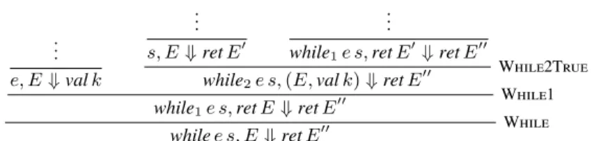
Putting it all together, Figure 1 depicts a full derivation of one run of a loop, where k̸= 0.
The set of terms for our language is defined in Figure 2a. Terms
tare either expressions e, extended expressions ex, statements s,
or extended statements sx. (Ordinary) expressions and statements
form the standard While language, with an added abort statement
abort . An example of an extended expression is +1e2that indi-cates the left expression of + e1e2has been computed, and it is now
the turn of e2to be computed. An example of an extended statement
is if1s1s2that indicates the expression forming the condition has
been evaluated; and the statement to evaluate depends on that result, present in the semantic context.
Evaluation of terms uses the following semantic domains.
•val = Z; •error ={Err};
•env = var→f val, the finite maps from var to val; •oute=val + error, the expression outputs; •outs=env + error, the statement outputs.
Thus, the evaluation of an expression or an extended expression will either produce a value v∈ val or produce an error. Evaluation of a
statement or an extended statement will produce a new environment or an error. To differentiate between a value element of outeand a
value of val, the former will be noted val v and the latter simply v. We proceed similarly for environments, where ret E∈ outs.
.. . e, E⇓ val k .. . s, E⇓ ret E′ .. .
while1e s,ret E′⇓ ret E′′
while2e s, (E,val k)⇓ ret E′′ While2True while1e s,ret E⇓ ret E′′ While1
while e s, E⇓ ret E′′ While
Figure 1: PBS reduction of a while loop
The semantic rules are given in Figure 3. To see how the ex-tended terms work, consider the rule Add1(e)for evaluating the
extended expression +1e. Add1(e)
e, E⇓ o +2, (v1, o)⇓ o′
+1e, (E,val v1)⇓ o′
The evaluation of +1eis done with a semantic context comprised
of an environment E and the output of evaluating the first operand. This rule pattern-matches the latter, requiring it to be a value val v1
and extracting the actual value v1. If +1 e is evaluated with a
semantic context of the form (E, Err), then Add1(e) does not
apply. In that case, the rule AbortE (+1e)applies (see Figure 2d),
which propagates the error.
In the case there was no error, the semantics follows rule Add1(e)and evaluates e to obtain an output for the second operand.
It then constructs another extended expression +2and evaluates it
with a semantic context that includes the value v1the output o.
If this output o is an error, only the rule AbortE (+2)applies
and the error is propagated. Otherwise, the rule Add2applies. Add2
add (v1, v2)⇝ v +2, (v1,val v2)⇓ val v
This rule is called an axiom as none of its premises mention a derivation about⇓. It only performs a local computation, denoted
by⇝, and returns the result.
The PBS format only requires a few rules to propagate errors, even though they may appear at any point in the execution.
3.
Formalization of Rule Schemes
The mechanization of the abstract interpretation of PBS operational semantics is based on a careful analysis of the rule formats used in these semantics. Traditional operational semantics are defined inductively with rules (or, more precisely, rule schemes) of the form
Name
t1, σ1⇓ r1 t2, σ2⇓ r2 . . .
t, σ⇓ r side-conditions
explaining how term t evaluates in a state σ to a result r. There are several implicit relations between the elements of such rule schemes that we make explicit, in order to provide a functional representation for them.
First, we describe the types of the components of t, σ⇓ r. The
first component t is a syntactic term of type term. It is the program being evaluated. The second component σ is a semantic context. It contains the information required to evaluate the program, such as the current state. Its type depends on the term being evaluated: we have σ ∈ st (t). For most terms, the semantic context in our
con-crete semantics is an environment E (see Figure 3). The exceptions are for extended terms that also need information from the previous computations. For instance, the term +1eneeds both an
environ-ment E and a result o as semantic context. Finally, the third compo-nent r is the result of the evaluation of t in context σ. Its type also depends on t: excluding errors, expressions return values whereas instructions return environments. It is written res (t).
Second, rules are identified not only by their name but also by syntactic subterms. For instance, a rule to access the variable x is identified by Var (x), whereas the one for variable y is identified by Var (y). Similarly, a rule for a “while” loop with condition e and body s may be identified by While (e, s). Identifiers are designed such that they uniquely determine the term to which the rule applies. Formally, a PBS semantics carries a set of rule identifiersI and
a function that maps rule identifiers to actual rules (the type Rulei
is described below).
rule : (i∈ I) → Rulei
They also provide a function l that maps rule identifiers to the syntactic term to which the rule applies.
l :I → term
For instance, for the rule Var (x), we have lVar(x)= x.
Third, rules have side-conditions. We impose a clear separation between these conditions and the hypotheses on the semantics of subterms made above the inference line. The conditions involve the rule identifier i and the semantic context σ and are expressed in a predicate cond which states whether rule i applies in the given context σ. For a simple example: two rules can apply to the term x, a variable, depending on whether this variable is defined or not in the given environment E: it is either the look-up rule Var (x) or the error rule VarUndef (x).
Var(x) E[x]⇝ v
x, E⇓ val v x∈ dom(E)
VarUndef(x)
x, E⇓ Err x̸∈ dom(E)
The predicate cond has the type
cond : (i∈ I) → st (li)→ Prop
Finally, the general big-step format allows any number of hy-potheses above the inference line. The pretty-big-step semantics re-stricts this to one of three possible formats: axioms (zero hypothe-ses), rules with one inductive hypothesis, and rules with two in-ductive hypotheses, respectively written Axi, R1,ior R2,ifor a rule
identified by i.
Syntactic Aspects of Rules To summarize, the function type :
I → {Ax, R1,R2} returns the format (axiom, rule 1, or rule 2) of
the rule identified by i∈ I, and l : I → term returns the actual
syntactic term evaluated by a rule. To evaluate a rule, one needs to specify which terms to inductively consider (syntactic aspects) and how the semantic contexts and results are propagated (semantic aspect). We first describe the former.
In format 1 rules, i.e., rules with one hypothesis, the current computation is redirected to the computation of the semantics of another intermediate term (often a sub-term). We thus define a
t ::= e | s | ex | sx e ::= c | x | + e1e2 ex ::= +1e2 | +2 s ::= skip | x := e | s1; s2 | if e s1s2 | while e s | abort sx ::= x :=1 | ;1s2 | if1s1s2 | while1e s | while2e s (a) Terms and Extended Terms
st (e) = env st (s) = env st (+1e2) = env× oute st (+2) = val× oute st (x :=1) = env× oute st (;1s2) = outs st (if1s1s2) = env× oute st (while1e s) = outs st (while2e s) = env× oute (b) Definition of st
The (dependent) type of semantic contexts.
res (ex) = oute res (sx) = outs res (e) = oute res (s) = outs (c) Definition of res The type of results.
abort (Err) = True abort (ret E) = False abort (E, Err) = True abort (E, val v) = False
abort (v, Err) = True abort (v, val v) = False
(d) Definition of abort The abort predicate controls the rules AbortE (ex) and AbortS (sx)of Figure 3.
Figure 2: Concrete Semantics Definitions
AbortE(ex)
ex, σ⇓ Err abort (σ)
AbortS(sx) sx, σ⇓ Err abort (σ) Abort abort , E⇓ Err Cst(c) c, E⇓ val c Var(x) E[x]⇝ v x, E⇓ val v x∈ dom(E) VarUndef(x) x, E⇓ Err x̸∈ dom(E) Add(e1, e2)
e1, E⇓ o +1e2, (E, o)⇓ o′
+ e1e2, E⇓ o′ Add1(e) e, E⇓ o +2, (v1, o)⇓ o′ +1e, (E,val v1)⇓ o′ Add2 add (v1, v2)⇝ v +2, (v1,val v2)⇓ val v Skip skip, E⇓ ret E Asn(x, e) e, E⇓ o x :=1, (E, o)⇓ o′ x := e, E⇓ o′ Asn1(x) E[x7→ v] ⇝ E′ x :=1, (E,val v)⇓ ret E′
Seq(s1, s2) s1, E⇓ o ;1s2, o⇓ o′ s1; s2, E⇓ o′ Seq1(s2) s2, E⇓ o ;1s2,ret E⇓ o If(e, s1, s2) e, E⇓ o if1s1s2, (E, o)⇓ o′ if e s1s2, E⇓ o′ If1True(s1, s2) s1, E⇓ o if1s1s2, (E,val v)⇓ o v̸= 0 If1False(s1, s2) s2, E⇓ o if1s1s2, (E,val v)⇓ o v = 0 While(e, s) while1e s,ret E⇓ o while e s, E⇓ o While1(e, s) e, E⇓ o while2e s, (E, o)⇓ o′ while1e s,ret E⇓ o′ While2True(e, s) s, E⇓ o while1e s, o⇓ o′ while2e s, (E,val v)⇓ o′ v̸= 0
While2False(e, s)
while2e s, (E,val v)⇓ ret E v = 0
Figure 3: Concrete Semantics
function u1 : (i∈ I) → (type (i) = R1) → term returning this
term. Note how this function is restricted on format 1 rules. Similarly, format 2 rules have two inductive hypotheses, hence need to evaluate the semantics of two terms, respectively given by functions u2 : (i ∈ I) → (type (i) = R2) → term and
n2: (i∈ I) → (type (i) = R2)→ term.1
The functions type, l, u1, u2, and n2 describe the structure of
a rule, but not how it computes with the semantic contexts. This computation is done in the transfer functions that are contained in the constructions of type Rulei.
Semantic Aspects of Rules We now define how semantic contexts and results are manipulated according to the semantics. To this end, we define transfer functions, which depend on the format of rule
1u
kstands for “up” and n2stands for “next”.
we are defining. They can be summed up in the following informal scheme, detailed below.
σ1 ⇓ r2 σ4 ⇓ r5 σ3 ⇓ r5 σ0 ⇓ r5 ax ax up up next
Depending on the format of a rule i, Ruleiwill have different
transfer functions. In every case, it will take a semantic context σ of type st (li)and a proof of condi(σ). Depending on the type type (i)
of the rule, it then proceeds as follows to obtain the semantics of t in context σ.
•Axioms directly return a value of type res (li), and are thus
described by a function of type
ax : (σ∈ st (li))→ condi(σ)→ res (li)
Let r∈ res (lId)be the result of an axiom Id for input t∈ term, σ ∈ st (lId), and a proof π of condId(σ). We write such a rule
as follows.
Id
ax (σ, π)⇝ r
lId, σ⇓ r condId(σ)
•Rules with one inductive hypothesis are of the following form.
Id
u1,Id,up (σ)⇓ r
lId, σ⇓ r condId(σ)
Such a rule specifies a new term u1,Idas described above, as well
as a new semantic context up (σ) of type st (u1,Id)and returns
the result of evaluating u1,Id in this context as the semantics
of lId. For such rules, the format thus implicitly requires that res (lId) = res (u1,Id). Hence, the essence of a format 1 rule is the function up that maps σ to up (σ). Together with the
cond predicate and the l and u1 functions, this function up is the only information needed for completely defining such rules. A format 1 rule identified by i is therefore characterized by a function of type
up : (σ∈ st (li))→ condi(σ)→ st (u1,i)
•Rules with two inductive hypotheses are of the following form.
Id
u2,Id,up (σ)⇓ r n2,Id,next (σ, r)⇓ r′
lId, σ⇓ r′ condId(σ)
Such rules first do an inductive call as in the previous case. The result r of this call is then used to build the semantic context for the second inductive call. As the final result is propagated as-is, the required information is: a first semantic context up (σ)∈
st (u2,Id), and a function next (σ,·) transforming the result of the first inductive call into a semantic context of type st (n2,Id).
A format 2 rule i thus consists of two transfer functions:
up : (σ∈ st (li))→ condi(σ)→ st (u2,i)
next : (σ∈ st (li))→ condi(σ)→ res (u2,i)→ st (n2,i) Analogous to rules of format 1, we impose the result type of li
to be that of n2,i, i.e., res (li) =res (n2,i).
To sum up, we define the set of rules as the set Ruleiwhere each
element is one is one of the following.
Axi(ax : (σ∈ st (li))→ condi(σ)→ res (li))
R1,i(up : (σ∈ st (li))→ condi(σ)→ st (u1,i))
R2,i
( up : (σ∈ st (li
))→ condi(σ)→ st (u2,i)
next : (σ∈ st (li))→ condi(σ)→ res (u2,i)→ st (n2,i) )
4.
Mechanized PBS Semantics
We now describe how we implemented this formalization in Coq. The structural aspects directly follow the approach given in the pre-vious section. Assuming a set of terms, we first define the structural part of rules, corresponding to the u1, u2, and n2 functions. They
carry the terms that need to be reduced in inductive hypotheses.
Inductive Rule_struct term := | Rule_struct_Ax : Rule_struct term
| Rule_struct_R1 : term → Rule_struct term
| Rule_struct_R2 : term → term → Rule_struct term.
Id lId, σ⇓ ax (σ) condId(σ) Id u1,Id,up (σ)⇓ r lId, σ⇓ r condId(σ) Id
u2,Id,up (σ)⇓ r n2,Id,next (σ, r)⇓ r′
lId, σ⇓ r′ condId(σ)
Figure 4: Rule Formats
Rule identifiers (name in the Coq files) are associated with the term reduced by the rule (function l, called left in Coq) and to structural terms. They are packaged together as follows.
Record structure := { term : Type; name : Type;
left : name → term;
rule_struct : name → Rule_struct term }.
A semantics, parameterized by such a structure, is then a type of semantic contexts, a type of results, a predicate to determine whether a rule may be applied, and transfer functions for the rules.
Record semantics := make_semantics { st : Type;
res : Type;
cond : name → st → Prop; rule : name → Rule st res }.
We now detail the components of this semantics, highlighting the differences with Section 3.
Although a definition based on dependent types is very elegant, its implementation in Coq proved to be quite challenging. The typi-cal difficulty we had appeared in format 1 and 2 rules where results are passed without modification from a premise to the conclusion, but whose types change from res (lId)to res (uk,Id). In such contexts
these two types happen to be equal because of the implicit hypothe-ses we enforced in the previous section. However, as usually with dependent types, a lot of predicates require these terms to have a specific (syntactical) type. Rewriting “equal” terms (i.e., equal un-der heterogeneous, or “John Major’s”, equality [14]) becomes really painful when there exist such syntactic constraints.
We thus switched to a simpler approach. First, the type for se-mantic contexts (respectively results) is no longer specialized by (or dependent on) the term under consideration: it is the union of every possible semantic context (respectively of every result). This can be seen in the st and res fields above that are simple types.
The rules are then adapted to this setting. They are very similar to the version of Section 3 as can be seen in Figure 4. The Rule type uses the following transfer functions.
Inductive Rule st res :=
| Rule_Ax : (st → option res) → Rule st res | Rule_R1 : (st → option st) → Rule st res | Rule_R2 : (st → option st) →
(st → res → option st) → Rule st res.
The function ax : st → option res for axioms returns None if
the rule does not apply, either because the semantic context does not have the correct shape, or if the condition to apply the rule is
not satisfied. This is in contrast to the definition of Section 3, where the option was not required: the type (σ∈ st (li))→ condi(σ)→
res (li)did guarantee that the semantic context was compatible with the term and that the rule applied.
The transfer function of a format 1 rule is of the form up : st→ option st, constructing a new semantic context if the context given
as argument has the correct shape.
The transfer functions of a format 2 rule are of the form up :
st→ option st and next : st → res → option st.
It may seem that we compute the same thing twice: condi(σ)
states that a given rule i applies to σ, while ax (or the corresponding transfer function) should also return None if the rule cannot be applied. We actually relax this second requirement to allow for simpler definition: transfer functions may return a result even if they do not apply. For instance, the transfer function of VarUndef (x) always returns Err, but it may only be applied if the variable is not in the environment. This separation between side-conditions and transfer functions is a separation between the control flow and the actual computation. In the Coq development, the first one is implemented using predicates, and the second using computable functions.
We now describe how to assemble rules to build a concrete eval-uation relation⇓ ∈ P (term × st × res). We define the concrete
semantics as the least fixed point of a functionF which we now
detail.
F : P (term × st × res) → P (term × st × res)
Given an existing evaluation relation⇓0∈ P (term × st × res), the application function applyi(⇓0) : P (term × st × res) for
rule (i) is as follows. applyi(⇓0) :=
match rule (i) with
| Ax (ax) ⇒ {(li, σ, r)| ax (σ) = Some(r)} | R1(up) ⇒ { (li, σ, r) up (σ) = Some(σ′) ∧ u1,i, σ′⇓0r } | R2(up, next)⇒ (li, σ, r) up (σ) = Some(σ′) ∧ u2,i, σ′⇓0r1 ∧ next (σ, r1) =Some(σ′′) ∧ n2,i, σ′′⇓0Some(r) This relation applyi(⇓0)accepts a tuple (t, σ, r) if it can be com-puted by making one semantic step using rule (i), calling back⇓0
for every recursive call.
The final evaluation relation is then computed step by step us-ing the functionF, computing from an evaluation relation ⇓0the following new relationF (⇓0):
F (⇓0) ={(t, σ, r) | ∃i, condi(σ)∧ (t, σ, r) ∈ applyi(⇓0)} Intuitively, each application ofF extends the relation ⇓0by com-puting the results of derivations with an extra step.
We can equip the set of evaluation relationsP (term × st × res)
with the usual inclusion lattice structure. In this lattice, the functions
applyiandF are monotonic. We can thus define the fixed points of F in this lattice. We consider as our semantics the least fixed point ⇓lfp, which corresponds to an inductive interpretation of the rules: only finite behaviors are taken into account, and no semantics is given to non-terminating programs. We note it⇓.
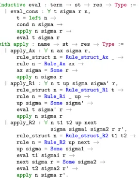
The implementation in Coq shown in Figure 5 directly builds the fixed point as an inductive definition.
Inductive eval : term → st → res → Type := | eval_cons : ∀ t sigma r n,
t = left n →
cond n sigma →
apply n sigma r →
eval t sigma r
with apply : name → st → res → Type := | apply_Ax : ∀ n ax sigma r,
rule_struct n = Rule_struct_Ax _ →
rule n = Rule_Ax ax →
ax sigma = Some r →
apply n sigma r
| apply_R1 : ∀ n t up sigma sigma' r, rule_struct n = Rule_struct_R1 t →
rule n = Rule_R1 _ up →
up sigma = Some sigma' →
eval t sigma' r →
apply n sigma r
| apply_R2 : ∀ n t1 t2 up next
sigma sigma1 sigma2 r r', rule_struct n = Rule_struct_R2 t1 t2 →
rule n = Rule_R2 up next →
up sigma = Some sigma1 →
eval t1 sigma1 r →
next sigma r = Some sigma2 →
eval t2 sigma2 r' →
apply n sigma r'.
Figure 5: Coq definition of the concrete semantics⇓
5.
Mechanized PBS Abstract Semantics
The purpose of mechanizing the PBS semantics is to facilitate the correctness proof of static analyzers with respect to a concrete se-mantics. We thus provide a mechanized way to define an abstract semantics and prove it correct with respect to the concrete one. Its usage to prove static analyzers is described in Section 6.
As stated in the Introduction, the starting point for our develop-ment is the abstract interpretation of big-step semantics, laid out by Schmidt [20]. In this section, we describe how an adapted version of Schmidt’s framework can be implemented using the Coq proof assistant. There are several steps in such a formalization:
•define the Galois connection that relates concrete and abstract domains of semantic contexts and results;
•based on the Galois connection between concrete and abstract domains, prove the local correctness: the side-conditions and transfer functions of each concrete rule are correctly abstracted by their abstract counterpart;
•given the local correctness, prove the global correctness: the abstract semantics⇓♯is a correct approximation of the concrete
semantics⇓, i.e., the least fixed point of the F operator.
The Galois connections relate the concrete and abstract semantic triples (t, σ, r) and(t, σ♯, r♯)by a concretisation function γ. They
let us state and prove the following property relating the concrete and the abstract semantics. Let t∈ term, σ ∈ st, σ♯∈ st♯, r∈ res
and r♯∈ res♯, if σ∈ γ ( σ♯ ) t, σ⇓ r t, σ♯⇓♯r♯ then r∈ γ(r♯ ) .
We illustrate the development through the implementation of a sign analysis for our simple imperative language. However, we emphasize that the approach is generic: once an abstract domain is
⊤ ⊤error ⊤val ± +0 −0 0 + − ⊥
Figure 6: The Hasse diagram of the valerr♯lattice
given, and abstract transfer functions are shown to be correct, then the full abstract semantics is correct by construction.
5.1 Abstract Domains
The starting point for the abstract interpretation of big-step seman-tics is a collection of abstract domains, related to the concrete se-mantic domains by a Galois connection, or just by a concretisa-tion funcconcretisa-tion γ. The formalizaconcretisa-tion of Galois connecconcretisa-tions in proof assistants has been studied in previous work by several authors (e.g., [5, 18]), and we have relied on existing libraries of construc-tors for building abstract domains.
For our example analysis, we have abstracted the base domain of integers by the abstract domain of signs. The singleton domain of errors is abstracted to a two-point domain where⊥errormeans absence of errors and⊤errormeans the possible presence of an error. The result of an expression is either a value or an error, modeled by the sum domain oute. We abstract this by a product domain
with elements of the form(v♯, e♯), where v♯is a property of the
result (if any is produced) and e♯indicates the possibility of an
error. A result that is known to be an error is thus abstracted by (⊥val,⊤error)∈ out♯e. To summarize, the analysis uses the following
abstract domains:
•val♯
=sign ={⊥val,−, 0, +, −0,±, +0,⊤val}; •error♯
={⊥error,⊤error}, named aErr in the Coq files;
•valerr♯=(val♯⊗ error♯)⊤; •env♯
=var→ valerr♯, aEnv in Coq; •out♯
e=val♯× error♯, aOute in Coq; •out♯
s=env♯× error♯, aOuts in Coq.
As the absence of variable in a concrete environment leads to a dif-ferent rule than a defined variable whose value we know nothing about, we have to track the absence of variable in abstract environ-ments. We use the valerr♯lattice to achieve this. Its lattice structure
is pictured in Figure 6. Notice that⊥valand⊥errorare coalesced in this domain, i.e., we construct valerr♯as the smash product of val♯
and error♯.
In the Coq formalization, the discrimination between the possi-ble output domains is implemented with a coalescing sum of partial orders that identifies the bottom elements of the two domains
(
out♯ e+out♯s
)⊤ ⊥
where the new top element indicates a type error due to confusion of expressions and statements. The abstract result type is defined as follows in Coq.
Inductive ares : Type := | ares_expr : aOute → ares | ares_prog : aOuts → ares | ares_top : ares
| ares_bot : ares. 5.2 Rule Abstraction
The abstract interpretation of the big-step semantics produces a new set of inference rules where the semantic domains are replaced by their abstract counterparts. Thus, rules no longer operate over values but over properties, represented by abstract values. For instance, the rule for addition Add2, which applies when both sub-expressions of
an addition have been evaluated to an integer value,
Add2
add (v1, v2)⇝ v +2, (v1,val v2)⇓ val v is replaced by a rule using an abstract operator add♯
Add♯2 add♯
(v1, v2)⇝ v
+2, (v1,val♯v2)⇓♯v
where the concrete addition of integers has been replaced with its abstraction over the abstract domain of signs.
As explained by Schmidt [20, Section 8], the abstract interpre-tation of a big-step semantics must be built such that all concrete derivations are covered by an abstract counterpart. Here, “covered” is formalized by extending the correctness relation on base domains and environments to derivation trees. A concrete and an abstract derivations ∆ and ∆♯are related if the conclusion statement of ∆
is in the correctness relation with the conclusion of ∆♯, and,
fur-thermore, for each sub-derivation of ∆, there exists a corresponding abstract sub-derivation of ∆♯which covers it.
There are several ways in which coverage can be ensured. One way is to add a number of ad hoc rules. For example, it is common for inference-based analyses to include a rule such as
If-abs
Γ⊢ e1: ϕ1 Γ⊢ e2: ϕ2
Γ⊢ if b then e1else e2: ϕ1⊔ ϕ2
that covers execution of both branches of an if.
Instead of adding extra rules, we pursue an approach where we obtain coverage in a systematic fashion, by
1. abstracting the conditions and transfer functions of the individ-ual rules according to a common correctness criterion; 2. defining the way that a set of abstract rules are applied when
analyzing a given term. This is described in Section 5.3 below. We use exactly the same framework (as shown in the Coq develop-ment) for concrete and abstract rules. The only difference is how we assemble abstract rules to build an abstract semantics⇓♯.
Recall that a rule comprises a side-condition that determines if it applies and one or more transfer functions to map the input state to a result. The abstract side-condition cond♯must satisfy the following
correctness criterion. ∀σ, σ♯ . σ∈ γ(σ♯)⇒ cond (σ) ⇒ cond♯ ( σ♯ ) .
Intuitively, this means that whenever there is a state in the concreti-sation of an abstract state σ♯that would trigger a concrete rule, then
the corresponding abstract rule is also triggered by σ♯. Figure 7 is
a snippet from the Coq formalization showing the conditions of the various rules for while. They correspond in a one-to-one fashion to the rules of the concrete semantics defining the cond predicate.
Definition acond n asigma : Prop :=
match n, asigma with
... | name_while e s, ast_prog aE ⇒ True | name_while_1 e s, ast_while_1 ar ⇒ ares_prog (⊥) ⊑ ar | name_abort_while_1 e s, ast_while_1 ar ⇒ ares_prog (⊥,⊤) ⊑ ar | name_while_2_true e s, ast_while_2 aE o ⇒ ares_expr (Sign.pos,⊥) ⊑ o ∨
ares_expr (Sign.neg,⊥) ⊑ o
| name_while_2_false e s, ast_while_2 aE o ⇒
ares_expr (Sign.zero,⊥) ⊑ o
| name_abort_while_2 e s, ast_while_2 aE ar ⇒
ares_expr (⊥,⊤) ⊑ ar
...
Figure 7: Snippet of the cond♯predicate
Definition arule n : Rule sign_ast sign_ares :=
match n with ... | name_while e s ⇒ let up := if_ast_prog (fun E ⇒ Some (sign_ast_while_1 (sign_ares_stat (E, ⊥)))) in Rule_R1 _ up | name_while_1 e s ⇒ let up :=
if_ast_while_1 (fun E err ⇒
Some (sign_ast_prog E)) in let next asigma ar :=
if_ast_while_1 (fun E err ⇒
Some (sign_ast_while_2 E ar)) asigma in Rule_R2 up next
...
Figure 8: Snippet of the rule function
Similar correctness criteria apply to the transfer function defin-ing the rules. For example, axioms, that are defined by a function ax from input states to results, have an abstraction ax♯that must satisfy
∀σ, σ♯ . σ∈ γ ( σ♯ ) ⇒ ax (σ) ∈ γ(ax♯( σ♯ )) .
These criteria are defined as a relation ∼ between rules (called
propagates in the Coq files), made precise below. We assume it has been shown to hold for every pair of concrete and abstract rules sharing the same identifier.
The Coq snippet of Figure 8 shows the encoding of the abstract rules While (e, s) and While1 (e, s). The former is a format 1 and thus only need an up function to be defined. The facts that it applies on lWhile(e,s) =while e s and that its intermediate term is
u1,While(e,s)=while1e sare already expressed by the structure part
and are not shown here.
This function up should be called on a context σ♯that satisfies cond♯
While(e,s)
(
σ♯), that is, on an environment. There is however no typing rule that enforces this (as we do not use dependent types in this formalization, as explained in Section 4) and we thus have to
check this, returningNoneotherwise. We use the following monad to extract the relevant environment.
if_ast_prog :
(aEnv → option sign_ares)
→ sign_ast → option sign_ares
We then compute the semantic context corresponding to u1 = while1e s. In this case, it is sign_ast_while_1 (E, ⊥), where
Eis the extracted environment, as the corresponding rule does not introduce errors while propagating the environment.
The abstract rule While1 (e, s) is a format 2 rule and thus needs two functions, up and next, to be similarly defined. As the expected kind of the semantic context is in this case the one of while1e s, we
use a different monad:
if_ast_while_1 :
(aEnv → aErr → option sign_ares)
→ sign_ast → option sign_ares
These definitions are so similar to the concrete definitions that they can be built directly from a concrete definition. This similarity simplifies definitions and proofs considerably.
Finally, the relation∼ that relates concrete and abstract rules can
be defined as follows.
•A concrete and an abstract axioms ax : st → res and ax♯
:
st♯ → res♯ are related iff for all σ and σ♯ on which both
functions ax and ax♯ are defined, and such that σ ∈ γ( σ♯), then ax (σ)∈ γ(ax♯(σ♯)).
•A concrete and an abstract format 1 rules up : st → st and up♯
: st♯ → st♯are related iff for all σ and σ♯on which both
functions up and up♯are defined, and such that σ∈ γ( σ♯), then
up (σ)∈ γ(up♯(σ)).
•For format 2 rules, we impose the same condition on the up and up♯transfer functions than above, and we add the additional
condition over the transfer functions next : st→ res → st and
next♯
:st♯→ res♯→ st♯: for all σ, σ♯, r and r♯on which both
functions next and next♯are defined, and such that σ∈ γ( σ♯)
and r∈ γ(r♯), then next (σ, r)∈ γ(next♯(σ♯, r♯)). 5.3 Inference Trees
Concrete and abstract semantic rules have been defined to have similar structure. However, the semantics given to a set of abstract rules differs from the concrete semantics defined in Section 4. This difference manifests itself in the way rules are assembled.
First, the function apply♯
ifor applying an abstract rule with
iden-tifier i extends the applyifunction by allowing to weaken semantic contexts and results. Indeed, the purpose of the abstract semantics is to capture every correct abstract analyses, including the ones that lose precision. It is thus possible to choose a less precise seman-tic context σ0 before referring to applyi, and to then return a less
precise result r afterwards.
apply♯ i ( ⇓♯ 0 ) = (t, σ, r) ∃σ0,∃r0, σ⊑♯σ0∧ r0⊑♯r∧ (t, σ0, r0)∈ applyi ( ⇓♯ 0 ) Second, we define a functionF♯that infers new derivations from
a set of already established derivations, by applying the abstract inference rules. The definition of the functionF♯differs in one
important aspect from its concrete counterpart: in order to obtain coverage of concrete rules,F♯ must apply all the rules that are
Var(x) x,{x 7→ +0} ⇓♯+0 ·· ·· ·· ·· ·· ·· ·· ·· ·· while2x s, ({x 7→ +0} , +0)⇓♯{x 7→ +0}While2False(x, s) s,{x 7→ +0} ⇓♯{x 7→ ⊤val} . ..
while1x s,{x 7→ ⊤val} ⇓♯{x 7→ ⊤val} While1(x, s) while2x s, ({x 7→ +0} , +0)⇓♯{x 7→ ⊤val} While2True(x, s)
while1x s,{x 7→ +0} ⇓♯{x 7→ ⊤val} While1(x, s) while x s,{x 7→ +0} ⇓♯{x 7→ ⊤val} While(x, s)
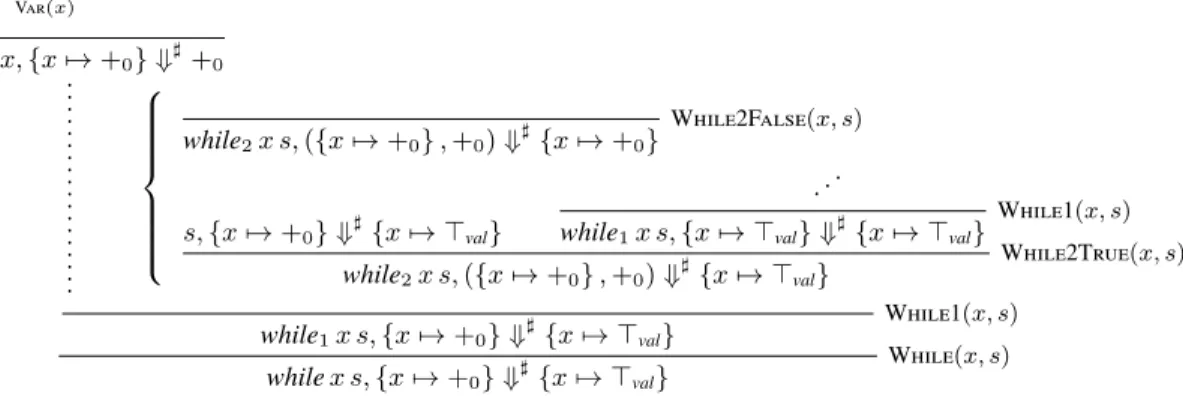
Figure 9: An infinite abstract derivation tree corresponding to a finite concrete derivation tree, where s≜ (x := + x (−1))
enabled for a term in the given abstract state.
F♯(⇓♯ 0 ) = { (t, σ, r) ∀i. t = li⇒ condi(σ)⇒ (t, σ, r)∈ apply♯i ( ⇓♯ 0 ) }
In other words, the function extends the relation⇓♯
0by adding those
triples (t, σ, r) such that the result r is valid for all rules. By defining
F♯in this way, we avoid having to add rules such as the If-abs rule
from above: a correct result is one that includes the computation from both branches.
Let us consider a simple example to give some intuition. The program if x (r := 0) (r := x) always sets r to zero if x is defined. Let us analyze it in an environment E♯
1 ∈ env
♯where x is +, and
in an environment E♯ 2 ∈ env
♯ where x is⊤val, i.e., x is defined
but we know nothing about its value. In either case, it expands after one step to if1 (r := 0) (r := x), and carries an information about
the computed expression x that is either + or⊤val(or any weaker result, but we only consider a precise derivation in this example). In the first case we know that this expression is non zero, and only the rule If1True (r := 0, r := x) applies: we evaluate r := 0 and can conclude that r is zero. However in the second case, we don't know which branch will be executed and thus additionally consider the rule If1False (r := 0, r := x). This branch executes r := x and sets r to⊤val. This example illustrates a shortcoming of our approach: even though we know the value tested has to be 0 in the “false” branch, there is no information about how that value was computed (evaluating x in this example). The non-local information that allows to deduce that x is bound to 0 in the environment is currently not available to our framework.
The functionF♯is a monotone function on the lattice P(term× st♯× res♯)
.
The least fixed point ofF♯(with respect to the inclusion⊆ order)
corresponds to all triples that can be inferred using finite derivation trees. These triples are valid properties of the program, but the restriction to finite derivations means that certain properties cannot be inferred.
Consider the program while x (x := + x (−1)) evaluated on a
context where x is positive. Its concrete derivation clearly termi-nates, but there is no finite derivation in the sign abstraction seman-tics to witness it. Indeed, initially x is bound to +0. After the first
iteration, it is bound to⊤val, then its value becomes stable. Every subsequent iteration thus has to consider the case where x is not 0and to compute an additional iteration. Hence, there is no finite abstract derivation: the abstract domain is not precise enough.
Intuitively, since the concrete derivation tree has to be “in-cluded” into the abstract derivation tree, and since there is no bound
on the number of execution steps in the concrete derivation (which depends on the initial value of x, the loop being unfolded that many times), any abstract derivation has to be infinite.
Figure 9 depicts the abstract derivation tree built by recur-sively applyingF♯, writing s for (x := + x (−1)). Both rules
While2True (x, s) and While2False (x, s) are executed and their results{x 7→ +0} and {x 7→ ⊤val} are merged (in this case, the
sec-ond merged element is greater than the first one). This follows the definition ofF♯, that applies every rule that can be applied.
We thus need to allow infinite abstract derivations. To this end, the abstract evaluation relation, written⇓♯, is obtained as the
great-est fixed point of F♯. The correctness of this extension, since lfp(F♯) ⊆ ⇓♯, has been proven in Coq. More importantly, a
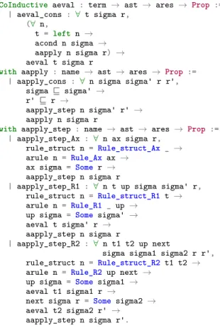
co-inductive approach allows analyzers to use more techniques, such as invariants, to infer their conclusions. The snippet of Figure 10 shows the definition of⇓♯in Coq. Note the symmetry between this
definition and the concrete definition of⇓ in Figure 5. 5.4 Correctness of the Abstract Semantics
We have defined the local correctness as the conjunction of the correctness of the side-condition predicates cond and cond♯and the
correctness of the transfer functions∼, whose Coq versions follow:
Hypothesis acond_correct : ∀ n asigma sigma,
gst asigma sigma → cond n sigma → acond n asigma.
Hypothesis Pr : ∀ n, propagates (arule n) (rule n).
We proved in Coq that under the local correctness, the concrete and abstract evaluation relations,
⇓ = lfp (F) ⇓♯
= gfp(F♯)
are related as follows.
Theorem 1 (Correctness). Let t∈ term, σ ∈ st, σ♯∈ st♯, r∈ res and r♯∈ res♯. If σ∈ γ ( σ♯ ) t, σ⇓ r t, σ♯⇓♯r♯ then r∈ γ(r♯ ) .
Here follows the Coq version of this theorem. It has been proven in a completely parameterized way with respect to the concrete and abstract domains, as well as the rules.
CoInductive aeval : term → ast → ares → Prop := | aeval_cons : ∀ t sigma r, (∀ n, t = left n → acond n sigma → aapply n sigma r) → aeval t sigma r
with aapply : name → ast → ares → Prop := | aapply_cons : ∀ n sigma sigma' r r',
sigma ⊑ sigma' →
r' ⊑ r →
aapply_step n sigma' r' →
aapply n sigma r
with aapply_step : name → ast → ares → Prop := | aapply_step_Ax : ∀ n ax sigma r,
rule_struct n= Rule_struct_Ax _ →
arule n = Rule_Ax ax →
ax sigma = Some r →
aapply_step n sigma r
| aapply_step_R1 : ∀ n t up sigma sigma' r, rule_struct n= Rule_struct_R1 t → arule n = Rule_R1 _ up →
up sigma = Some sigma' →
aeval t sigma' r→
aapply_step n sigma r
| aapply_step_R2 : ∀ n t1 t2 up next
sigma sigma1 sigma2 r r', rule_struct n= Rule_struct_R2 t1 t2 →
arule n = Rule_R2 up next →
up sigma = Some sigma1 →
aeval t1 sigma1 r →
next sigma r = Some sigma2 →
aeval t2 sigma2 r' →
aapply_step n sigma r'.
Figure 10: Coq definition of the abstract semantics⇓♯
Theorem correctness : ∀ t asigma ar, aeval _ _ _ t asigma ar → ∀ sigma r,
gst asigma sigma → eval _ t sigma r → gres ar r.
The predicates aeval and eval respectively represent⇓♯and⇓,
while gst and gres are the concretisation functions for the seman-tic contexts and the results.
This allows us to easily prove the correctness of an abstract semantics with respect to a concrete semantics. We now show how this abstract semantics can be related to analyzers.
6.
Building Certified Analyzers
The abstract semantics⇓♯is the set of all triples provable using the
set of abstract inference rules. From a program t and an abstract se-mantic context σ♯, the smallest r♯such that t, σ♯⇓♯
r♯corresponds to the most precise analysis. It is, however, rarely computable. De-signing a good certified analysis thus amounts to writing a program that returns a precise result that belongs to the abstract semantics.
To this end, we heavily rely on the co-inductive definition of⇓♯
to prove the correctness of static analyzers. In order to prove that a given analyzerA : term → st♯ → res♯is correct with respect to ⇓♯, (and thus with respect to the concrete semantics by Theorem 1),
it is sufficient to prove that the set
⇓♯ A= {( t, σ♯,A ( t, σ♯ ))} is coherent, that is⇓♯ A ⊆ F♯ ( ⇓♯ A )
. Alternatively, on may define for every t and σ♯a set R
t,σ♯ ∈ P
(
term× st♯× res♯)such that
( t, σ♯,A ( t, σ♯ )) ∈ Rt,σ♯and Rt,σ♯ ⊆ F♯ ( Rt,σ♯ ) . This is exactly Park’s principle [17] applied toF♯.
We instantiate this principle in Coq through the following alter-native definition of⇓♯
. The parameterized predicate aeval_check applies one step of the reduction: it exactly corresponds toF♯and
is defined in Coq similarly to aeval (Figure 10). More precisely, aeval is the co-inductive closure of aeval_check; we do not de-fine it directly as such because Coq cannot detect productivity.
Inductive aeval_f : term → ast → ares → Prop := | aeval_f_cons : ∀ (R : term → ast → ares → Prop)
t sigma r, (∀ t sigma r, R t sigma r → aeval_check R t sigma r) → R t sigma r → aeval_f t sigma r.
We then show the equivalence theorem that allows us to use Park’s principle.
Theorem aevals_equiv : ∀ t sigma r, aeval t sigma r ↔ aeval_f t sigma r.
Using this principle, we have built and proved the correctness of several different analyzers, available in the Coq files accompanying this paper [4]. Most of these analyzers are generic and can be reused as-is2 with any abstract semantics built using our framework. We
next describe two such analyzers.
•Admitting a⊤ rule as a trivial analyzer that always return ⊤
independently of the given t and σ♯.
•Building a certified program verifier that can check loop invari-ants from a (non-verified) oracle and use these to make abstract interpretations of programs.
Admitting a⊤ rule This trivial analyzer shows how to add derived
rules to the abstract semantics. There is indeed no axiom rule that directly returns the⊤ result for any term and context. Admitting this rule (which is often taken for granted) amounts exactly to prove that the corresponding trivial analyzer is correct. We thus define the set⇓♯
⊤ =
{(
t, σ♯,⊤)}and prove it coherent. We have to prove that every triple(t, σ♯,⊤) is also part ofF♯(⇓♯
⊤
)
, that is that for every rule i that applies, i.e., cond♯
i ( σ♯), then(t, σ♯,⊤) ∈ apply♯ i ( ⇓♯ ⊤ )
. But as⊤ is greater than any other result, we just have to prove that there exists at least one result r♯such that(t, σ♯, r♯)∈ apply♯ i ( ⇓♯ ⊤ )
. This last property is implied by semantic fullness, which we require for every semantics: transfer functions are defined where cond♯holds.
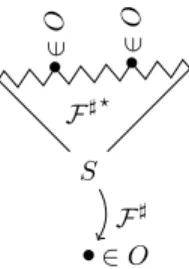
Building a certified program verifier To allow the usage of ex-ternal heuristics to provide potential program properties, and thus relax proof obligations, we have also proved a verifier: it takes an oracle, i.e., a set of triples O∈ P(term× st♯× res♯), and accepts
or rejects it. An acceptance implies the correctness of every triple
2A function computing the list of rules which apply to a given t and σ♯has to be defined. Some of these generic analyzers also need a function detecting “looping” terms (in this example terms of the form while1s1s2).
• ∈ O S F♯ F♯⋆ •∈ O •∈ O
Figure 11: An Illustration of the Action of the Verifier
of O. For every triple o =(t, σ♯, r♯)∈ O, the verifier checks that
it can be deduced from finite derivations starting from axioms and elements of O, i.e., O ⊆ F♯+(O). In practice, the verifier
com-putes hypotheses that imply o, a subset S ofF♯−1
(o)such that
o∈ F♯+(S), and it iterates on S recursively until it reaches only elements of O and axioms, or until it gives up. This is illustrated in Figure 11. We prove the following.
Theorem 2 (Correctness of the verifier). If the verifier accepts O, then O⊆ F♯+
(O)hence O⊆ ⇓♯.
We extracts the verifier into OCaml. Note that it can be given any set, possibly incorrect. In that case it will simply give up. We have tested the verifier on some simple sets of potential program properties. These sets were constructed by following some abstract derivation trees up to a given number of loop unfoldings and ignor-ing deeper branches.
As an example, consider this program that computes 6×7 using
a while loop.
a := 6; b := 7; r := 0; n := a;while n (r := + r b; n := + n (−1))
Using our analyzer on this program in the environment mapping every variable to⊤errorreturns the following result.
({r 7→ +, b 7→ +, a 7→ +, n 7→ ⊤val} , ⊥)
This means that we successfully proved that the program does not abort (i.e., it does not access an undefined variable), but also that the returned value is strictly positive (i.e., the loop is executed at least once). Note that this is the best result we can get on such an example with this formalism and the sign abstract domains. In particular, remark that the sign domain cannot count how many times the loop needs to be unfolded, hence the abstract derivation is infinite. Nevertheless, the analysis deduces significant information.
7. Related Work
Schmidt’s paper on abstract interpretation of big-step operational semantics [20] was seminal but has had few followers. The only re-ported uses of big-step semantics for designing a static analyzer are those of [10] who built a big-step semantics-based foundation for program slicing by Gouranton and Le Metayer [10] and of Bagnara
et. al. [1] concerned with building a static analyzer of values and
array bounds in C programs.
Other systematic derivations of static analyses have taken small-step operational semantics as starting point. With the aim of analyz-ing concurrent processes and process algebras, Schmidt [21] dis-cusses the general principles for such an approach and compares small-step and big-step operational semantics as foundations for ab-stract interpretation. Cousot [8] has shown how to systematically derive static analyses for an imperative language using the princi-ples of abstract interpretation. Midtgaard and Jensen [15, 16] used a similar approach for calculating control-flow analyses for functional languages from operational semantics in the form of abstract
ma-chines. Van Horn and Might [22] show how a series of analyses for functional languages can be derived from abstract machines. An ad-vantage of using small-step semantics is that the abstract interpreta-tion theory is conceptually simpler and more developed than its big-step counterpart. In particular, accommodating non-termination is straightforward in small-step semantics. As both Schmidt and later Leroy and Grall [13] show, non-termination can be accommodated in a big-step semantics at the expense of accepting to work with in-finite derivation trees defined by co-induction. Interestingly, the de-velopment of the formally verified CompCert compiler [12] started with big-step semantics but later switched to a mixture of small-step and big-step semantics. Poulsen and Mosses [19] have used refocus-ing techniques to automatically compile small-step semantics into PBS semantics.
Machine-checked static analyzers including the Java byte code verifier by [11] and the certified flow analysis of Java byte code by [6] also use a small-step semantics as foundation. Cachera and Pichardie [5] use denotational-style semantics for building certified abstract interpretations. In spite of the difference in style of the un-derlying semantics, these analyzers rely on the same formalization of abstract domains as lattices. The correctness proof also include similar proof obligations for the basic transfer functions.
In our Coq formalization we have striven to stay as close to Schmidt’s original framework as possible, but there are a few de-viations.
•Our development is based on a specific kind of big-step opera-tional semantics i.e., the PBS rule format. For the formalization, this has the advantage that the rule format becomes precisely defined while still retaining full generality.
•Schmidt also considers infinite derivations for the concrete se-mantics. More precisely, the set of derivation trees is taken to be the greatest fixed point gfp(Φ) of the functional Φ induced by the inference rules. The trees can be ordered so that the set of semantic trees form a cpo, with a distinguished smallest element Ω, denoting the undefined derivation. The semantics of a term t in state E is then defined to be the least derivation tree that ends in a judgment of form t, E⇓ r. This tree can be obtained as the least fixed point of the functionalE : Term → env → gfp(Φ) induced by the inference rules.
•When constructing the abstract semantics, we only abstract conditions and transfer functions of concrete semantic rules. Schmidt’s notion of covering relation between concrete and ab-stract rules is more flexible in that it allows the abab-stract seman-tics to be a completely different set of rules, as long as they can be shown to cover the concrete semantics. Also, we do not in-clude extra meta-rules that can be shown to correspond to sound derivations (such as a fixed point rule for loops and a rule for weakening, for example) in the basic setup. As shown in Sec-tion 6, such meta-rules can be shown to be sound within our framework. This deviation guides the definition of the abstract semantics, helping its mechanization.
•Schmidt appeals to an external equation solver over abstract domains to make repetition nodes in a derivation tree. We show how to use an oracle analyzer to provide loop invariants that are then being verified by the abstract interpreter.
8.
Conclusions and Future Work
Big-step operational semantics can be used to develop certified abstract interpretations using the Coq proof assistant. In this paper, we have described the foundations of a framework for building such abstract interpreters, and have demonstrated our approach by developing a certified abstract interpreter over a sign domain for a While language extended with an exception mechanism. The