HAL Id: hal-01410069
https://hal.inria.fr/hal-01410069
Submitted on 6 Dec 2016
HAL is a multi-disciplinary open access
archive for the deposit and dissemination of
sci-entific research documents, whether they are
pub-lished or not. The documents may come from
teaching and research institutions in France or
abroad, or from public or private research centers.
L’archive ouverte pluridisciplinaire HAL, est
destinée au dépôt et à la diffusion de documents
scientifiques de niveau recherche, publiés ou non,
émanant des établissements d’enseignement et de
recherche français ou étrangers, des laboratoires
publics ou privés.
Fault-Tolerant and Constrained Relay Node Placement
in Wireless Sensor Networks
Ines Khoufi, Pascale Minet, Anis Laouiti
To cite this version:
Ines Khoufi, Pascale Minet, Anis Laouiti. Fault-Tolerant and Constrained Relay Node Placement in
Wireless Sensor Networks. The 13th IEEE International Conference on Mobile Ad hoc and Sensor
Systems (IEEE MASS 2016), Oct 2016, Brasilia, Brazil. �hal-01410069�
Fault-Tolerant and Constrained Relay Node
Placement in Wireless Sensor Networks
Ines Khoufi, Pascale Minet
Centre de Recherche Inria de Paris 2 rue Simone Iff, CS 42112, 75589 Paris Cedex 12, France
Email: [email protected], [email protected]
Anis Laouiti
SAMOVAR, T´el´ecom SudParis CNRS, Universit´e Paris-Saclay, 9 rue Charles Fourier 91011 EVRY, France
Email: [email protected]
Abstract—In this paper we focus on wireless sensor networks deployed to cover some given Points of Interest (PoIs), achieve connectivity with the sink and be robust against link and node failures. The Relay Node Placement problem (RNP) consists in minimizing the number of relays needed and the maximum length of the paths connecting each PoI with the sink. We propose a solution that determines the positions of relay nodes based on the virtual grid computed by the optimal deployment for full area coverage. We compare our solution with two different solutions based respectively on 1) the straight line that builds the shortest path between each PoI and the sink, 2) the Steiner point that connects PoIs together. We then extend these algorithms to achieve k-connectivity. Our solution outperforms the Steiner points solution in terms of maximum path length on the one hand, and the straight line solution in terms of total number of relay nodes deployed on the other hand. We also apply our solution in an area containing obstacles and show that it provides very good performances.
I. CONTEXT ANDMOTIVATIONS
Since the deployment cost of wired networks in in-dustrial environments is very high, not all sources of potential information related to the industrial process have been connected to the wired network even though they would provide very useful information for analyzing and improving the industrial process. That is why a wireless sensor network (WSN) is used to cover some given points of interest (e.g. a leaking valve). The sensor nodes are responsible for sensing their environment (e.g. a flowmeter for a pipe) and transmitting useful data usually in multi-hop manner to a sink for their analysis. It is often necessary to deploy additional wireless nodes to act as relays to ensure connectivity with the sink. Network connectivity is an important challenge in WSNs since several factors may cause the failure of wireless transmissions. On the one hand, wireless communication links may be unstable for many reasons: interferences, multipath propagation and fading to name but a few. On the other hand, sensor nodes may exhaust their source of energy, usually a battery. As a consequence, the wireless sensor network must be able to tolerate link and node failures.
In this paper we focus on wireless sensor networks deployed to cover some given points of interest, achieve connectivity with the sink and be robust against link and node failures. More precisely, we want to minimize the number of relays deployed as well as the maximum length of paths connecting each PoI with the sink. The reason is that the transfer of any message on a longer path consumes more bandwidth and more energy. These resources are limited in a wireless sensor network. Since the reliability of a path is equal to the product of the reliability of each link composing it, a long path is less reliable than a short one, assuming that all links have a similar reliability and links of poor quality are not selected in path building. Hence, to maximize robustness, we will favor short paths from any PoI to the sink. In addition, the end-to-end delivery delay depends on the number of hops involved. That is why short paths are favored, provided that they are able to ensure the quality of service (QoS) required by the application.
This paper is organized as follows. In Section II, we give a brief state of the art related to the coverage of points of interest and connectivity including methods based on Steiner points. We then see how to improve robustness with k-connected networks. In Section III, we formally define the relay node placement problems we study and list our assumptions. In Section IV, assuming no link/node failure, we study three solutions based on heuristics: the Straight Line, the Steiner Point and the Triangular Grid based solutions. We compare them in terms of the number of relay nodes needed, the path length to the sink and the average node degree. In Section V we then improve these solutions to achieve robustness with regard to link and node failures and evaluate their performance. In Section VI, we show how to extend our solution to cope with obstacles. Finally, we conclude in Section VII.
II. STATE OF THEART
The first coverage problem that has been studied in WSNs deals with full area coverage [1]. When the
sens-ing range r and the communication range R of sensor nodes satisfy the following inequation R ≥ r√3, full coverage implies connectivity. The optimal deployment (i.e., the deployment that ensures full area coverage with the minimum number of sensor nodes) is given by an equilateral placement of sensor nodes in the area considered, as proved in [2]. This deployment is optimal under the assumption of a disk based model for radio communication and sensing range. Although this deployment ensures that all the points of interest are covered and guarantees that they are connected to the sink, the number of sensor nodes required may result in a prohibitively high cost. That is why other strategies are preferred to cover PoIs.
To minimize the number of relay nodes (i.e, additional wireless nodes deployed to ensure connectivity with the sink), one strategy consists in using the property of the Steiner point in a triangle. For instance, the algorithm given in [3] builds the minimum Steiner tree on the convex hull of the points of interest. It proceeds iteratively. At each iteration, the algorithm selects the points of interest that have not yet been considered and the Steiner point of the previous iteration (if any), all these points belonging to the outermost convex hull not yet considered. The Steiner point of every three consecutive points of the convex hull is computed. The Steiner points are the optimized locations of the relay nodes. The algorithm stops when all PoIs have been selected. Additional relay nodes are added if necessary (i.e. when the distance is greater than the communication range) on each straight line connecting each PoI to its Steiner point as well as between any Steiner point obtained at iteration i and its Steiner point obtained at iteration i + 1. Many other algorithms based on the Steiner points principle exist in the literature [4].
To tolerate k − 1 failures of wireless links or nodes, k-connectivity has been introduced. The authors of [5] focus on k-connectivity in a WSN while minimizing the number of relay nodes. The solution proposed takes benefit of overlapping node communication areas to place a relay node at the intersection of overlapping communication areas to achieve connectivity. Hence, this relay node is within transmission range of at least two other nodes. We will see in Section VI how this principle is adapted to cope with obstacles.
Another study [6] focuses on the problem of fault tolerant relay nodes placement in heterogeneous wireless sensor networks where sensor nodes and relay nodes have different communication ranges. The authors use the steinerization of edges to create a path between two sensor nodes. The idea is to start by deploying two relay nodes: each relay node is placed at a distance equal to the minimum communication range between
sensor nodes and relay nodes, from each path extremity. Then, additional equidistant relays are added on the remaining path between the two relays deployed. Han et al. [6] formalized the relay node placement problem that minimizes the number of relay nodes deployed to ensure that there exists k ≥ 1 node-disjoint paths between every pair of nodes, a node being a sensor node or the base station. If k > 1, node placement is said fault-tolerant. The authors proposed approximation algorithms to solve these NP-hard problems.
Misra et al. [7] studied the constrained relay node placement, where the relay nodes can only occupy a set of candidate locations and the number of relay nodes needed to connect each sensor node with k = 1 or 2 base station(s) through k node-disjoint paths. If k = 2 the relay node placement is said survivable. Misra et al. [7] propose approximation algorithms to solve these problems.
However, our problem is different: we are interested in ensuring an efficient connectivity between each PoI and the sink. We do not focus on the connectivity between PoIs but want to minimize the length of the paths connecting each PoI with the sink, for efficiency reasons. Misra [7] and Han [6] do not minimize the length of the path of each PoI to the sink, but the total weight of the tree including all PoIs, where the weight between two nodes is equal to the number of relays needed to ensure connectivity between them.
Another strategy comes from bio-inspired networks, where the evolution process of real organisms has natu-rally selected the most robust ones. The idea developed in [8] is to extract from the Gene Regulatory Network (GRN) of living organisms (e.g., yeast and the E. coli bacterium) a subnetwork with the same number of nodes as the number of sensor nodes to deploy and finally to place sensor nodes in a grid such that there is an isomorphism between the edges in the GRN subnetwork and their counterparts in the WSN. The authors show that these bio-inspired networks have very interesting structural properties such as a shorter average path length, a smaller average network diameter and fewer disconnected components to the sink after a random removal of edges, etc. We adopt these metrics for the performance evaluation of our solution. Our solution has structural properties inherited from the grid (i.e. triangu-lar tesselation) providing the optimal deployment [9].
In this paper, we are interested in monitoring PoIs by deploying relay nodes to ensure connectivity be-tween each PoI and the sink. To do so, we propose an algorithm based on the deployment that has been proved optimal for full area coverage and compare its performance with these of Straight-Line and Steiner-Point based algorithms. We also focus on increasing
robustness by ensuring k node-disjoint paths from each PoI to the sink and study how obstacles can be tackled. The presence of obstacles implies that some places are forbidden for the placement of relays. However, this is not the only constraint: two nodes at a distance less than R may be unable to communicate because of the presence of an obstacle between them.
III. RELAYNODEPLACEMENT PROBLEMS
A. Problem definitions
Before defining the Relay Node Placement problems (RNP), we first define our notations.
Let P denote the set of PoIs that must be covered. We have P = {P1, P2, . . . , Pn}, with n ≥ 1.
Let P0 be the sink.
Let R be the communication range of relays and sensor nodes.
Let L(i) be the length of the path of any PoI Pi to the
sink, with i ∈ [1, n].
Let Nrbe the number of relay nodes deployed to ensure
connectivity of each PoI with the sink.
With regard to relay node placement, we distinguish two types of problems:
• The relay node placement, called RNP problem: to minimize the number of relay nodes deployed as well as the maximum length of the paths connecting each PoI to the sink:
min{Nr· maxi∈[1,n]L(i)}. (1)
We define a variant of this problem where relay nodes cannot be placed anywhere: relay node placement is constrained by the presence of obstacles and the border of the area considered. On the one hand, the presence of obstacles constrains the placement of relay nodes: places within an obstacle are forbidden. On the other hand, the presence of obstacles may cause hidden nodes that may break connectivity.
The constrained relay node placement, called C-RNP problem: to minimize the number of relay nodes deployed in an area with obstacles as well as the maximum length of paths connecting each PoI to the sink:
minobstacle{Nr· maxi∈[1,n]L(i)}. (2)
where obstacles are taken into account (e.g. forbidden places and connectivity loss).
• The fault-tolerant relay node placement, called
FT-RNP problem: to minimize the total number of relay nodes deployed as well as the maximum lengths of primary paths and secondary paths connecting each PoI to the sink, respectively: Each PoI is connected to the sink via k node-disjoint paths.
min{Nr· maxi∈[1,n]Lp(i) · maxi∈[1,n]Ls(i)}. (3)
where Lp(i) is the length of the primary path of PoI Pi
to the sink, Ls(i) is the length of the secondary path of PoI Pito the sink and Nrthe total number of relay nodes
deployed to ensure k-connectivity of each PoI with the sink.
Similarly, we can define a variant, where the fault-tolerant relay node placement is constrained by obsta-cles. The constrained fault-tolerant relay node place-ment, C-FT-RNP problem: to minimize the number of relay nodes deployed in an area with obstacles as well as the maximum length of primary paths and secondary paths connecting of each PoI to the sink, respectively:
minobstacle{Nr· maxi∈[1,n]Lp(i) · maxi∈[1,n]Ls(i)}.
(4) where obstacles are taken into account(e.g. forbidden places and connectivity loss).
B. Network model
We assume a disk-based model for radio communi-cation. All nodes, (i.e. relay nodes and sensor nodes) have the same communication range R. Two nodes at a distance less than or equal to R are able to communicate with each other in the absence of obstacles.
Obstacles prohibit the presence of sensor nodes in cer-tain locations and may prevent direct communication between sensor nodes. We distinguish two types of obstacles: opaque and transparent.
• Transparent obstacles, have no impact on both the
sensing range and the communication range of nodes. They only prohibit the presence of nodes.
• Opaque obstacles, like transparent obstacles
pro-hibit the presence of nodes. However, they may prevent the communication between nodes at a distance < R, as seen in Section VI.
IV. RELAYNODEPLACEMENT: RNP
In this section, we assume there is neither link/node failure, nor obstacles. We will see later how to relax these assumptions. We present three solutions based on heuristics: an intuitive solution based on the straight line, a solution based on the Steiner point and finally our proposed solution based on the triangular grid.
A. An intuitive solution: The Straight-Line heuristic The straight-line-based algorithm is the simplest so-lution and the most intuitive one that we propose as a baseline for comparison. It is inspired from a wired classical deployment where each PoI is linked to the sink with a straight line cable. Here we simply propose to cut the wires and deploy a set of relay nodes along that path between each PoI and the sink. This algorithm deploys a relay node every R meters on the straight line binding a PoI to the sink. Hence, each PoI is connected to the sink
by the shortest path, as illustrated in Figure 1 where 14 PoIs are connected to the sink. However, this solution has two main drawbacks. First, it is not robust: on any path to a PoI, the failure of a single node or link disconnects the PoI concerned if there is no neighboring node to bypass the failed node or link. Second, no relay node is shared between PoIs. Hence, the number of relays deployed may be very high.
Fig. 1: The Straight-Line Algorithm for 14 PoIs. B. A solution based on relay sharing: the Steiner-Point
By definition, the Steiner point S of three points A, B and C is the point that minimizes the sum of the distance to the three vertices of the triangle ABC. Hence, by definition of S, we have for any point P , d(A, S) + d(B, S)+d(C, S) ≤ d(A, P )+d(B, P )+d(C, P ), where d(A, B) denotes the euclidean distance between A and B. See Figure 2 for an illustration. Notice that the Steiner point of the three points A, B and C is B itself if the angle (A,B,C) is higher than or equal to 120 degrees.
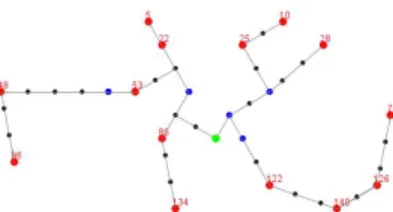
Fig. 2: The Steiner point S of A, B and C. The Steiner-Point-based algorithm builds a path from each PoI represented in red to the sink in green using the closest neighbor which may be another PoI, a Steiner Point in blue or simply a relay node, as illustrated in Figure 3 where 14 PoIs in red are connected to the sink in green. An initial consequence is that this algorithm enables PoIs to share some relay nodes, thereby reducing the total number of relay nodes needed, as we will see in Section IV-D2. The second consequence is that the path from a PoI to the sink may lead further away from the sink before getting closer to the sink, like for instance the path originated at node 78 in Figure 3. This phenomenon is evaluated by the path length from each PoI to the sink in Section IV-D3.
C. Our solution: the Triangular-Grid-Based Algorithm The solution we propose, uses the virtual grid of the deployment proved optimal in [2] and defined in the circumscribing rectangle which includes all the PoIs. In this deployment, nodes are placed according to a trian-gular lattice. We propose to build the shortest path from
Fig. 3: The Steiner-Points-Based Algorithm for 14 PoIs.
each PoI to the sink using only relay nodes belonging to the optimal deployment grid. In the final deployment, only relay nodes that are used by at least one PoI are kept. This solution favors both the sharing of relay nodes between PoIs in red and short paths to the sink in green where relay nodes are represented in blue, as illustrated in Figure 4 where 14 PoIs are connected to the sink. This solution is called Triangular-Grid-Based algorithm. We do not claim that this algorithm provides an optimal deployment but only that it tends to minimize the number of relays deployed as well as the length of the path from any PoI to the sink.
Fig. 4: The Triangular-Grid-Based Algorithm. D. Performance Evaluation
For the performance evaluation of the three solutions previously described, we developed our own simulation tool in Java and implemented the three solutions. The choice of a Java simulation tool is motivated by the need to obtain fast performance results, noticing that these results do not depend on the network communication protocols used by the WSN in question. We consider different configurations where the number of PoIs varies from 15, 30 to 45. For each configuration characterized by a given number of PoIs, we randomly select the position of each PoI (at a distance higher than 2R from the sink) in the area considered which corresponds to a square of size L = 25r, where r is the sensing range of the nodes. The communication range R meets R =√3r. In our simulations, r = 20m and R = 34.64m. The results depicted in the figures correspond to the average of 20 simulations per configuration. In this performance evaluation, the sink is assumed to be at the area center. 1) Performance metrics: More precisely, we compare the three solutions using the following metrics:
• Total number of nodes deployed: we want to know the number of additional relays deployed to ensure connectivity of each PoI with the sink.
• Number of shared nodes: if a node belongs to at least two paths originating from different PoIs, it is considered to be shared.
• Path length to the sink: we measure the average and maximum length of the paths connecting each PoI to the sink.
• Average node degree: we evaluate the average
num-ber of one-hop neighbor nodes per node (i.e. the average number of nodes located in the transmission range of the node considered).
• RNP index: we define the RNP index of a relay node placement as RN P index = Nr· maxi∈[1,n]L(i).
2) Number of Sensor Nodes Needed: Figure 5 depicts the total number of nodes deployed for each configura-tion, highlighting the number of additional nodes, also called relay nodes because they are deployed only to provide connectivity with the sink. Simulation results show that the Straight-Line-based algorithm deploys the highest number of relay nodes, whatever the number of PoIs. The total number of nodes is roughly proportional to the number of PoIs. The other two algorithms are less sensitive to the number of PoIs. For instance, for 45 PoIs, the number of additional nodes deployed by the Straight-Line-based algorithm is 3.7 times higher than that needed by the Triangular-Grid-based algorithm.
With regard to this metric, the Triangular-Grid-based algorithm minimizes the total number of nodes deployed. Unlike the Steiner-Point and the Triangular-Grid based algorithms, the Straight-Line based algorithm does not share any relay nodes between paths connecting different PoIs to the sink. As a consequence, the total number of nodes deployed is higher. See Figure 6.
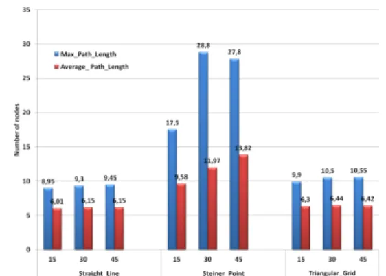
Fig. 5: Total and additional nodes deployed. 3) Path Length to the Sink: Simulation results de-picted in Figure 7, show that the Steiner-Point-based algorithm always provides paths longer than the Straight-Line and Triangular-Grid based algorithms, both in terms of maximum and average path lengths. This is due to the principle of the Steiner-Point algorithm that connects PoIs together. In other words the connectivity of each PoI with the sink is a consequence and not the goal of this algorithm. The main goal being to reduce the
Fig. 6: Total and shared nodes deployed.
number of nodes deployed. However, the Triangular-Grid based algorithm provides results very close to those given by the Straight-Line algorithm, which gives the shortest routes.
Fig. 7: Maximum and average path length to the sink. 4) Computation of the RNP index: Table I shows that the RNP index strongly increases with the number of PoIs for the straight line solution. Its increase is less strong with the Steiner point solution, whereas it is moderate for the triangular grid based solution. In all configurations tested, the triangular grid based solution provides the smallest RNP index. For instance, for 45 PoIs it is 2.8 times less than the straight line.
TABLE I: RNP index for RNP solutions
RNP index
Number Straight-Line Steiner point Triangular grid of nodes based based based
15 675.27 689.5 452.43 30 1439.64 1440 680.92 45 2193.34 1515.1 784.39
V. FAULT-TOLERANTRNP
Assuming that link and/or node failures may occur, we now show how to improve the robustness of the three algorithms described in Section IV. To cope with node and/or link failures, an additional path is built from each PoI to the sink. For any PoI and for any
algorithm considered, the first path to the sink obtained by the algorithm is called the primary path, whereas the others, obtained as explained in this section, are called secondary paths.
A. The Straight-Line Algorithm
a Straight-Line. b Steiner-Point.
Fig. 8: 2-connectivity.
The robustness of the Straight-Line algorithm is en-sured by providing k-connectivity. This algorithm repli-cates each shortest path k − 1 times. Each PoI appears to be at the end of a petal, whose other end is the sink, as depicted in Figure 8a, where 2-connectivity is provided. This algorithm remains very simple but no relay node is shared by the PoIs to reach the sink.
Furthermore, we observe a high concentration of nodes around the sink when the number of PoIs in-creases. This may induce high interference.
B. The Steiner-Point-Based Algorithm
Since in the basic version presented in Section IV, no redundancy is provided, there is no robustness: the failure of a link or node prevents data from at least one PoI reaching the sink. To achieve 2-connectivity, the straight line path from each PoI to the sink is added (see Figure 8b). Hence, there are no additional shared nodes compared with the basic version with only one path per PoI.
C. The Triangular-Grid-Based Algorithm
This solution is made robust by adding one node-disjoint shortest path for each PoI to the sink. This new path shares no nodes with the primary path of the PoI in question, as depicted in Figure 9a. However it may share nodes or links with the primary or secondary path of another PoI, thus reducing the total number of nodes deployed. Figure 9b depicts shared nodes with black circle: at least two paths originating from different PoIs use a shared node to reach the sink. In the triangular lattice of the optimal deployment, each non-border node has 6 neighbor nodes. Consequently, we can obtain any k-connectivity with k ≤ 6. If a higher connectivity is required, another grid structure must be used.
D. Performance Evaluation
These three solutions being enhanced to achieve 2-connectivity, we now compare their performances for various configurations. In addition to the metrics given in Section IV-D1, we add a new metric: the node degree. The RNP index is modified to take into account fault-tolerance. By definition, a fault-tolerant relay node
a Two paths. b Shared nodes.
Fig. 9: 2-connectivity with the Triangular-Grid. placement has an
FT-RNP index = Nr·maxi∈[1,n]Lp(i)·maxi∈[1,n]Ls(i).
1) Number of Sensor Nodes Needed: With regard to the total number of relay nodes deployed, simulation results show that the Triangular-Grid-based algorithm strongly minimizes the total number of relay nodes deployed, as illustrated in Figure 10. For instance, for 45 PoIs, the Triangular-Grid-based algorithm requires a number of additional nodes that is more than 4.25 times smaller than the Straight-Line and 2.6 times smaller than Steiner-Point based algorithm, thus considerably reduc-ing the deployment cost. The number of additional nodes used by the Triangular-Grid-based algorithm increases much smaller than the number of PoIs.
Fig. 10: Total and additional nodes for 2-connectivity.
Fig. 11: Total and shared nodes for 2-connectivity. Simulation results depicted in Figure 11 show that for both the Steiner-Point and the Triangular-Grid based algorithms, the number of shared nodes increases with the number of PoIs. Moreover, with the
Triangular-Grid based algorithm, the deployment around the sink becomes very close to the optimal one defined in [2].
2) Path Length to the Sink: Figure 12 shows that for each algorithm considered, the maximum path length is identical when maintaining one path or two-paths with either the Steiner-Point or the Straight-Line algorithm. For the Triangular-Grid algorithm, the secondary path has a length that is either equal to that of the primary path or greater by one hop. To reduce the data gathering delays in a WSN deployed according to the Steiner-Point algorithm, we recommend exchanging the role of primary and secondary paths by using the Straight-Line path as the primary path.
Fig. 12: Maximum and average path length to the sink for 1 and 2-connectivity.
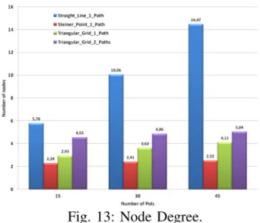
3) Node Degree: In the optimal deployment based on a triangular lattice, each non-border node has exactly 6 neighbor nodes. As a consequence, the degree of any node is upper bounded by 6 for any number of paths k ≤ 6. Simulation results depicted in Figure 13 show that for one path, the average node degree remains in the interval [2, 4] for all the numbers of PoIs tested, whereas for two paths, it remains in the interval [4, 6]. However, with the Straight-Line algorithm, the node degree strongly increases with the number of PoIs, even for a single path. This is due to the very high density of nodes close to the sink and the non-sharing of nodes between the paths. Furthermore, the Steiner-Point algorithm provides the smallest average node degree, because paths are not built toward the sink but between PoIs and relay nodes. More precisely, the sink is considered as a PoI and not as the target destination of any path originating at a PoI. For this reason, with the Steiner-Point algorithm, there is no concentration of nodes around the sink, unlike with the Straight-Line and the Triangular-Grid algorithms as depicted in Figures 3, 1 and 4 respectively.
4) Computation of the FT-RNP index: Table II shows that the triangular grid based solution provides the small-est FT-RNP index in fault-tolerant RNP. This is due to
Fig. 13: Node Degree.
the sharing of relay nodes and the minimized length of both primary and secondary paths.
TABLE II: FT-RNP index for fault-tolerant RNP solu-tions.
FT-RNP index
Number Straight-Line Steiner point Opt deployment 15 12087.46 17988.38 7964.12 30 26777.30 54853.63 11427.41 45 41454.22 75292 12143.10
VI. CONSTRAINED FAULT-TOLERANTRNP In the previous sections, the PoIs and the sink are located in an area that does not contain any obstacles. However, in some applications, this assumption should be relaxed since obstacles may exist. In this section, we focus on ensuring k-connectivity between PoIs and the sink in an environment where obstacles are present. A. The Straight-Line Algorithm
The Straight-Line algorithm that provides the mini-mum number of relay nodes cannot be applied to ensure network connectivity in the presence of obstacles since obstacles may exist on the straight line between the PoI and the sink. However, this solution can be enhanced to cope with obstacles. To keep the characteristic of this method, the relay nodes are deployed along a straight line between the PoI and the sink. The presence of an obstacle on this line is analog to the problem of void handling in geographic routing [10]. One possible solution could be to follow the left-hand rule to bypass the obstacle. However, this solution is not optimal in terms of path length and the number of additional nodes deployed.
B. The Steiner-Point based Algorithm
The Steiner-Point based algorithm cannot cope with the presence of obstacles. Since the computation of the Steiner Point position depends neither on the shape of the area nor on the presence of obstacles, the Steiner Point position could be inside an obstacle. If this position is moved, the mathematical property is lost. Therefore, we do not consider any enhancement of this solution to cope with obstacles.
C. The Triangular-Grid based algorithm
When there is no obstacle in the area considered, the virtual grid of the optimal deployment ensures full area coverage and network connectivity. In this case, at least one path to the sink can be ensured. On the other hand, in the presence of obstacles, not only coverage holes may occur but also isolated PoIs may exist. In fact, when we apply the optimal deployment in an area containing obstacles, nodes that belong to the virtual grid and whose location is inside obstacles are removed, which may result in coverage holes occurring around obstacles. Depending on the PoI position and the sink position, these coverage holes may cause isolated PoIs, particularly if the PoI is surrounded by obstacles.
In a previous study [11], we proposed a solution based on the optimal deployment to ensure full area coverage and network connectivity in the presence of opaque obstacles. We healed coverage holes caused by obstacles by deploying additional nodes in these coverage holes. This final deployment which can cope with obstacles is used as our new virtual grid. Using this virtual grid and the principle of the Triangular-Grid based algorithm, network connectivity can be ensured between each PoI and the sink, as depicted in Figure 14. If now we want to
Fig. 14: Connectivity between each PoI and the sink in the presence of obstacles.
support k-connectivity in the presence of obstacles, we may obtain a network like that depicted in Figure 15 for 2-connectivity. There are two paths with disjoint nodes to connect each PoI to the sink. Hence, the failure of nodes on a single path does not disconnect a PoI. However, we observe two problems:
− bypassing the obstacle leads to a secondary path that is much longer than the primary path (see, for instance, PoI 5 at the bottom right in Figure 15).
− there is a gap between the primary and the secondary paths preventing any node on the primary path from communicating with a node on the secondary path. In Figure 15 we can see a relay node on the primary path of PoI 4 that has no neighbor on the secondary path due to the gap between the two paths.
For each relay node on the secondary path we need to have at least one neighbor on the primary path. As a consequence, any node on the primary path can bypass its successor using a node on the secondary path. To cope with the gap problem, the secondary path should
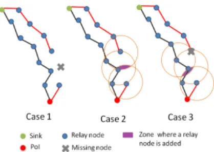
be built using the neighbors of all relay nodes on the primary path instead of all the deployed nodes. Due to the presence of obstacles, some neighbors of the virtual grid may not exist or may not be able to communicate with each other. That is why we propose the rule depicted in Figure 16 where a relay node is added to build the secondary path. The location of this node is critical. First, it should communicate with its downstream neighbor on the secondary path. Second, it should communicate with a relay node of the primary path. Finally, it should communicate with:
• either its upstream neighbor on the secondary path if one exists as depicted in Figure 16 case 2,
• or the upstream neighbor of the relay node in the primary path as illustrated in Figure 16 case 3. Figure 17 shows the final deployment of relay nodes after applying this rule. We can observe that for all the PoIs, any node on the primary path can communicate with a node on the secondary path. Also, we can see the relay node added in pink on the secondary path of PoI 5 which solves two problems: bypassing the obstacle and overcoming the gap between the two paths.
Fig. 15: 2-Connectivity between each PoI and the sink in the presence of obstacles with problems.
Fig. 16: Rule to cope with missing relay nodes when obstacles exist.
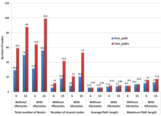
D. Performance Evaluation
In this section, we evaluate the impact of the presence of obstacles in the area depicted in Figure 14, using two configurations: 6 PoIs and 15 PoIs. Results are averaged over several simulations for each configuration (6 and 15 PoIs). The performance evaluation metrics are the total number of relay nodes deployed, the number of shared nodes, the average path length, the maximum path length and the RNP index. In Figure 18, the total number of relay nodes deployed when two paths are needed is
Fig. 17: 2-Connectivity between each PoI and the sink in the presence of obstacles.
less than twice the total number of relay nodes when one path is needed. This is true both with and without obstacles, and is due to the high number of nodes that are shared between paths from different PoIs. For instance, this number reaches 43% of the total number of nodes deployed for 15 PoIs when obstacles exist and two paths are required. The presence of obstacles tends to increase the number of shared nodes in narrow lanes.
The average path length value in the presence of obstacles is close to the average path length value when obstacles do not exist. This is due to the fact that our solution favors a secondary path which is close to the primary one.
The maximum path length depends on the shape of the obstacles. Although the primary and secondary paths are close, the secondary path may be longer than the primary path. This is due to the number and location of the neighbors of all the relay nodes of the primary path. Table III shows the strong impact of the presence
Fig. 18: Evaluation of the impact of obstacles. of obstacle on the RNP index. In addition, maintaining several paths is much more expensive since paths should bypass obstacles.
VII. CONCLUSION
In this paper, we proposed a new solution, called the Triangular-Grid based algorithm, which provides k-connectivity of each PoI to the sink to achieve robustness against link and node failures. Like the Straight-Line algorithm, the Triangular-Grid algorithm provides short
TABLE III: Comparison of RNP index for constrained and unconstrained FT-RNP solution
RNP index: triangular grid based method Number One path Two paths of nodes Without With Without With
obstacles obstacles obstacles obstacles 6 135,93 183,69 1475,02 3463,68 15 262,99 309 2652,22 5634,36
paths. In addition, it minimizes the total number of de-ployed nodes by sharing nodes between paths originating from different PoIs, like the Steiner-Point algorithm. Hence, the Triangular-Grid algorithm minimizes data gathering delays and improves the reliability of each path linking a PoI to the sink and reduces the energy consumed to collect data from PoIs. By limiting the degree of any node, it reduces interferences. In a real environment, obstacles are likely to be present. In such a situation, the Steiner Point-based solution fails to provide a valid deployment, and the Straight Line-based solution may lead to an expensive deployment in terms of the number of relay nodes. In contrast, our solution is able to cope with obstacles while providing robustness by means of disjoint-node paths.
REFERENCES
[1] I. Khoufi, P. Minet, A. Laouiti, and S. Mahfoudh, “Survey of deployment algorithms in wireless sensor networks: coverage and connectivity issues and challenges,” International Journal of Autonomous and Adaptive Communications Systems, 2014. [2] R. Kershner, “The number of circles covering a set,” American
Journal of Mathematics, pp. 665–671, 1939.
[3] S. Lee and M. Younis, “Optimized relay node placement for con-necting disjoint wireless sensor networks,” Computer Networks, vol. 56, no. 12, pp. 2788–2804, 2012.
[4] F. Senel and M. Younis, “Optimized relay node placement for establishing connectivity in sensor networks,” in Global Com-munications Conference (GLOBECOM), 2012, pp. 512–517. [5] H. M. Almasaeid and A. E. Kamal, “On the minimum
k-connectivity repair in wireless sensor networks,” in IEEE Inter-national Conference on Communications, 2009, pp. 1–5. [6] X. Han, X. Cao, E. L. Lloyd, and C.-C. Shen, “Fault-tolerant
re-lay node placement in heterogeneous wireless sensor networks,” IEEE Transactions on Mobile Computing, 2010.
[7] S. Misra, S. D. Hong, G. Xue, and J. Tang, “Constrained relay node placement in wireless sensor networks to meet connectivity and survivability requirements,” in INFOCOM. The 27th Confer-ence on Computer Communications, 2008.
[8] A. Nazi, M. Raj, M. Di Francesco, P. Ghosh, and S. K. Das, “Deployment of robust wireless sensor networks using gene reg-ulatory networks: An isomorphism-based approach,” Pervasive and Mobile Computing, vol. 13, pp. 246–257, 2014.
[9] S. Mahfoudh, I. Khoufi, P. Minet, and A. Laouiti, “GDVFA: A distributed algorithm based on grid and virtual forces for the redeployment of wsns,” in Wireless Communications and Networking Conference (WCNC), 2014, pp. 3040–3045. [10] D. Chen and P. K. Varshney, “Geographic routing in wireless ad
hoc networks,” in Guide to Wireless Ad Hoc Networks. Springer, 2009, pp. 151–188.
[11] I. Khoufi, P. Minet, A. Laouiti, and E. Livolant, “A simple method for the deployment of wireless sensors to ensure full coverage of an irregular area with obstacles,” in Proceedings of the 17th ACM international conference on Modeling, analysis and simulation of wireless and mobile systems, 2014, pp. 203–210.