HAL Id: hal-02975535
https://hal.archives-ouvertes.fr/hal-02975535
Submitted on 22 Oct 2020HAL is a multi-disciplinary open access archive for the deposit and dissemination of sci-entific research documents, whether they are pub-lished or not. The documents may come from teaching and research institutions in France or abroad, or from public or private research centers.
L’archive ouverte pluridisciplinaire HAL, est destinée au dépôt et à la diffusion de documents scientifiques de niveau recherche, publiés ou non, émanant des établissements d’enseignement et de recherche français ou étrangers, des laboratoires publics ou privés.
Revealing the effect of water vapor pressure on the
kinetics of thermal decomposition of magnesium
hydroxide
Satoki Kodani, Shun Iwasaki, Loïc Favergeon, Nobuyoshi Koga
To cite this version:
Satoki Kodani, Shun Iwasaki, Loïc Favergeon, Nobuyoshi Koga. Revealing the effect of water va-por pressure on the kinetics of thermal decomposition of magnesium hydroxide. Physical Chemistry Chemical Physics, Royal Society of Chemistry, 2020, 22 (24), pp.13637-13649. �10.1039/D0CP00446D�. �hal-02975535�
Revealing the effect of water vapor pressure on the kinetics of
thermal decomposition of magnesium hydroxide
Satoki Kodani,1 Shun Iwasaki,1 Loïc Favergeon,2 and Nobuyoshi Koga1,*
1Chemistry Laboratory, Department of Science Education, Graduate School of Education, Hiroshima University,
1-1-1 Kagamiyama, Higashi-Hiroshima 739-8524, Japan.
2Mines Saint-Etienne, University of Lyon, CNRS, UMR 5307 LGF, Centre SPIN, F-42023 Saint-Etienne, France.
Abstract
This study aims to establish an advanced kinetic theory for the reactions in the solid state and solid–gas system, achieving a universal kinetic description over a range of temperature and partial pressure of reactant or product gas. The thermal decomposition of Mg(OH)2 to MgO was selected as a model
reaction system, and the effect of water vapor pressure p(H2O) on the kinetics was investigated using
humidity controlled thermogravimetry. The reaction rate of the thermal decomposition process at a constant temperature was systematically decreased by increasing the p(H2O), accompanied by the
increase in the sigmoidal feature of mass-loss curves. Under nonisothermal conditions at a given heating rate, mass-loss curves shifted systematically to higher temperatures depending on the p(H2O). The
kinetic behavior at different temperature and p(H2O) conditions were universally analyzed by
introducing an accommodation function (AF) of the form (Pº/p(H2O))a[1–(p(H2O)/Peq(T))b], where Pº
and Peq(T) are the standard and equilibrium pressures, respectively, into the fundamental kinetic
equation. Two kinetic approaches were examined based on the isoconversional kinetic relationship and a physico-geometrical consecutive reaction model. In both the kinetic approaches, universal kinetic descriptions are achieved using the modified kinetic equation with the AF. The kinetic features of the thermal decomposition are revealed by correlating the results from the two universal kinetic approaches. Furthermore, advanced features for the kinetic understanding of thermal decomposition of solids revealed by the universal kinetic descriptions are discussed by comparing the present kinetic results with those reported previously for the thermal decomposition of Ca(OH)2 and Cu(OH)2.
Keywords
Thermal decomposition, Mg(OH)2, universal kinetic description, temperature, water vapor pressure
1. Introduction
The thermal decomposition of a solid is the chemical process initiated by nucleation on the reactant surfaces and subsequently advancing at as-generated reaction interfaces.1-4 Thus, the fundamental
kinetic equation generally comprises terms expressing the temperature dependence of the reaction rate like the Arrhenius-type equation and the change in the reaction rate as the reaction advances. The change in the overall reaction rate as advancing the reaction is caused by variation of the effective area of the reaction interface in the scheme of the linear advancement of the reaction interface controlled by a rate-limiting step.5,6 This behavior is usually expressed by a function of the fractional reaction α, i.e., f(α),
termed the kinetic model function.1-4 In addition to the physico-geometrical feature of the heterogeneous
chemical kinetics in the solid state, the evolution of a gaseous product is another characteristic of the thermal decomposition of solids. When the product gas presented in the reaction atmosphere causes a distinguishable effect on the reaction rate of the thermal decomposition, an accommodation function (AF)7 is needed in the fundamental kinetic equation.5,6,8-11 For the simple thermal decomposition of a
solid: A(s) ⇄ B(s) + C(g), the AF may be a function of partial pressure of the product gas p(C(g)) and the equilibrium pressure of the reaction Peq(T), i.e., a(p(C(g)),Peq(T)). The kinetic equation for the
single-step thermal decomposition of solids considering the p(C(g)) is thus expressed as:9, 10
where dα/dt is the normalized reaction rate. The parameters A, Ea, R, and T are the Arrhenius
preexponential factor, apparent activation energy, gas constant, and absolute temperature, respectively. Ideally, eqn (1) implies that the kinetic behavior of the thermal decomposition can be universally described over a range of temperature and p(C(g)) conditions. If the universal kinetic description based on eqn (1) is achieved, further insight into the kinetics of the thermal decomposition of solids via the functional form of the AF and associated parameters can be gained, in addition to the conventional kinetic description via the so-called kinetic triplet, i.e., Ea, A, and f(α).9,10 The success of the universal
kinetic approach based on eqn (1) depends on the AF. The effect of p(C(g)) on the kinetics of thermal decomposition of solids has been investigated for nearly a century.1,12-39 Various functional forms of AF
were derived through theoretical considerations and correlation analysis of the experimental data, 12-21,40-43 and practically utilized for interpreting the effect of p(C(g)) on the kinetics of thermal decomposition
of solids. However, based on our knowledge, the previously derived and examined AF does not necessary describe universally the kinetics over a range of temperature and p(C(g)) conditions based on eqn (1). Recently, the effect of p(H2O) on the kinetics of thermal decomposition of divalent metal
hydroxides exemplified by: M(OH)2(s) ⇄ MO(s) + H2O(g) were reexamined through theoretical
considerations for finding the possible functional forms of AF.9,10 In the theoretical considerations, the
induction period (IP) and mass-loss process of the thermal decomposition were considered as consecutive processes of various elementary steps, based on the classical theories of surface nucleation and interface reaction, respectively. A series of differential kinetic equations for each reaction process were formulated based on the combined rate-limiting step and steady-state assumptions by selecting an elementary step from the consecutive process and assuming the other elementary steps were at equilibrium. Although various kinetic equations were obtained for each reaction step, these are generalized to eqn (2) with variable exponents (a,b).9,10
(2) where Pº is the standard pressure. The applicability of eqn (1) with the AF in eqn (2) was examined experimentally for the IP and mass-loss process for the thermal decomposition of Ca(OH)2 and
Cu(OH)2.9,10 In both metal hydroxides, all data points of the average reaction rates for the IP recorded
at different constant temperatures and p(H2O) values exhibited statistically significant linear correlations
in the modified Arrhenius plot with the appropriate (a,b) values in the AF. Similarly, the mass-loss processes occurring under different heating and p(H2O) conditions were analyzed by the differential
isoconversional plots at various α values based on eqn (1) with the AF, providing the (a,b) and Ea values
as the kinetic parameters for the universal description. Furthermore, because the mass-loss processes under isothermal conditions exhibited sigmoidal shapes for Ca(OH)2 and Cu(OH)2, the overall thermal
decomposition process was characterized by the physico-geometrical consecutive process comprising the IP–surface reaction (SR)–phase boundary-controlled reaction (PBR).44-47 For each component
reaction step, the rate constants determined for the kinetic curves at different constant temperatures and
p(H2O) values were described by a single Arrhenius-type plot based on eqn (1) with the AF.
Consequently, kinetic parameters containing the exponents (a,b) in the AF and the Arrhenius parameters were determined for individual reaction steps of the IP, SR, and PBR. Comparing the thermal decompositions of Ca(OH)2 and Cu(OH)2,9,10 the magnitude relationships between the kinetic
parameters in each reaction step and the variation trends of each kinetic parameter as the reaction step advances were characteristic for the respective thermal decomposition reactions. Based on previous observations, results of the universal kinetic approaches for the reactions at different temperatures and
p(H2O) values further provide insights into the kinetic understanding of the thermal decomposition of
solids.
Herein, the kinetics of the thermal decomposition of Mg(OH)2 under different heating and p(H2O)
conditions are reported as a third examination of the universal kinetic approaches.
(3) Retardation of the overall reaction rate of the thermal decomposition of Mg(OH)2 by atmospheric water
vapor was experimentally demonstrated by Horlock et al.48 and L’vov et al.49 Many previous reports for
the thermal decomposition 45,48-70 were carefully reviewed and the detailed comparison was described in
of Mg(OH)2 under a stream of dry N2 gas were investigated systematically.71 The reaction involved a
major mass-loss process and a subsequent reaction tail. Because the reaction tail was interpreted as the removal of trapped water molecules from the poorly crystalline solid product, i.e., MgO, accompanied by its crystal growth on further heating,57 the major mass-loss process was subjected to a kinetic study
of the chemical reaction. Several features of a partially overlapping two-step process were identified from the conventional kinetic analysis for the reaction under different reaction temperature profiles, including isothermal, linear nonisothermal, and controlled transformation rate conditions.72, 73 The
multistep reaction features were kinetically characterized by two kinetic calculation procedures: (1) kinetic deconvolution analysis74-76 assuming a pseudo-independent two-step process composed of SR
and subsequent PBR in a single reactant body and (2) multiple nonlinear least squares analysis assuming a consecutive SR–PBR model for assemblages of reactant particles.44-47 Although statistically significant
kinetic results were obtained in both the physico-geometrical modeling procedures, the latter kinetic approach was considered more relevant by comparing the kinetic results and considering the possible physico-geometrical reaction mechanisms.In this study, the thermal decomposition of Mg(OH)2 in the
presence of atmospheric water vapor is investigated in detail through the universal kinetic approaches over a range of temperature and p(H2O) conditions to elucidate the physico-geometrical kinetic features
of the reaction. Furthermore, the significance of the proposed universal kinetic approach for understanding the physico-chemical and physico-geometrical features of the thermal decomposition of solids is discussed by comparing the present results with results reported for the thermal decomposition of Ca(OH)2 and Cu(OH)2.9, 10
2. Experimental
2.1 Sample characterization
The Mg(OH)2 sample used in this study is a chemical reagent (special grade, > 99.5%, Wako, Japan)
identical to that used in our previous study.71 The characteristics of the sample, as revealed by the powder
X-ray diffractometry (XRD), Fourier transform infrared spectroscopy (FT-IR), thermogravimetry (TG)– differential thermal analysis (DTA) coupled with mass spectrometry (MS) of the evolved gas, and morphological characterization using scanning electron microscopic (SEM) observation and the Brunauer–Emmett–Teller (BET) specific surface area (SBET) measurement, were already reported in our
previous study.71 In summary, the sample contained agglomerated particles of approximately 50 μm in
diameter (SBET = 34.1 ± 0.3 m2 g-1), constructed by submicron-sized crystalline particles. The powder
XRD pattern was consistent with the previously reported data for Mg(OH)2, i.e., hexagonal, S.G. = P–
3m1(164), a = 3.1498, b = 3.1498, c = 4.7702, ICDD 01-082-2453.77 However, the FT-IR spectrum displayed an absorption peak at 1420 cm-1, which is attributed to the ν
3 mode of CO32-,78 in addition to
the major absorption peaks of the O–H stretching vibration mode at 3695 cm-1 and the Mg–O vibration
at 447 cm-1 originating from Mg(OH)
2.79-83 Under linearly increasing temperature conditions, the
mass-loss curves for the thermal decomposition of Mg(OH)2 exhibited a gradual mass loss in the reaction tail
until approximately 950 K, after the major mass loss in the temperature range of 520–630 K was ended. Most of the evolved gas during the thermal decomposition was water vapor, but a detectable amount of CO2 was present over the mass-loss temperature range. The FT-IR and TG–MS data indicated possible
contamination by a poorly crystalline zinc carbonate compound like hydrozincite.82, 84
2.2 Thermal behavior in atmospheric water vapor
To investigate the effect of atmospheric p(H2O) on the thermal decomposition of Mg(OH)2, TG–
derivative TG (DTG) measurements were conducted under a stream of wet N2 gas characterized by
different p(H2O) values. A sample of approximately 3.0 mg (3.00 ± 0.05 mg) was weighed into a
platinum crucible (5 mm in diameter and 2 mm in height). The sample was placed in the TG–DTA instrument (TG-8120, Thermoplus 2, Rigaku) and heated to 353 K at β = 5 K min-1 under a stream of
dry N2 gas (approximately 400 cm3 min-1). Then, the inflow gas was switched to a wet N2 gas with a
controlled p(H2O) value, generated in the humidity controller (HUM-1, Rigaku).85 After stabilizing the
measurement conditions by maintaining the sample at 353 K, TG–DTG curves were obtained by heating the sample to 773 K at β = 5 K min-1 under a stream of wet N
2 gas with different controlled p(H2O)
values (0.15 kPa ≤ p(H2O) ≤ 7.55 kPa). Details of the instrumental setup for the TG–DTG measurements
2.3 Kinetic measurements
The effect of p(H2O) on the kinetic behavior of the thermal decomposition of Mg(OH)2 was investigated
at different p(H2O) values of 0.15, 1.06, and 5.39 kPa. The same sampling procedures with as those
described above were also used for the measurements of kinetic data. A series of isothermal mass-loss curves at each p(H2O) were obtained by heating the sample to different programmed temperatures at a
β of 5 K min-1, after stabilizing the measurement system at 353 K under the selected p(H
2O) value for
30 min. Subsequently, the sample was held at the programmed temperature until the mass loss ended. Under each p(H2O) value, a series of mass-loss curves under linear nonisothermal conditions were also
obtained by heating the sample to 773 K at different β values (1 ≤ β ≤ 10 K min-1), after stabilizing the
measurement system as in the isothermal measurements.
3. Results and discussion
3.1 Effect of atmospheric water vapor on the mass-loss curve and kinetic measurements
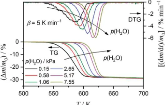
Figure 1 shows TG–DTG curves for the thermal decomposition of the Mg(OH)2 sample at a β of 5 K
min-1 under a stream of wet N2 gas at p(H2O) ranging from 0.15 to 7.55 kPa. All TG curves exhibit a
well-shaped major mass-loss process and subsequent gradual mass-loss that continues at higher temperature. These are similar to those observed for thermal decomposition of the Mg(OH)2 sample
under a stream of dry N2 gas. The observed mass-loss ratios during the major mass-loss process are
independent of the p(H2O) conditions examined in this study, with an average of 28.08 ± 0.2%. The
subsequent gradual mass-loss process is attributed to the release of water molecules trapped in the MgO, triggered by growth of the MgO crystal.57 Thus, complete thermal decomposition was achieved
during the major mass-loss process.71 With increasing p(H
2O) in the reaction atmosphere, the mass-loss
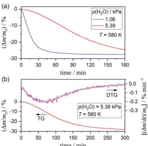
in the TG–DTG curves systematically shift to higher temperatures, accompanied by an increase in the peak top height and decrease in the width of the temperature interval of the DTG peak. This behavior highlights the retardation effect of the atmospheric water vapor on the thermal decomposition of the Mg(OH)2 sample associated with the chemical kinetics. Figure 2 shows the isothermal mass-loss curves
at a constant temperature of 580 K under different p(H2O) conditions. Irrespective of the p(H2O) value,
the mass-loss curves lack evidence of an IP, which differs from the cases of Ca(OH)2 and Cu(OH)2.9,10,22
The total mass-loss under isothermal conditions is practically identical with that for the major mass-loss process under linear nonisothermal conditions. The mass-loss rate is apparently restrained due to the effect of atmospheric water vapor (Figure 2(a)). The isothermal mass-loss curves recorded at a higher
p(H2O) exhibit sigmoidal curves, with the maximum mass-loss rate midway through the overall process
(Figure 2(b)).
Figure 1. TG–DTG curves for thermal decomposition of the Mg(OH)2 sample (m0 = 2.95 ± 0.08 mg) at a β value
of 5 K min-1 under a stream of wet N
2 gas with p(H2O) ranging from 0.15 to 7.55 kPa (flowrate: approximately
Figure 2. Mass-loss curves for thermal decomposition of the Mg(OH)2 sample (m0: approximately 3.0 mg),
recorded at a constant temperature of 580 K under a stream of wet N2 gas with a controlled p(H2O) of 1.06 or 5.39
kPa 190 (flowrate: approximately 400 cm3 min-1): (a) comparison of mass-loss curves recorded at p(H2O) of 1.06
and 5.39 kPa and (b) overall shape of the mass-loss curve and its derivative, recorded at p(H2O) of 5.39 kPa.
The mass-loss data associated with p(H2O) values of 0.15, 1.06, and 5.39 kPa were subjected to the
kinetic calculations, because the curves under these conditions exhibit characteristic mass-loss behaviors in a series of mass-loss curves recorded under different p(H2O) conditions. Mass-loss curves for the
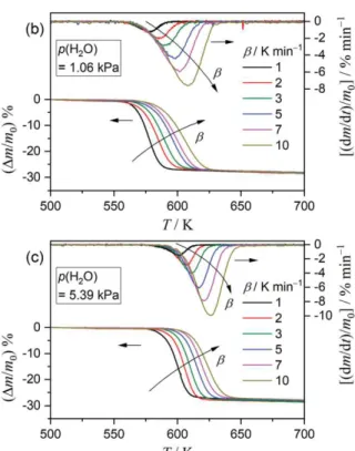
thermal decomposition of the Mg(OH)2 sample at different β values, recorded under a stream of wet N2
gas at three p(H2O) values, are compared in Figure 3. For each series, the mass-loss curves
systematically shift to higher temperatures with increasing β values, exhibiting a typical behavior for the kinetic process. The temperature region where the series of mass-loss curves appeared also shift to higher temperatures with increasing p(H2O). The major mass-loss process observed before the reaction
tail is then subjected to kinetic calculations. The mass-loss curves were transformed to the kinetic curves by normalizing the mass-loss value at any time (Δm(t)) into a fractional reaction (α) referenced to the total mass-loss (Δmtotal) observed during the major mass-loss process.
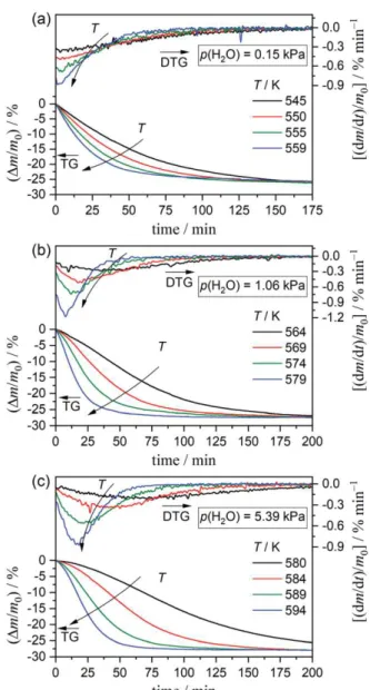
(4) Figure 4 shows three series of mass-loss curves of the thermal decomposition of the Mg(OH)2 samples
at different constant temperatures, recorded at different p(H2O) values of 0.15, 1.06, and 5.39 kPa. In
each series of isothermal mass-loss curves, the total reaction time decreases systematically with increasing reaction temperature. To record the total mass-loss process within an adequate time, the measurement temperature was increased with increasing p(H2O), highlighting a retardation effect due
to atmospheric water vapor. A sigmoidal shape of the mass-loss curves is typically observed for isothermal mass-loss curves obtained at higher p(H2O) conditions and lower temperatures.
Because the Δmtotal values observed under isothermal conditions correspond to those from the major
mass-loss process under linear nonisothermal conditions, the isothermal mass-loss curves were converted to the kinetic curves referenced to the Δmtotal values for the overall process according to eqn
Figure 3. TG–DTG curves for thermal decomposition of the Mg(OH)2 sample under a stream of wet N2 gas with
different controlled p(H2O) values recorded at β values of 1 ≤ β/K min-1 ≤ 10: (a) p(H2O) = 0.15 kPa (m0 = 2.95 ±
Figure 4. Isothermal mass-loss curves for thermal decomposition of the Mg(OH)2 sample under a stream of wet
N2 gas with different controlled p(H2O) values recorded at different constant temperatures: (a) p(H2O) = 0.15 kPa;
545 ≤ T/K ≤ 559 (m0 = 2.98 ± 0.05 mg), (b) p(H2O) = 1.06 kPa; 564 ≤ T/K ≤ 579 (m0 = 3.06 ± 0.10 mg), and (c)
p(H2O) = 5.39 kPa; 580 ≤ T/K ≤ 594 (m0 = 3.07 ± 0.14 mg).
3.2 Formal kinetic analysis without considering the effect of water vapor pressure
As a preliminary approach for the kinetic analysis, the conventional isoconversional method was applied by ignoring the effect of p(H2O) on the reaction, i.e., by applying a(p(H2O),Peq(T))=1 in eqn (1).
Considering logarithms on both sides of eqn (1) with a(p(H2O),Peq(T))=1, the equation for the
conventional Friedman plot86 is obtained:
(5) By plotting ln(dα/dt) against T-1 for the data points at a selected α extracted from the series of kinetic
curves recorded under different temperature conditions, the Ea is obtained from the slope. Figure 5
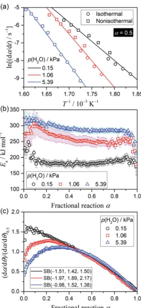
summarizes the results of the kinetic calculations based on eqn (5). Irrespective of the selected α value, the Friedman plots show different linear correlations for the kinetic curves derived under different
p(H2O) conditions, as exemplified by the plots at α = 0.5 (Figure 5(a)), where the slope systematically
increases with increasing p(H2O). Thus, the higher Ea value was evaluated for the reaction with higher
p(H2O) (Figure 5(b)). The apparent Ea decreases during the initial part of the reaction and subsequently
maintains an almost constant value. The average Ea values for 0.1 ≤ α ≤ 0.9 in each reaction under
Figure 5. The results of the formal kinetic analysis for the thermal decomposition of the Mg(OH)2 sample,
performed by ignoring the effect of atmospheric p(H2O): (a) conventional Friedman plots at α = 0.5, (b) Ea values
at various α, and (c) experimental master plot of (dα/dθ)/(dα/dθ)0.5 versus α.
Table 1. Apparent kinetic parameters for the thermal decomposition of the Mg(OH)2 sample at different p(H2O)
values, determined without considering the effect of atmospheric p(H2O).
By assuming a constant Ea during the reaction, changes in the kinetic behavior as the reaction advances
were simulated using an experimental master plot, created by calculating the hypothetical reaction rate (dα/dθ) at infinite temperature at each α value:87-92
(6) with
where θ is Ozawa’s generalized time implying the hypothetical reaction time at infinite temperature in the Arrhenius equation scheme.93,94 The shape of the experimental master plot systematically changes
with the p(H2O) value (Figure 5(c)), with higher contribution of the initial acceleration period for the
for each reaction under various p(H2O) values was fitted using the empirical f(α) known as the Šesták– Berggren model, SB(m, n, p).7, 95, 96
(7) The A value and the kinetic exponents in SB(m, n, p) optimized through fitting are also presented in Table 1.
3.3 Formal kinetic analysis with considering the effect of water vapor pressure
When the effect of p(H2O) on the kinetics of the thermal decomposition is considered by introducing
a((p(H2O)),Peq(T)), the Friedman plot is modified according to eqn (8).9, 10
(8) The most widely accepted AF accounting for the effect of the partial pressure of the product gas p(gas) on the thermal decomposition of solids in general is expressed by:11-14, 18
(9) This simple form of the AF was derived by different researchers on different experimental and theoretical bases. However, the introduction of the AF in eqn (9) into the kinetic equation in eqn (8) failed to significantly improve the Friedman-type plots for the reaction at different p(H2O) values (see
Figure S3 in the ESI). The Ea averaged over 0.1 ≤ α ≤ 0.9 increases systematically with increasing
p(H2O) (Table S1). Therefore, the conventional AF in eqn (9) does not realize the desired universal
kinetic description over a range of temperature and p(H2O) conditions. This was also observed for the
thermal decompositions of Ca(OH)2 and Cu(OH)2 in our previous studies.9,10 In Figure S4, the
experimentally applied p(H2O) values are compared with the Peq(T) values calculated using a
thermodynamic database (MALT2, Kagaku Gijutsu-Sha).97,98 A critical reason for the inconsistent
results is that the p(H2O) values applied to the thermoanalytical measurements are significantly smaller
than the Peq values within the temperature region of the thermal decomposition and the actual reaction
temperature region is much higher than the equilibrium temperature at the applied p(H2O) values.9,10
Therefore, results from eqn (9) are approximately unity for all data points. Thus, the analytical form of the AF in eqn (2) is introduced into eqn (8) for a universal kinetic approach to the reactions over a range of temperature and p(H2O) conditions. When examining the modified Friedman plot, the exponents (a,b)
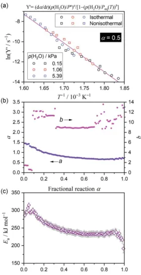
in eqn (2) were optimized at each α value to obtain the best linearity. Figure 6 summarizes the results of the modified Friedman plot using the AF in eqn (2). All data points at a selected α recorded under different temperature and p(H2O) conditions are on a single straight line (Figure 6(a)), confirming a
universal kinetic description. The statistically significant linearity of the modified Friedman plots using the AF in eqn (2) are observed irrespective of the α value (Figure S5). The respective exponents (a,b) in the AF of eqn (2), optimized when examining the modified Friedman plot, exhibit different trends as the overall reaction advances (Figure 6(b)). The exponent b above 8 during the main part of the reaction, followed by much lower b values (0.5–1.5) in the initial part of the reaction (α ≤ 0.08). Since the p(H2O)
value is much lower than the Peq(T) value for all data points, the second part of the AF in eqn (2), i.e.,
1–(p(H2O)/Peq(T))b, is approximated to unity in the main part of the reaction with such a large b value.
Thus, the universal description of the kinetic behavior over a range of temperature and p(H2O)
conditions is achieved by the first part of the AF in eqn (2), i.e., (Pº/p(H2O))a. The exponent a decreases
gradually from approximately 1.5 to 0.7 during the first-half of the reaction (0.01 ≤ α ≤ 0.60) and subsequently converges to an approximately constant value of 0.68 ± 0.02 (0.60 ≤ α ≤ 0.95). The Ea
values calculated from the slope of the modified Friedman plot at different α values also gradually decrease from approximately 300 kJ mol-1 to 235 kJ mol-1 (0.01 ≤ α ≤ 0.60), and subsequently attain a
constant value of 233.8 ± 2.8 kJ mol-1 (0.60 ≤ α ≤ 0.95) (Figure 6(c)). The E
a variation trend as the
reaction proceeds is perfectly synchronized with that of the a value in the AF, which was also observed for Ca(OH)2.9 The trend is contrary to that observed for the thermal decomposition of the same Mg(OH)2
sample under a stream of dry N2 gas,71 where a lower Ea value was calculated for the initial part of the
Figure 6. Results of the modified Friedman plot with the AF in eqn (2), applied universally to the kinetic curves
derived for the thermal decomposition of the Mg(OH)2 sample under different temperature and p(H2O) conditions:
(a) the modified Friedman plot at α of 0.5, (b) the optimized exponents (a,b) in the AF of eqn (2) at various α values, and (c) the Ea values at various α values.
3.4 Universal kinetic modeling of the physico-geometrical consecutive process over a range of temperature and p(H2O) conditions
The apparent variation of the Ea value accompanied by that of the exponent a in the AF of eqn (2) as the
reaction advances indicate a change in the reaction mechanism during the reaction. In our previous study for the thermal decomposition of the same Mg(OH)2 sample under a stream of dry N2 gas,71, a
consecutive SR– PBR(n) model with an interface shrinkage dimension of 2 or 3 was selected as a possible kinetic model for describing the overall kinetics of the reaction. The reaction, as described by the SR–PBR(n) model, exhibits a sigmoidal mass-loss curve under isothermal conditions, with this also observed for the present study in the presence of atmospheric water vapor (Figures 2 and 4). In addition, the sigmoidal trend appears more clearly for reactions at higher p(H2O) conditions. In the kinetic
modeling scheme based on the SR–PBR(n) model, the kinetic behavior of the SR and PBR can be separately characterized; thus, a possibility to examine the effect of p(H2O) on each physico-geometrical
reaction step exists.9, 10 The kinetic calculation based on the SR–PBR(n) model was performed using the
differential kinetic equations derived by assuming a first-order rate law for the SR process and an interface shrinkage dimension n (Table S2).46 Each experimental kinetic curve recorded at specified
temperature and p(H2O) conditions was fitted by the differential kinetic equation, enabling optimization
of the rate constants for the SR (kSR) and PBR(n) (kPBR(n)) by the nonlinear least squares analysis with
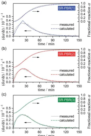
the Levenberg–Marquardt algorithm. The detailed calculation procedures are described in Section S4 in the ESI. Figure 7 shows typical fitting results for different assumed n values. Irrespective of the temperature and p(H2O) conditions, the SR–PBR(3) model represents the most statistically significant
fit to the experimental kinetic curve. Each elementary particle of Mg(OH)2 is usually a hexagonal thin
plate, and the 2D shrinkage of the reaction interface in each particle, formed initially at the edge surfaces, is consistent with previous studies.51,53,55-57 However, the Mg(OH)
2 sample in the present study is
characterized as agglomerates of crystalline particles with diameters of approximately 50 μm.71 The
apparent best fit using the SR–PBR(3) model likely indicates the overall kinetics of thermal decomposition of the agglomerates. The optimized kSR and kPBR(3) values at different temperature and
p(H2O) conditions are presented in Table S3.
Figure 7. Typical fitting results for the experimental kinetic curve (T = 589 K; p(H2O) = 5.39 kPa) by the SR–
PBR(n) model: (a) n = 1, (b) n = 2, and (c) n = 3.
The temperature dependences of the rate constants for the individual reaction steps were initially examined using the conventional Arrhenius plot without considering the effect of p(H2O). Figure S6
shows that the rate constants determined at different p(H2O) conditions exhibit varying linear
correlations in the conventional Arrhenius plot irrespective of the reaction step. In addition, the calculated Arrhenius parameters show no indication of systematic dependence on p(H2O) (Table S4).
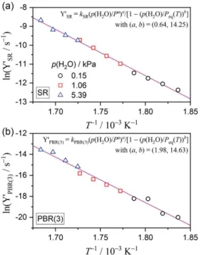
As for the modified Friedman plot using the AF in eqn (9), the situation remained unchanged despite introduction of the conventional AF. Thus, the Arrhenius plot was modified by introducing the AF in eqn (2). Figure 8 shows the modified Arrhenius plots using the AF in eqn (2) for each reaction step, with the exponents (a, b) in the AF optimized to obtain the best linearity in each Arrhenius plot. In each reaction step, all rate constants determined for the reaction at different temperature and
p(H2O) values are described by a single Arrhenius plot. The Arrhenius parameters determined
universally for the reactions under different temperature and p(H2O) values are presented in Table 2. In
both the reaction steps, the exponent b in the AF exhibits a large value. Thus, the second part of the AF, i.e., (1–(p(H2O)/Peq(T))b), is approximated to unity, and the effect of p(H2O) is accommodated in the
universal kinetic expression, owing to the first part of the AF in eqn (2), i.e., (Pº/p(H2O))a. The a values
for the SR and PBR(3) steps are significantly different with a magnitude relationship, i.e., a(SR) <
a(PBR(3)), indicating different effects of p(H2O) on various reaction steps. Similar magnitude
relationships are evident for the Ea and A values, i.e., Ea(SR) < Ea(PBR(3)) and A(SR) < A(PBR(3)).
interpreted considering the kinetic compensation effect (KCE).99-106 Thus, the relationships of the actual
reaction rates should be interpreted by considering the KCE.
Figure 8. Modified Arrhenius plots with the AF in eqn (2) for the reaction steps of (a) SR and (b) PBR(3).
Table 2. Exponents (a,b) of the AF in eqn (2) and the Arrhenius parameters determined by the modified Arrhenius
plots for the individual reaction steps
3.5 Interpretation of the apparent kinetic results
Both kinetic approaches examined by introducing the AF in eqn (2), i.e., the kinetic analysis based on the modified isoconversional analysis and that based on the physico-geometrical consecutive SR– PBR(n) model, achieved universal kinetic description over a range of temperature and p(H2O)
conditions, with linear kinetic plots (Figures 6(a) and 8). However, the apparent kinetic results from the two approaches are characterized by significant discrepancies. The effect of p(H2O) was accommodated
by the first part of the AF with the exponent a for both. However, opposite trends occur for the a values as the reaction advances for the two approaches. The isoconversional kinetic approach shows gradual decrease in the a values during the first-half of the overall reaction (Figure 6(b)). Contrarily, in the kinetic approach based on the SR–PBR(3) model, the primary SR yield a lower a value compared with that for the subsequent PBR(3). The opposite trend is also observed for the apparent Ea values.
The Ea values determined by the modified Friedman plots gradually decrease, synchronizing with the
variation of a values in one approach (Figure 6(c)), whereas, the lower Ea value was obtained for the SR
in comparison with that for the PBR(3) in the other approach (Table 2). The kinetic results obtained by the modified isoconversional kinetic approach can be further validated by reexamining the theoretical basis of the kinetic calculation method.5,76,86,93 In any isoconversional kinetic approach, an invariant
physico-geometrical reaction mechanism covering the reaction conditions is a prerequisite. For the thermal decomposition of the Mg(OH)2 sample in the presence of atmospheric water vapor, the apparent
Ea values, evaluated for the reactions under different heating conditions at a selected p(H2O) without
considering its effect, exhibits systematic variation as the reaction advances (Figure 5(b)). This suggests that the mechanistic feature of the reaction varies with heating conditions even at constant p(H2O).
sigmoidal shapes as the p(H2O) value increases (Figure 4), as prominently illustrated by changes in the
experimental master plots for reactions at different p(H2O) conditions (Figure 5(c)). This observation
indicates that 395 the mechanistic feature of the reaction also changes with the p(H2O) value. Strictly,
the expected variations of the physico-geometrical reaction mechanism with temperature and p(H2O) do
not satisfy the prerequisite of the isoconversional kinetic approach, producing the apparent variation of
Ea as the reaction advances. In the kinetic equation of eqn (1), the AF in eqn (2) is introduced as a
preexponential term. The AF acts as the correction term for the A value, universally expressing the reaction rate at different p(H2O) values, with the functional form of f(α) invariant over the range of the
reaction conditions applied to the kinetic calculation. When the mechanistic feature of the reaction varies with p(H2O) value, the variations in the f(α) value for the data points recorded at different p(H2O)
conditions are also accommodated by the AF, providing the best linearity for the isoconversional kinetic plot by optimizing the exponents (a, b). Accordingly, the exponents (a, b) determined by the modified Friedman plots at the various α values are the apparent values, with the mechanistic features changing depending on the p(H2O) value, as well as the heating conditions. The apparent (a,b) values directly
influence the intercept of the modified Friedman plot, i.e., ln[Af(α)], further inducing a compensative change in the slope of the plot, and thus, the apparent Ea value like the KCE.99-106 The correlation
between the exponents (a,b) and the Ea value determined by the modified Friedman plot is evident for
the synchronized variations between a and Ea in Figure 6(b) and (c). In cases like the thermal decomposition of the Mg(OH)2 samples in the presence of atmospheric water vapor, the exponents (a,b)
determined through the modified Friedman plot cannot be directly correlated to the effect of p(H2O).
The variations of the mechanistic feature of the reaction is explained by changes in the kinetic contributions of the SR and PBR to the overall reaction with varying p(H2O). In the kinetic approach
based on the SR–PBR model, the changes in the kinetic contributions are considered during kinetic fitting of the isothermal mass-loss curves, and the rate constants for SR and PBR are separately optimized at each set of temperature and p(H2O) conditions. Thus, the variation of the mechanistic
feature does not affect the optimized rate constants and the modified Arrhenius plots for each reaction step. For the thermal decomposition of the same Mg(OH)2 sample under a stream of dry N2 gas, previous
study indicates that the apparent Arrhenius parameters (Ea/kJ mol-1, ln(A/s-1)) for the SR and PBR(3)
determined using the conventional Arrhenius plot were (135.3 ± 2.6, 22.2 ± 0.6)SR and (247.2 ± 7.3, 49.1
± 1.6)PBR(3), respectively.71 The magnitude relationships of these sets of Arrhenius parameters for the SR
and PBR(3) are identical to those determined for the reaction under the presence of atmospheric water vapor in this study. The correspondence between the kinetic results obtained for the reaction under a stream of dry N2 gas and under the presence of the atmospheric water vapor is interpreted as evidence
for evaluating the kinetic description based on the SR–PBR model. However, the values determined for the reaction over a range of temperature and p(H2O) conditions are higher than those in a dry N2
atmosphere. Although the difference for the Arrhenius parameters in each reaction step between the reactions under different atmospheric conditions are superficially correlated via the KCE,99-106 it must
be acknowledged that these Arrhenius parameters were determined on different bases of kinetic modeling. Alternatively, the kinetic parameters determined through the modified Arrhenius plot with the AF in eqn (2) represent these physico-chemical meaning only when the exponents (a,b) are accompanied. Considering the mutual dependence of the kinetic parameters, the introduction of the AF influences the apparent A value, and interacts with the apparent Ea value in the KCE scheme.
3.6 Comparison with the reactions of the other metal hydroxides
In comparison with other metal hydroxides studied previously,9,10 the thermal decomposition of the
Mg(OH)2 sample in the presence of atmospheric water vapor exhibits specific kinetic features. A
distinguishable difference is the lack of an IP before the mass-loss process begins. Significant IPs were observed for thermal decomposition of Cu(OH)2 irrespective of the presence or absence of atmospheric
water vapor and for Ca(OH)2 in the presence of water vapor. The variation features of the mass-loss
curves with increasing p(H2O) also differ for the thermal decompositions of these metal hydroxides. The
thermal decompositions of Mg(OH)2 and Cu(OH)2 display the sigmoidal mass-loss curves under
isothermal conditions irrespective of the presence or absence of atmospheric water vapor; whereas, the behavior was only observed in the presence of water vapor for Ca(OH)2. When the conventional
isoconversional method is applied without considering the effect of the atmospheric water vapor, the apparent Ea values increase with increasing p(H2O) value for all thermal decompositions. The Ea values
for the thermal decompositions of Mg(OH)2 and Cu(OH)2 at each p(H2O) value are approximately
constant during the main part of the reaction (Figure 5(b) and Table 1); while, systematic variation of
Ea value as the reaction advances is evident for Ca(OH)2. The difference between the thermal
decompositions of Mg(OH)2 and Cu(OH)2 emerges in the experimental master plots of (dα/dθ)/(dα/dθ)0.5
versus α at different p(H2O) values drawn using the apparent Ea values obtained by the conventional
isoconversional method (Figure 5(c)). Although the experimental master plots for the thermal decomposition of Cu(OH)2 are practically similar irrespective of the p(H2O) value, those for the thermal
decomposition of Mg(OH)2 display systematic changes with increasing p(H2O), with the variation
indicating the increasing kinetic contribution of the SR on the overall kinetics. The introduction of the AF in eqn (2) into the Friedman plot enabled universal kinetic analyses for the mass-loss process of the thermal decompositions of each metal hydroxide over a range of temperature and p(H2O) conditions.
The optimized sets of exponents (a,b) in the AF and variations as the reaction advances seen in the results characterize features of the effect of p(H2O) on kinetics of the mass-loss process. The second
part of the AF in eqn (2) involving the relative magnitude of p(H2O) with reference to Peq(T) and
exponent b, evaluating the distance of the actual reaction from the equilibrium condition for temperature and p(H2O). When the p(H2O) value is significantly lower than Peq(T) value, the contribution of the
second part of the AF to the universal kinetic description under different p(H2O) conditions is limited.
This is further evidenced when the empirically optimized b value is unexpectedly high. In the universal approach using the modified Friedman plots, such unexpectedly large b value was obtained for the thermal decompositions of Mg(OH)2 and Cu(OH)2, i.e., b > 8. These reactions occur at much lower
p(H2O) value with reference to Peq(T) value in the actual reaction temperature region. Alternatively, the
actual reaction temperature region is much higher than the equilibrium temperature at the applied p(H2O)
value. For the thermal decomposition of Ca(OH)2, b values are almost constant, with an average of 1.28
± 0.07 (0.04 ≤ α ≤ 0.97) obtained from the isoconversional kinetic analysis. Although, even in this case, the contribution of the second part of the AF to achieve the universal kinetic description at different temperature and p(H2O) conditions is limited in comparison with the first part of the AF, the second part
corrects the slope of the Arrhenius-type plots. In all these thermal decompositions, the first part of the AF with the exponent a predominantly influenced the achievement of the universal kinetic description. However, the exponent a, optimized through the modified Friedman plots at various α values, exhibits different variation trends for the reactions. The a values were almost constant, with an average of 0.36 ± 0.03 (0.04 ≤ α ≤ 0.97) characterizing the effect of p(H2O) on the kinetics of thermal decomposition of
Cu(OH)2 based on the isoconversional kinetic relationship. For this process, the Ea was also
approximately constant during the reaction, with an average of 148.1 ± 3.3 kJ mol-1 (0.05 ≤ α ≤ 0.95).
Conversely, the optimized a values change systematically as the reaction proceeds for the thermal decomposition of Mg(OH)2 and Ca(OH)2. This variation is accompanied by changes in the apparent Ea
values with similar variation trend. Two possible reasons account for the synchronized variations in the
a and Ea values as the reaction progresses. The first is the change in the effect of the p(H2O) value as
the reaction proceeds, probably caused by the physicochemical reaction mechanism during the reaction. The second is the change in the mechanistic feature of the overall reaction with the applied p(H2O)
value, as discussed previously for the thermal decomposition of Mg(OH)2. In the latter case, the
preliminary assumption of the isoconversional kinetic approach, i.e., the invariant f(α) among the reactions under the examined conditions, is not fulfilled, producing the apparent values of the exponent
a and Ea. Probably, in some cases, the synchronized variations of a and Ea values also result from the
coupled effects of changes in the physico-geometrical reaction mechanism with α and p(H2O), as well
as heating conditions. Thus, the kinetic results from the modified Friedman plot with the AF in eqn (2) requires careful interpretation for the physicogeometrical reaction mechanism and the applicability of the isoconversional method. For the thermal decompositions of these metal hydroxides in the presence of atmospheric water vapor, the mass-loss processes under isothermal conditions are satisfactory described by the SR–PBR(n) model. With this model, the possible variation of the mechanistic feature of the reactions with reaction temperature and p(H2O) conditions can be treated as changes in the kinetic
contributions of the SR and PBR(n). Application of the modified Arrhenius plot using the AF in eqn (2) to the optimized rate constants for each physico-geometrical reaction step produced the universal kinetic description for each reaction step under different temperature and p(H2O) conditions.
However, the relationship of the resulting kinetic parameters between SR and PBR(n) and those corresponding to the kinetic parameters determined by the modified Friedman plot are different for the
mass-loss processes for the metal hydroxides. For comparison with the present results for the thermal decomposition of Mg(OH)2 (Table 2), previously reported kinetic parameters for the thermal
decompositions of Ca(OH)2 and Cu(OH)2 are presented in Table S5. Regarding the optimized exponents
(a, b) in the AF, the magnitude relationships between (a, b) values in each reaction step are comparable with those determined by the modified Friedman plot for reactions of three metal hydroxides. For the thermal decompositions of Ca(OH)2 and Cu(OH)2, the changes in the a values as the reaction advances
from SR to PBR(n) also follow expected trends from the modified Friedman plot, i.e., a(SR) >
a(PBR(2)) for Ca(OH)2 and a(SR) ≈ a(PBR(1)) for Cu(OH)2. However, the magnitude relationship of
a(SR) < a(PBR(3)) observed for the thermal decomposition of Mg(OH)2 is the opposite expected from
the modified Friedman plot exhibiting systematic decrease in the a value as the reaction proceeds. The same magnitude relationship observed for the a values for SR and PBR(n) in each reaction for the metal hydroxides is observed for the Ea values, i.e., Ea(SR) > Ea(PBR(2)) for Ca(OH)2, Ea(SR) ≈ Ea(PBR(1))
for Cu(OH)2, and Ea(SR) < Ea(PBR(3)) for Mg(OH)2, with that for Mg(OH)2 opposite that expected
from the modified Friedman plot. The A values for SR and PBR(n) also follow the same magnitude relationship in each reaction like the a and Ea values. Thus, the thermal decompositions of those three
metal hydroxides in the presence of atmospheric water vapor are characterized by different magnitude relationships between the exponents (a, b) in the AF of eqn (2) and the variation trends of the kinetic parameters, including the (a, b) values and the Arrhenius parameters, as the reaction advances from SR to PBR. These kinetic parameters reflect the characteristics of the kinetic behaviors changing with the heating and atmospheric conditions. Therefore, patterns and trends of the parameter relationships in each reaction step and between different reaction steps provide indexes for the classification of the kinetic characteristics of thermal decomposition of solids, considering the effects of temperature and partial pressure of the product gas. Further studies on the kinetics of different thermal decomposition reactions using the universal kinetic approaches are necessary for establishing novel theoretical basis for understanding kinetics.
4. Conclusions
Thermal decomposition of Mg(OH)2 occurred at a lower p(H2O) value with reference to the Peq(T) at
the reaction temperature region, which was much higher than the equilibrium temperature at the applied
p(H2O) value. The reaction rate was significantly reduced by atmospheric water vapor, as evidenced by
prolongation of the reaction time at constant temperature and systematic shift of the mass-loss curves recorded at a β to higher temperatures with increasing p(H2O) values. Under isothermal conditions, a
sigmoidal shape of the mass-loss curve was more distinguishable with increasing p(H2O) value and
decreasing reaction temperature. The reaction in this study also showed no IP for temperatures and
p(H2O) values examined. The changes in the kinetic behaviors with heating and atmospheric conditions
were universally demonstrated by introducing the analytical form of the AF in eqn (2) into the fundamental kinetic equation. In the isoconversional kinetic approach, the universal kinetic description was achieved by the modified Friedman plot at each α value through optimizing the exponent (a,b) in the AF, exhibiting statistically significant linear correlations for all data points at a given α recorded at different heating and p(H2O) conditions. The predominant role of the exponent a over b for achieving
the universal kinetic description emerged as a characteristic of the present reaction. However, both the exponent a and Ea values determined through the modified Friedman plot decreased in the first-half of
the reaction as the reaction advanced, followed by approximately constant values in the second-half of the reaction. The overall mass-loss curves recorded under isothermal conditions were adequately described by the physico-geometrical consecutive SR–PBR(3) model, as expected from the sigmoidal shape of the mass-loss curves and the variation of the Ea value determined by the isoconversional method as the reaction advanced. Based on the SR–PBR(3) model, the universal kinetic description over a range of temperature and p(H2O) conditions were achieved for each physico-geometrical reaction step
by the Arrhenius plot modified by introducing the AF in eqn (2). This enabled us to separately evaluate the effect of p(H2O) on the various reaction steps. However, the magnitude relationships of a(SR) <
a(PBR(3)) and Ea(SR) < Ea(PBR(3)) estimated by the modified Arrhenius plots showed trends opposite
the expectations from results of the modified Friedman plots. The discrepancies were interpreted as caused by the change in the mechanistic feature of the reaction with the applied p(H2O) value; thus, the
application of the modified Friedman plots at different p(H2O) values does not fulfil the preliminary
universal kinetic description based on the SR–PBR(n) model for the thermal decompositions of Ca(OH)2
and Cu(OH)2, the three reactions including that of Mg(OH)2 exhibited different magnitude relationships
between the optimized kinetic parameters in each reaction step and different physico-geometrical reaction steps. The patterns and trends of the parameter relationships are used for characterizing the kinetics of the thermal decomposition of solids in the scheme of universal kinetic description at different temperatures and partial pressures of the product gas, based on the physico-geometrical consecutive reaction models.
Conflicts of Interest
There are no conflicts of interest to declare. Corresponding Author
*Tel./fax: +81-82-424-7092. E-mail: nkoga@hiroshima-u.ac.jp
Acknowledgements
The present work was supported by JSPS KAKENHI Grant Numbers 17H00820.
References
1. A.K. Galwey and M.E. Brown, Thermal Decomposition of Ionic Solids, Elsevier, Amsterdam, 1999. 2. A.K. Galwey, Thermochim. Acta, 2000, 355, 181-238.
3. N. Koga and H. Tanaka, Thermochim. Acta, 2002, 388, 41-61.
4. N. Koga, Y. Goshi, M. Yoshikawa and T. Tatsuoka, J. Chem. Educ., 2014, 91, 239-245. 5. N. Koga, J. Therm. Anal. Calorim., 2013, 113, 1527-1541.
6. N. Koga, J. Šesták and P. Simon, in Thermal analysis of Micro, Nano- and Non-Crystalline Materials, eds. J. Šesták and P. Simon, Springer, 2013, ch. Chap. 1, pp. 1-28.
7. J. Šesták, 1990, 36, 1997-2007.
8. S. Vyazovkin, A.K. Burnham, J.M. Criado, L.A. Pérez-Maqueda, C. Popescu and N. Sbirrazzuoli, Thermochim.
Acta, 2011, 520, 1-19.
9. N. Koga, L. Favergeon and S. Kodani, Phys. Chem. Chem. Phys., 2019, 21, 11615-11632. 10. M. Fukuda, L. Favergeon and N. Koga, J. Phys. Chem. C, 2019, 123, 20903-20915. 11. S. Vyazovkin, Int. Rev. Phys. Chem., 2019, 39, 35-66.
12. A.F. Benton and L.C. Drake, J. Am. Chem. Soc., 1934, 56, 255-263. 13. J. Zawadzki and S. Bretsznajder, Trans. Faraday Soc., 1938, 34, 951-959. 14. T.R. Ingraham and P. Marier, Can. J. Chem. Eng., 1963, 41, 170-173. 15. J.M. Criado, F. Gonzalez and M. Gonzalez, J. Therm. Anal., 1982, 24, 59-65. 16. J.M. Criado, M. González and M. Macías, Thermochim. Acta, 1987, 113, 39-47. 17. J.M. Criado, M. González and M. Macías, Thermochim. Acta, 1987, 113, 31-38.
18. J. Criado, M. González, J. Málek and A. Ortega, Thermochim. Acta, 1995, 254, 121-127. 19. J. Khinast, G.F. Krammer, C. Brunner and G. Staudinger, Chem. Eng. Sci., 1996, 51, 623-634. 20. C.K. Clayton and K.J. Whitty, Appl. Energy, 2014, 116, 416-423.
21. J. Yin, X. Kang, C. Qin, B. Feng, A. Veeraragavan and D. Saulov, Fuel Process. Technol., 2014, 125, 125-138.
22. M. Fukuda and N. Koga, J. Phys. Chem. C, 2018, 122, 12869-12879.
23. W. E. Garner, in Chemistry of the Solid State, ed. W. E. Garrner, Butterworths, London, 1955, ch. 8, pp. 213-231.
24. D.A. Young, Decomposition of Solids, Pergamon, Oxford, 1966.
25. F.C. Tompkins, in Treates on Solid State Chemistry, Vol. 4 Reactivity of Solids, ed. N.B. Hannay, Plenum, New-York, 1976, vol. 4, ch. 4, pp. 193-231.
26. M.E. Brown, D. Dollimore and A.K. Galwey, Reactions in the Solid State, Elsevier, Amsterdam, 1980. 27. B. Topley and M.L. Smith, Nature, 1931, 128, 302-302.
28. B. Topley and M.L. Smith, J. Chem. Soc., 1935, 321-324. 29. M. Volmer and G. Seydel, Z. Phys. Chem., 1937, 179A, 153-171.
30. B.V. L'Vov, A.V. Novichikhin and A.O. Dyakov, Thermochim. Acta, 1998, 315, 169-179. 31. N. Koga, J.M. Criado and H. Tanaka, Thermochim. Acta, 1999, 340-341, 387-394. 32. N. Koga, J.M. Criado and H. Tanaka, 2000, 60, 943-954.
33. N. Koga and S. Yamada, Int. J. Chem. Kinet., 2005, 37, 346-354.
34. N. Koga, T. Tatsuoka and Y. Tanaka, J. Therm. Anal. Calorim., 2009, 95, 483-487. 35. S. Yamada and N. Koga, Thermochim. Acta, 2005, 431, 38-43.
36. N. Koga, S. Maruta, T. Kimura and S. Yamada, J. Phys. Chem. A, 2011, 115, 14417-14429. 37. S. Yamada, E. Tsukumo and N. Koga, J. Therm. Anal. Calorim., 2009, 95, 489-493.
38. N. Koga, T. Tatsuoka, Y. Tanaka and S. Yamada, Trans. Mater. Res. Soc. Jpn., 2009, 34, 343-346. 39. M. Nakano, T. Fujiwara and N. Koga, J. Phys. Chem. C, 2016, 120, 8841-8854.
40. T. Liavitskaya and S. Vyazovkin, J. Phys. Chem. C, 2017, 121, 15392-15401.
41. M. Deutsch, F. Birkelbach, C. Knoll, M. Harasek, A. Werner and F. Winter, Thermochim. Acta, 2017, 654, 168-178.
42. E.P. Hyatt, I.B. Cutler and M.E. Wadsworth, J. Am. Ceram. Soc., 1958, 41, 70-74.
43. J.M. Valverde, P.E. Sanchez-Jimenez and L.A. Perez-Maqueda, J. Phys. Chem. C, 2015, 119, 1623-1641. 44. K. L. Mampel, Z. Phys. Chem., Abt. A, 1940, 187, 43-57.
45. H. Yoshioka, K. Amita and G. Hashizume, Netsu Sokutei, 1984, 11, 115-118. 46. H. Ogasawara and N. Koga, J. Phys. Chem. A, 2014, 118, 2401-2412.
47. L. Favergeon, M. Pijolat and M. Soustelle, Thermochim. Acta, 2017, 654, 18-27. 48. R.F. Horlock, P.L. Morgan and P. J. Anderson, Trans. Faraday Soc., 1963, 59, 721-728. 49. B.V. L'Vov, A.V. Novichikhin and A.O. Dyakov, Thermochim. Acta, 1998, 315, 135-143. 50. J.F. Goodman, Proc. R. Soc. London, Ser. A, 1958, 247, 346-352.
51. P.J. Anderson and R.F. Horlock, Trans. Faraday Soc., 1962, 58, 1993-2004.
52. G.W. Brindley, in Progress in Ceramic Science, ed. J.E. Burke, Pergamon Oxford, 1963, vol. 3, ch. 1, pp. 1-56.
53. R.S. Gordon and W.D. Kingery, J. Am. Ceram. Soc., 1966, 49, 654-660.
54. N.H. Brett, K.J.D. MacKenzie and J. H. Sharp, Q. Rev., Chem. Soc., 1970, 24, 185-207. 55. F. Freund, R. Martens and N. Scheikh-ol-Eslami, J. Therm. Anal., 1975, 8, 525-529. 56. M.G. Kim, U. Dahmen and A.W. Searcy, J. Am. Ceram. Soc., 1987, 70, 146-154. 57. H. Naono, Colloids Surf., 1989, 37, 55-70.
58. K.J.D. MacKenzie and R.H. Meinhold, Thermochim. Acta, 1993, 230, 339-343.
59. T. Yoshida, T. Tanaka, H. Yoshida, T. Funabiki, S. Yoshida and T. Murata, J. Phys. Chem., 1995, 99, 10890- 10896.
60. S.J. Gregg and R.I. Razouk, J. Chem. Soc., 1949, S36-S44
61. R.C. Turner, I. Hoffman and D. Chen, Can. J. Chem., 1963, 41, 243-251. 62. R.S. Gordon and W.D. Kingery, J. Am. Ceram. Soc., 1967, 50, 8-14. 63. P.H. Fong and D.T.Y. Chen, Thermochim. Acta, 1977, 18, 273-285. 64. A. Bhatti, D. Dollimore and A. Dyer, Thermochim. Acta, 1984, 78, 55-62. 65. I. Chen, S.K. Hwang and S. Chen, Ind. Eng. Chem. Res., 1989, 28, 738-742. 66. I. Halikia, P. Neou-Syngouna and D. Kolitsa, Thermochim. Acta, 1998, 320, 75-88. 67. L.H. Yue, D.L. Jin, D.Y. Lu and Z.D. Xu, Acta Phys.-Chim. Sin., 2005, 21, 752-757. 68. K. Nahdi, F. Rouquerol and M. Trabelsi Ayadi, Solid State Sci., 2009, 11, 1028-1034. 69. R. Trittschack, B. Grobéty and P. Brodard, Phys. Chem. Miner., 2013, 41, 197-214. 70. C. Liu, T. Liu and D. Wang, J. Therm. Anal. Calorim., 2018, 134, 2339-2347.
71. S. Iwasaki, S. Kodani and N. Koga, J. Phys. Chem. C, 2020., 124, 2458-2471. DOI: 10.1021/acs.jpcc.9b09656. 72. O.T. Toft Sοrensen and J. Rouquerol, Sample Controlled Thermal Analysis, Kluwer, Dordrecht, 2003. 73. J.M. Criado, L.A. Perez-Maqueda and N. Koga, in Thermal Physics and Thermal Analysis, eds. J. Šesták, P. Hubík and J.J. Mareš, Springer Nature, Switzerland, 2017, ch. 2, pp. 11-43.
74. P.E. Sánchez-Jiménez, A. Perejón, J.M. Criado, M.J. Diánez and L.A. Pérez-Maqueda, 2010, 51, 3998-4007. 75. N. Koga, Y. Goshi, S. Yamada and L.A. Pérez-Maqueda, J. Therm. Anal. Calorim., 2013, 111, 1463-1474. 76. N. Koga, in Handbook of Thermal Analysis and Calorimetry, eds. S. Vyazovkin, N. Koga and C. Schick, Elsevier, Amsterdam, 2nd edn., 2018, vol. 6, ch. 6, pp. 213-251.
77. M. Catti, G. Ferraris, S. Hull and A. Pavese, Phys. Chem. Miner., 1995, 22, 200-206. 78. F.A. Andersen and L. Brecevic, Acta Chem. Scand., 1991, 45, 1018-1024.
79. H.A. Benesi, J. Chem. Phys., 1959, 30, 852-852.
80. R.L. Frost and J.T. Kloprogge, Spectrochim. Acta, Part A, 1999, 55, 2195-2205. 81. P.S. Braterman, Am. Mineral., 2006, 91, 1188-1196.
82. F.K. Moreira, L.A. De Camargo, J.M. Marconcini and L.H. Mattoso, J. Agric. Food Chem., 2013, 61, 7110-7119.
83. A. Pilarska, M. Wysokowski, E. Markiewicz and T. Jesionowski, Powder Technol., 2013, 235, 148-157. 84. N. Koga and Y. Yamane, J. Therm. Anal. Calorim., 2008, 93, 963-971.
85. T. Arii and A. Kishi, Thermochim. Acta, 2003, 400, 175-185. 86. H.L. Friedman, 1964, 6, 183-195.
87. T. Ozawa, J. Therm. Anal., 1970, 2, 301-324. 88. T. Ozawa, J Therm Anal, 1986, 31, 547-551. 89. J. Málek, 1992, 200, 257-269.
90. N. Koga, 1995, 258, 145-159.
91. F.J. Gotor, J.M. Criado, J. Málek and N. Koga, J. Phys. Chem. A, 2000, 104, 10777-10782.
92. J.M. Criado, L.A. Pérez-Maqueda, F.J. Gotor, J. Málek and N. Koga, J. Therm. Anal. Calorim., 2003, 72, 901-906.
93. T. Ozawa, Bull. Chem. Soc. Jpn., 1965, 38, 1881-1886. 94. T. Ozawa, Thermochim. Acta, 1986, 100, 109-118. 95. J. Sestak and G. Berggren, 1971, 3, 1-12.
96. J. Šesták, 2011, 110, 5-16.
97. H. Yokokawa, S. Yamauchi and T. Matsumoto, CALPHAD: Comput. Coupling Phase Diagrams
Thermochem., 1999, 23, 357-364.
98. H. Yokokawa, S. Yamauchi and T. Matsumoto, CALPHAD: Comput. Coupling Phase Diagrams
Thermochem., 2002, 26, 155-166.
99. N. Koga and H. Tanaka, 1991, 37, 347-363.
100. N. Koga and J. Šesták, Thermochim. Acta, 1991, 182, 201-208. 101. N. Koga and J. Šesták, J. Therm. Anal., 1991, 37, 1103-1108. 102. N. Koga, 1994, 244, 1-20.
103. A.K. Galwey and M. Mortimer, Int. J. Chem. Kinet., 2006, 38, 464-473. 104. P.J. Barrie, Phys. Chem. Chem. Phys., 2012, 14, 318-326.
105. P.J. Barrie, Phys. Chem. Chem. Phys., 2012, 14, 327-336.
106. D. Xu, M. Chai, Z. Dong, M.M. Rahman, X. Yu and J. Cai, Bioresour. Technol., 2018, 265, 139-145.
Supplementary information
Revealing the effect of water vapor pressure on the kinetics of
thermal decomposition of magnesium hydroxide
Satoki Kodani,1 Shun Iwasaki,1 Loïc Favergeon,2 and Nobuyoshi Koga1,*
1Chemistry Laboratory, Department of Science Education, Graduate School of Education, Hiroshima University,
1-1-1 Kagamiyama, Higashi-Hiroshima 739-8524, Japan.
2Mines Saint-Etienne, University of Lyon, CNRS, UMR 5307 LGF, Centre SPIN, F-42023 Saint-Etienne, France.
Contents
S1. Instrumental setup... s2
Figure S1. Overview of the controlled humidity TG–DTA system (HUM-TG, Thermoplus 2, Rigaku)...s2 Figure S2. Typical records of the mass-change measurements for the thermal decomposition of the Mg(OH)2
sample under a stream of wet N2 gas with controlled p(H2O): (a) isothermal and (b) linear nonisothermal
conditions. ...s2 S2. Formal kinetic analysis without considering the effect of water vapor pressure ... s3
Figure S3. Results of the modified Friedman plot with a(p(H2O),Peq(T)) in eqn (9) applied to the thermal
decomposition of the Mg(OH)2 sample at different p(H2O) values: (a) modified Friedman plots at α = 0.5 and
(b) Ea values at various α...s3 Table S1. The average Ea values for 0.1 ≤ α ≤ 0.9, determined by the modified Friedman plot with
a(p(H2O),Peq(T)) in eqn (9) ...s3
S3. Formal kinetic analysis with considering the effect of water vapor pressure... s3
Figure S4. Equilibrium water vapor pressure for thermal decomposition of Mg(OH)2 calculated using MALT2
and the applied p(H2O) values for recording the kinetic data. ...s3 Figure S5. Modified Friedman plots with the AF in eqn (2) applied universally to the kinetic curves derived at different temperature and p(H2O) conditions. ...s3
S4. Universal kinetic modeling of the physico-geometrical consecutive process at different water vapor pressures... s4
Table S2. Differential kinetic equations for the SR–PBR(n) model ... s4
Table S3. Optimized kSR and kPBR(3) values for thermal decomposition of the Mg(OH)2 sample at different
Figure S6. Conventional Arrhenius plot applied to the optimized rate constants for each reaction step: (a) SR
and (b) PBR(3). ...s5
Table S4. Apparent Arrhenius parameters for each reaction step determined using the conventional Arrhenius
plot without considering the effect of p(H2O)...s6
S5. Comparison with the reactions of other metal hydroxides... s6
Table S5. Summary of the previously reported kinetic results obtained by the modified Arrhenius plots with the
AF in eqn (2) for each reaction step, based on the IP–SR–PBR(n) model for the thermal decompositions of Ca(OH)2 and Cu(OH)2 over a range of temperature and p(H2O) conditions...s6
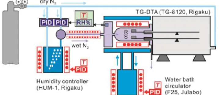
S1. Instrumental setup
Measurements of the mass-loss curves under controlled p(H2O) conditions were performed using a
controlled humidity TG–DTA system (HUM-TG, Thermoplus 2, Rigaku).84 Figure S1 shows the
system comprises a horizontally configured thermobalance (TG-8120, Thermoplus 2, Rigaku) with an electric furnace surrounded by a water jacket, a water circulator with a temperature controller (F-25, Julabo), a humidity controller (HUM-1, Rigaku), and a transfer tube with a temperature controller between the humidity controller and the thermobalance, and a dry N2 gas supply line
connected from a N2 gas cylinder equipped with a pressure regulator.
Figure S1. Overview of the controlled humidity TG–DTA system (HUM-TG, Thermoplus 2, Rigaku).
Before measurement, the electric furnace of the thermobalance and an anterior chamber connected to the furnace tube were warmed up by circulating water of controlled constant temperature ranging from 293–353 K. A purge gas of dry N2 flowed through at a rate of 50 cm3 min-1 from the back of the balance
system. After the sample was set on the sample holder in the thermobalance, the sample was heated to 353 K at a heating rate of 5 K min-1 under a stream of dry N
2 gas at 400 cm3 min-1 introduced from the
forefront of the furnace via the anterior chamber and held at the programmed temperature for 30 min. Immediately after the sample reached the programmed temperature, the dry N2 gas from the front of
the furnace was switched to wet N2 gas at a controlled p(H2O) value. The wet N2 gas was generated in
the humidity controller by bubbling N2 gas in a temperature controlled water bath. The wet and dry N2
gases were mixed and transferred in the anterior chamber of the furnace at a rate of 400 cm3 min-1 via
a transfer tube heated at a temperature ranging from 308–373 K. In the anterior chamber, the relative humidity and temperature of the wet N2 gas were continuously measured, with the relative humidity
signal returned to the humidity controller for the control of flowrates of the wet and dry N2 gases to be
mixed, so as to regulate the relative humidity in the anterior chamber to be the programmed value. The
p(H2O) value of the wet N2 gas in the anterior chamber was calculated using the temperature and
relative humidity values. The wet N2 gas with the controlled p(H2O) value was passed over the sample
and ejected through the part of the furnace linked to the balance room, together with the dry N2 gas
that purged the balance room. After stabilized the measurement system under a stream of wet N2 gas
with the controlled p(H2O) value for 30 min, the mass-loss curves for the thermal decomposition of
the Mg(OH)2 sample were obtained at the set p(H2O) value under isothermal and linear nonisothermal

![Risiko- & [und] Schutzfaktoren der psychischen Gesundheit humanitärer Einsatzhelfer : eine systematische Literaturübersicht](data:image/gif;base64,R0lGODlhAQABAIAAAP///wAAACH5BAEAAAAALAAAAAABAAEAAAICRAEAOw==)