Use of Parallel Computers in Rational Design of
Redundant Sensor Networks
C. Gerkens, G. Heyen
Laboratoire d’Analyse et de Synthèse des Systèmes Chimiques Université de Liège, Sart-Tilman B6A, B-4000 Liège (Belgium)
Tel: +32 4 366 35 23 Fax: +32 4 366 35 25 Email: C.Gerkens@ulg.ac.be
Abstract
A general method to design optimal sensor networks able to estimate process key variables within a required precision was recently proposed. This method is based on the data reconciliation theory and the sensor network is optimised thanks to a genetic algorithm. To reduce the solution time, two ways of parallelizing the algorithm have been compared: the global parallelization and the distributed genetic algorithms. Both techniques allow reducing the elapsed time but the second one is more efficient.
Keywords: parallelization, genetic algorithm, sensor network, data reconciliation, MPI
1. Problem position
Chemical processes must be efficiently monitored to allow production accounting as well as for the enforcement of safety and environmental rules. Process control can only take place if a suitable sensor network is installed on the plant. However most measurements are erroneous. Moreover some variables can not directly be measured by a sensor, such as for example compressor or turbine efficiency, catalyst deactivation or reaction conversion.
Uncertainty due to random measurements errors can be reduced when redundant measurements are available. Data reconciliation allows to correct measurements and to access their reliability; simultaneously it provides estimates of unmeasured variables and their uncertainty (Heyen et al., 1996). However the accuracy of the estimates and the cost of the measurements system are strongly influenced by the number, the location, the type and the precision of sensors. A general method to design the cheapest sensor network able to determine all the process key variables within a prescribed precision becomes therefore necessary.
This problem of measurements system design was first solved by Bagajewicz (Bagajewicz M.J., 1997) for non-linear mass balance equations and by Madron (Madron F., 1992) who used a graph oriented method. We developed recently a method that takes into account energy balances and non-linear equations (Heyen and Gerkens, 2002). The equations of the data reconciliation model are linearised at the nominal operating conditions, assuming steady state operation. The problem is formulated as an optimization problem whose objective function depends of the costs of sensors and the accuracy obtained for key variables. As the problem is usually multimodal and involves
many binary variables (presence or absence of sensors), it was solved by mean of a genetic algorithm (Goldberg, 1989).
This method was applied successfully to small and medium problems of about 200 to 600 variables. The time required to obtain the solution is about 10-15 minutes for an ammonia synthesis loop (198 variables) and about 4 hours for an acid acetic cracker that produces ketenes (618 variables) on aPentium II processor (333 Mhz). This time is too long to apply the algorithm to much larger problems. To reduce the solution time, the algorithm was parallelized by mean of the Message Passing Interface (MPI) (Gropp et al., 1999). Two parallelization methods, the global parallelization and the distributed genetic algorithms are discussed in this paper. Those techniques are compared for an ammonia synthesis loop.
2. Description of the genetic algorithm
Before being parallelized, our method was decomposed in four steps:
a. First of all a database for the sensors containing the accuracy, the range of measurement and the cost of each sensor is created, and a validation model of the process is built using Belsim-Vali III software. This software allows to export the linearised equations of the problem after computing a steady state solution for typical operating conditions.
b. Secondly the algorithm verifies that there exists a solution for the network containing all the sensors that can be implemented. If no feasible solution is found, the program stops and the problem should be defined in another way.
c. Thirdly, if the problem has a solution, the sensor network is optimised by mean of a genetic algorithm applying natural mechanisms of selection, one point crossing and jump mutation. The best chromosome is considered as the solution of the problem if it stays unchanged after a determined number of generations.
d. Finally, the solution is saved in a report file.
3. Parallelization
As they share the computing work between several processors, parallelization techniques allow reducing the solution time. However, this reduction of computing time must be done without increasing too much the computing resources. Parallelization techniques can be compared using a ratio, which takes into account the number of active processors, and the time required to obtain the solution.
Speed up Efficiency
Number of active processors
Time for 1 processor 1
Time for n processors Number of active processors =
=
The calculations were carried out on a cluster of identical Apple Power Mac G4 bi-processors.
3.1 Global parallelization
The global parallelization method consists of carrying out in parallel the evaluation of chromosomes fitness or the application of the genetic operator.
In the case of our algorithm, the evaluation of the objective function of all chromosomes of the population is the limiting step. Each chromosome evaluation requires two inversions of sensitivity matrix: first the non-singularity is checked assuming the physical property model is ideal. Afterwards a posteriori variances are estimated by inverting the sensibility matrix using non-ideal thermodynamic model. The size of those matrices is equal to the sum of the number of variables and the number of equations of the problem. That’s why the solution time of our algorithm increases much faster than the size of problems.
Chromosomes are evaluated independently from one another so that the algorithm was parallellized at that level. Evaluation of the fitness function for all chromosomes is distributed among available processors. Each chromosome handles completely the evaluation. Thus the maximum useful number of processors is equal to the size of the chromosome population. The other tasks of the algorithm (chromosomes distribution, population evolution) are completed by the master processor only: as they consist of rapid operations, losses of efficiency they cause are not important. As all processors need some information about the chemical process that is studied, the first generation of chromosomes is evaluated simultaneously by all active processors (this involves all
Validable me asure me nt syste m 0 50 100 150 200 250 300 350 0 0.2 0.4 0.6
1/ proce ssors numbe r
T im e (s ec ) 50 60 70 80 90 100 E ff ic ie n cy (% )
Master time Elapsed time
Efficiency
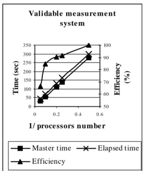
Figure 1: global parallelization:
determination of a validable
measurement system in the case of an ammonia synthesis loop
Observable measurement system in case of failure of one sensor
0 200 400 600 800 1000 1200 1400 1600 1800 2000 0 0.01 0.02 0.03 0.04 0.05 0.06 1/ processors number T im e ( se c ) 50 55 60 65 70 75 80 85 90 95 100 E ff ic ie n c y ( % )
Master time Elapsed time
Efficiency
Figure 2: global parallelization: determination of a measurement system that is observable when one sensor fails in the case of an ammonia synthesis loop
initialisation and processing the problem definition files). Global paralelization was carried out in two ways:
a. First of all the number of active processors was chosen lower or equal to the number of chromosomes to be evaluated. In that case, it appears that the efficiency is better when the number of active processors is a divisor of the number of chromosomes so that each processor has to handle the same number of chromosomes. As can be seen on figure 1, in the case of an ammonia synthesis loop, the elapsed time required to obtain the optimal validable measurement system and the time of the master processor is inversely proportional to the number of active processors. The efficiency decreases rapidly when the number of active processors approaches the number of chromosomes. This can be explained by considering how the fitness function is evaluated for a given sensor selection. First one has to checkif the sensor arrangement is feasible by verifying that the jacobian matrix of the model equations is not singular. When this is the case, the processor being in charge of an evaluation remains idle while the others processors go on evaluating the variances for all state variables.
b. Secondly the number of active processors was taken higher than the number of chromosomes. This case can only be considered when designing a measurement systems that remain observable in case of one sensor failure. The fitness function has to be evaluated for all sensor configurations obtained by removing one sensor from the current selection, and this work can be distributed among several processors. As can be
Influence of the number of 10 chromosoms sub-populations 0 500 1000 1500 2000 0 2 4 6 8 10
Num ber of sub-populations
Total number of iterations Master time (sec) Objectif function
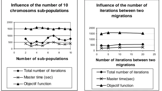
Figure 3: distributed genetic algorithm: influence of the number of sub-populations in the case of an ammonia synthesis loop
Influence of the number of iterations between two
migrations 0 500 1000 1500 2000 0 5 10 15 20 25
Number of iterations between two migrations
Total number of iterations Master time(sec) Objectif function
Figure 4:distributed genetic algorithm:
influence of the number of iterations between two migrations in the case of an ammonia synthesis loop
seen on figure 2 for the ammonia synthesis loop, the calculation times are still inversely proportional to the number of processors and the efficiency falls when the number of processors comes close to the number of evaluations for the population.
The clock time required to design a validable measurements networks is less than one minute for the ammonia synthesis loop (198 state variables and 117 possible sensors) and about fifteen minutes for an acetic acid cracker to produce keten (618 state variables 269 possible sensors).
3.2 Distributed genetic algorithm
In order to improve the efficiency, we attempted parallelizing the calculation by means of of distributed genetic algorithms (Herrera F. et al., 1999).
The method of distributed genetic algorithms consists of sharing the chromosomes in several populations, which are independent from one another. Those sub-populations evolve thanks to their own genetic algorithm. Periodically some chromosomes move between the different sub-populations thanks to a migration operator. In each sub-population, the migrating chromosomes are chosen and distributed at random. The chromosomes that are replaced are also taken at random. That random choice allows keeping most of the information contained in the global population. The four parameters that have to be specified are discussed here below:
a. The size of sub-populations: sub-populations of 10 and 20 chromosomes were studied. It appeared that the time required by sub-populations of 10 chromosomes to obtain similar solutions is twice smaller than the one for sub-populations of 20 chromosomes. So all the other
tests were performed with
sub-populations of 10
chromosomes;
b. The number of migrating chromosomes in each sub-population: the value of this parameter was taken equal to 2 what correspond to 20 % of sub-populations’ chromosomes; c. The number of sub-populations: as can be seen on figure 3, it is not possible to obtain a correlation between computing resources (or the number of sub-populations) and the solution time. A value of five was kept because it seems to be the best compromise; d. The number of iterations of
Time comparison between global parallelistaion and distributed
algorithm 0 100 200 300 400 500 600 700 800 0 1 2 3 4 5 6 7 8 9 10
Number of processors or sub-populations T im e ( s e c )
Global parallelisation : master time Global parallelisation : elpased time Distributed algorithm : master time Distributed algorithm : elapsed time
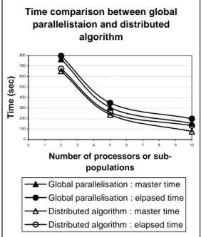
Figure 5: time comparison between global
the genetic algorithms between two migrations: the value of five found in the literature agrees with the results presented on figure 4.
The elapsed and master times for global parallelization and distributed genetic algorithm are compared on figure 5. It can be seen that distributed genetic algorithm requires less time that global paralelization. Furthermore, the values of objective function are better in the case of distributed genetic algorithm.
4. Conclusion and future work
The parallelization of the proposed method of design of optimal sensor networks allows to obtain validable measurements sets within an acceptable time for small and medium problems. For larger size problem, solutions time is still expected to be very important so that treating plants like refineries could not be considered nowadays. However suboptimal solutions of practical use can be obtained by considering individual plant sections.
Two parallelization methods were tested: both allow reducing the solution clock time but the distributed genetic algorithms appear superior in all points of view for all cases we considered.
The algorithm could also be parallelized by means of dynamic populations such that each chromosome would have his own life time that would be managed by the master processor.
References
Madron F., 1992, « Process Plant Performance Measurement and Data Processing for Optimisation and Retrofits », section 6.3, Ellis Horwood
Bagajewicz M.J., 1997, « Process Plant Instrumentation: Design and Upgrade », chapter 6, Technomic Publishing Company
Heyen G., Maréchal E., Kalitventzeff B., 1996, « Sensitivity Calculations and Variance Analysis in Plant measurement Reconciliation », Computers and Chemical Engineering, volume 20S, 539-544
Goldberg D.E., 1989, « Genetic Algorithms in Search, Optimization and Machine Learning », Addison-Wesley
Gropp W., Lust E., Skjellum A., 1999, « Using MPI: Portable Parallel Programming with the Message Passing Interface », Second Edition, The MIT Press
Herrera F., Lozano M., Moraga C., november 1999, « Hierarchical Distributed Genetic Algoritms », International Journal of Intelligent Systems, Volume 14 (11), 1099-1121
Heyen G., Gerkens C., 2002, « Application d’algorithmes génétiques à la synthèse de systèmes de mesure redondants », proceedings of SIMO 2002 Congress, Toulouse (24-25 october 2002)