Faculty of Applied Sciences
Department of Electrical Engineering and Computer Science
PhD dissertation
A walk into random forests
Adaptation and application
to Genome-Wide Association Studies
Author
Vincent Botta
Supervisor
Prof. Louis Wehenkel
Summary
Understanding underlying mechanisms of common diseases is one of the major goals of current research in medicine. As most of these disorders are linked to genetic factors, identification of the associated variants forms an excellent strategy towards the elucidation of molecular and cellular dysfunctions, and in fine could lead to better personalised diagnostics and treatments.
Genome-Wide Association Studies (gwas) aim to discover variants spread over the genome that could lead, in isolation or in combination, to a particular trait or an unfortunate phenotype such as a disease. The basic idea behind these studies is to statistically analyse the genetic differences between groups of healthy (controls) and diseased (cases) individuals. Advances in genetic marker technology indeed allow for dense genotyping of hundreds of thousands of Single Nucleotide Polymorphisms (snps) per individual. This allows to characterise representative samples composed of several hundreds to several thousands of cases and controls, each one characterised by up to a million of genetic markers sampling the genomic variations among these individuals.
The standard approach to genome wide association studies is based on univariate hypothesis tests. In this approach each genetic marker is analysed in isolation from the others, in order to assess its potential association with the studied phenotype, in practice by the computation of so-called p-values based on some statistical assumptions about the data-generation mechanism. Because of the very high ratio between the large number of snps genotyped and the limited number of individuals, multiple-testing corrections need to be applied when carrying out these analyses, leading to reduced statistical power.
While this standard approach has been at the basis of many novel loci unravelled in the last years for several complex diseases, it has several intrinsic limitations. A first limitation is that this approach does not directly account for correlations among the explanatory variables. A second intrinsic limitation of gwas is that they can’t account for genetic interactions, i.e. causal effects that are only observed when specific combinations of mutations and/or non-mutations are present at the same time. The third limitation of univariate approaches is that they do not directly allow to assess the genetic risk, since many of the identified markers (with similarly small p-values) actually account for the same underlying causal factor: exploiting their information to predict the genetic risk is hence far from straightforward.
Within bioinformatics, machine learning has actually become one of the major potential sources of progress. As a matter of fact, biology has become nowadays one of the main drivers of research in ma-chine learning, and is by itself already a very competitive research field.
Among the subfields of machine learning, supervised learning and its extensions such as semi-supervised learning, stand out as the most mature and at the same time most rapidly evolving area of research. Within this context, the purpose of this thesis was to study the application of random forest types of methods to genome wide association studies, with the twofold goal of (i) inferring predictive models able to asses disease risk and (ii) to identify causal mutations explaining the phenotype. The choice of this family of methods was originally motivated by the fact that these methods are a priori well suited for that kind of analysis due to some of their interesting properties. They are indeed able to deal efficiently with very large amounts of data without relying on strong assumptions about the underlying mechanisms linking genetic and environmental factors to phenotypes, and they can also provide interpretable information, in the form of scorings and/or
In the first part of this manuscript, we analyse the state-of-the art in the application field of genome wide association studies and in supervised machine learning, and subsequently describe in details the three tree-based ensemble methods that we have implemented and applied in our research; in Part II, we report our empirical investigations, in three successive steps, namely i.) a preliminary study on simulated datasets yielding controlled conditions with known ground-truth and allowing for a first sanity check of the T-Trees methods, in ideal conditions; ii.) a detailed study on a given real-life dataset concerning Crohn’s disease, where we try to understand the main features of the three different algorithms in terms of predictive accuracy and capability of identification of relevant genetic information, and their sensitivity with respect to various kinds of quality control procedures and algorithmic parameters; iii.) a systematic replication study, where we confirm, on 7 different datasets from the Wellcome Trust Case Control Consortium, the main outcomes of our study on the Crohn’s disease, while using default parameter settings.
Remerciements
Durant ces dures années de labeur, de nombreuses personnes m’ont aidé, accompagné, épaulé, encouragé, soutenu ou tout simplement écouté. Toutes ces contributions, qu’elles soient scientifiques ou non, ont été déterminantes et souvent essentielles, pour le bon déroulement de cette épopée.
Parmi les essentiels, je commencerai par remercier Louis Wehenkel, promoteur de cette thèse, pour ses précieuses interventions, sa disponibilité et sa patience. La confiance et le respect qu’il m’a accordés m’ont permis d’évoluer et de découvrir le monde passionnant de la recherche. Nos nombreuses discussions ont plus que largement contribué à la bonne réalisation de ce travail. Toujours dans les essentiels, je remercie également Pierre Geurts, co-promoteur de ce travail, pour le partage de son expertise, sa disponibilité, ses nombreuses réponses éclairées et éclairantes, son dévouement et sa gentillesse.
Je remercie également les membres du jury de cette thèse qui ont dédié leur précieux temps à sa lecture et à son évaluation.
Ensuite, il y a les satellites, toutes ces personnes qui ont gravité, de près ou de loin, autour de cette recherche. Ceux avec qui j’ai eu l’occasion de partager et discuter, ceux qui ont élargi mes horizons et ouvert de nouvelles voies, ceux qui ont ajouté leur grain de sable et contribué, parfois sans s’en rendre compte, à la bonne conduite de mes recherches. Tom Druet pour ses précieuses remarques et le temps qu’il m’a accordé. Michel Georges pour tous ces échanges, parfois furtifs mais intenses et constructifs. J’ai également une pensée particulière pour l’impulsion qu’aura pu donner Sarah Hansoul à cette recherche. Je remercie aussi Gilles pour son coup de pouce efficace, indispensable et linéaire de la dernière ligne droite. Enfin, dans le désordre et non exhaustivement, je remercie Christophe, Jean-Fran¸cois, Fabien, Raphaël, Benjamin, Yannick, Olivier, ... et tous les collègues.
Après, il y a les persévérants. Ceux qui ont cru en moi sans en démordre une seconde, ceux qui ont été présents pour me maintenir sur la route, ceux qui m’ont entouré de leurs joies. Je ne remercierai sans doute jamais assez mes parents, mes deux merveilleuses soeurs, leurs magnifiques plus si petits bambins, mes grands-parents, Delphine, et Antoine (qui n’y est pas pour rien). Je remercie également Monique pour son authenticité et Jean-Claude pour son humour. Je remercie aussi tous ceux qui ont partagé leur amitié ainsi que de bien agréables instants (et surtout de bonnes bières) tout en refaisant le monde à mes côtés: Gérôme pour sa salsa, Samuel pour son coup de crayon sur la couverture, Jean-Marc pour son accent, Jérome pour ses anti-corps, ... et puis tous les autres.
Je remercie également l’Université de Liège, le GIGA, l’Institut Montefiore et le FNRS qui m’ont accueilli, couvert et chauffé quand il faisait froid.
Enfin, il y a Sylviane. Mon amour, mon étoile, mon refuge, mon pilier. Elle m’a accompagné tout au long de ce parcours. Jour et nuit, elle m’a soutenu et conforté. A mes côtés, elle a participé à cette épreuve et a vécu intensément les humeurs, bonnes et moins bonnes, qui accompagnent cette longue traversée du doctorat. Merci pour ta persévérance, ta force et la constance de ton amour. Merci de m’avoir attendu. Merci à toi, du fond du coeur.
Contents
1 Introduction 1
1.1 Motivations . . . 1
1.2 Approach to research . . . 3
1.3 Organization of the manuscript . . . 4
1.4 List of publications . . . 4
I
Background and Methods
5
2 Genome-Wide Association Studies 7 2.1 dna : 3 letters for 3 billions bases . . . 82.2 snp : 3 letters (again) for 3 values . . . 8
2.3 Genome-wide associations studies . . . 9
2.3.1 Thanks to linkage disequilibrium . . . 11
2.4 GWAS : how ? . . . 13
2.4.1 Quality controls . . . 14
2.4.2 Single-locus test of association . . . 16
2.4.3 A bit further . . . 19
3 Machines can learn 21 3.1 Datasets and notations . . . 22
3.1.1 Curse of Dimensionality . . . 22
3.2 The learning step . . . 23
3.3 The model evaluation step . . . 24
3.3.1 Prediction versus Interpretation . . . 25
3.3.2 Evaluation of the accuracy of binary classification models . . . 26
3.3.3 roc curves . . . 26
3.3.4 Cross-validation . . . 28
3.4 Summary . . . 29
4 Tree-based methods for GWAS 30 4.1 Motivations . . . 31
4.2 State-of-the-art in tree-based supervised learning . . . 32
4.2.1 Single Decision Trees . . . 32
4.2.2 Random Forests . . . 41
4.2.3 Extremely Randomized Trees . . . 45
4.3 Trees inside Trees . . . 47
4.3.1 Motivation . . . 47
4.3.2 Algorithm . . . 48
4.3.3 Evaluation of variable and group importances . . . 51
4.4 Extension to more quantitative or multiple phenotypes and environmental effects . . . 52
4.5 Related works . . . 52
4.6 Summary . . . 55 i
II
Validations
57
5 Comparison of RF and T-Trees on synthetic datasets 58
5.1 Synthetic ‘GWAS’ dataset generation . . . 59
5.1.1 Principle of the synthetic ‘genotype’ generation . . . 59
5.1.2 Principle of the synthetic ‘phenotype’ generation . . . 59
5.1.3 Comments . . . 60
5.2 Evaluation protocol . . . 60
5.3 Simulation results . . . 61
5.3.1 Sample efficiency of RF vs T-Trees in the context of a single causal block . . . 61
5.3.2 Robustness against label errors . . . 66
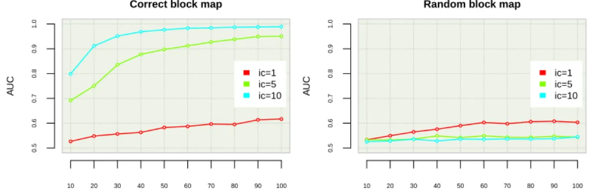
5.3.3 Influence of the quality of prior information about the block structure . . . 67
5.3.4 More than one causal block . . . 70
5.3.5 Modality, scale of measurement and number of categories . . . 70
5.4 Discussion . . . 74
6 The case of Crohn’s disease 76 6.1 Two dataset variants for Crohn’s disease . . . . 77
6.1.1 Predictions . . . 78
6.1.2 Identification of suceptibility loci . . . 88
6.2 A few experiments with linear models . . . 101
6.2.1 Sum of log odds ratio . . . 101
6.2.2 Globally trained linear models . . . 101
6.2.3 Preliminary analysis of the SNP rankings . . . 103
6.3 Discussion . . . 104
6.3.1 Importance of the preprocessings . . . 104
6.3.2 Methods . . . 105
7 Six other complex diseases 107 7.1 The six other diseases . . . 108
7.2 Comparison of the tree-based methods predictive power . . . 110
7.3 Variable importances analyses . . . 110
7.4 Overall remarks . . . 142
III
Conclusion
144
8 Closure 145 8.1 Epitome . . . 145 8.2 Main findings . . . 146 8.3 Further work . . . 1468.3.1 Tree-based supervised learning methods . . . 147
8.3.2 Genetical dissection of complex phenotypes by supervised learning . . . 147
8.3.3 Software development and implementation . . . 148
Appendices 150
A Additional data related to Chapter 6 150
B Additional data related to Chapter 7 156
List of Figures
2.1 One way for a mutation to influence phenotype. . . 9
2.2 From mutations to genotypes . . . 10
2.3 Overall principle of a gwas . . . 11
2.4 Direct versus indirect association . . . 11
2.5 Example of ld matrix . . . 13
2.6 Genotype cluster plot . . . 16
2.7 Graphical representation of a p-value . . . 18
2.8 An example of a Manhattan plot . . . . 18
3.1 The learning step . . . 23
3.2 Common model usage . . . 23
3.3 Evaluation of the generalization error . . . 25
3.4 Confusion matrix . . . 27
3.5 A roc curve . . . 27
3.6 An example of a 5-fold cross-validation . . . 28
4.1 A simple tree structure . . . 32
4.2 A simple example of decision tree . . . 33
4.3 Geometrical representation of a decision rule . . . 34
4.4 A degenerate tree . . . 39
4.5 Prediction with an ensemble of trees . . . 44
4.6 Overview of a T-Tree . . . 47
4.7 Difference between internal and external nodes . . . 49
4.8 Into the T-Tree test node . . . 49
4.9 General flowchart: building a decision tree . . . 56
4.10 General flowchart: building a forest . . . 56
5.1 Influence of learning set size, K and IC on the auc . . . 62
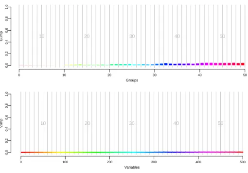
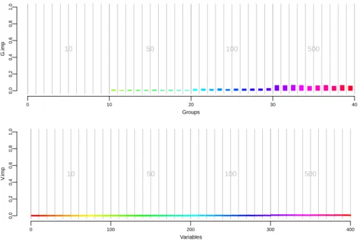
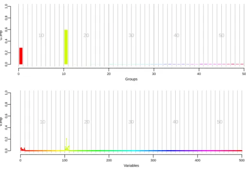
5.2 Variable and group importances with a small learning set . . . 63
5.3 Variable and group importances with a medium learning set . . . 64
5.4 Variable and group importances with a large learning set . . . 64
5.5 Comparison of three different ranking with a small learning set . . . 65
5.6 Comparison of three different ranking with a medium learning set . . . 65
5.7 Comparison of three different ranking with a large learning set . . . 65
5.8 Robustness against label errors . . . 66
5.9 Influence of bloc size . . . 68
5.10 Wrong block map experiment . . . 68
5.11 Ranking comparison with block of 20 variables and a strong IC . . . 69
5.12 Ranking comparison with block of 20 variables and a weak IC . . . 69
5.13 Experiment with more than one causal block . . . 71
5.14 Variable and group importances with three causal blocks . . . 72
5.15 Block modality experiment with no causal block . . . 72 iii
5.16 Blocks of higher modality experiment with no causal block . . . 73
5.17 Block modality experiment with one causal block . . . 73
5.18 Block modality experiment with two causal blocks . . . 74
6.1 Random Forests: influence of T , K and Nminon CDwtccc . . . 79
6.2 Random Forests: influence of T , K and Nmin on CDibd. . . 80
6.3 Random Forests dataset comparison: influence of Nmin. . . 80
6.4 Extra-Trees: influence of T , K and Nminon CDwtccc . . . 81
6.5 Extra-Trees: influence of T , K and Nminon CDibd . . . 82
6.6 Extra-Trees dataset comparison: influence of Nmin . . . 83
6.7 T-Trees IC = 10: influence of T , K and Nmin on CDwtccc . . . 84
6.8 T-Trees IC = 10: influence of T , K and Nmin on CDibd . . . 85
6.9 T-Trees dataset comparison: influence of Nmin . . . 85
6.10 T-Trees: influence of the internal complexity . . . 86
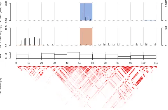
6.11 A glance at the 100 first variables on CDwtccc. . . 90
6.12 A glance at the 100 first variables on CDibd . . . 91
6.13 A closer look at the nine reported regions . . . 92
6.14 Two more regions detected by our tree based methods . . . 92
6.15 The region 2p12 on CDibd. . . 93
6.16 The region 7q31 on CDibd. . . 93
7.1 Markers inclusion/exclusion for the 3 CD datasets . . . 109
7.2 A glance at the 100 first variables on BDqc . . . 113
7.3 A glance at the 100 first variables on BDwtccc. . . 114
7.4 A glance at the 100 first variables on CADqc . . . 117
7.5 A glance at the 100 first variables on CADwtccc . . . 118
7.6 A glance at the 100 first variables on CDqc . . . 122
7.7 A glance at the 100 first variables on CDwtccc. . . 126
7.8 A glance at the 100 first variables on HTqc. . . 127
7.9 A glance at the 100 first variables on HTwtccc . . . 128
7.10 A glance at the 100 first variables on RAqc. . . 131
7.11 A glance at the 100 first variables on RAwtccc . . . 132
7.12 A glance at the 100 first variables on T 1Dqc . . . 135
7.13 A glance at the 100 first variables on T 1Dwtccc . . . 136
7.14 A glance at the 100 first variables on T 2Dqc . . . 138
7.15 A glance at the 100 first variables on T 2Dwtccc . . . 139
A.1 A closer look at the nine reported regions (normalised vertical axis) . . . 151
B.1 BD: The 100 first variables positioned . . . 157
B.2 CAD: The 100 first variables positioned . . . 158
B.3 CD: The 100 first variables positioned . . . 159
B.4 HT: The 100 first variables positioned . . . 160
B.5 RA: The 100 first variables positioned . . . 161
B.6 T 1D: The 100 first variables positioned . . . 162
B.7 T 2D: The 100 first variables positioned . . . 163
C.1 Different auc curve profiles with three score measures on CDwtccc . . . 164
C.2 Different auc curve profiles with three score measures on CDibd . . . 164
C.3 Minor allele frequencies in the 1000 first variables on CDwtccc . . . 165
List of Tables
2.1 The notion of departure from the uncorrelated state . . . 12
2.2 Full genotype table for a general genetic model : 2 × 3 table . . . 16
2.3 Expected genotype counts . . . 17
2.4 Dominant model . . . 19
2.5 Recessive model . . . 19
4.1 Example of data for a credit card marketing problem . . . 33
4.2 The contingency table from which score measures are derived . . . 38
5.1 List of investigated phenotypes . . . 70
6.1 Random forest versus Extra-Trees: auc comparison . . . 83
6.2 T-Trees: aucs versus internal complexity . . . 86
6.3 T-Trees: block map and internal complexity influence . . . 87
6.4 Summary table: comparison between the three methods . . . 87
6.5 T-Trees: contiguous versus randomised blocks . . . 88
6.6 The nine wtccc confirmed regions . . . 88
6.7 The 6 common haplotype found in the 2p12 and the 7q31 regions. . . 91
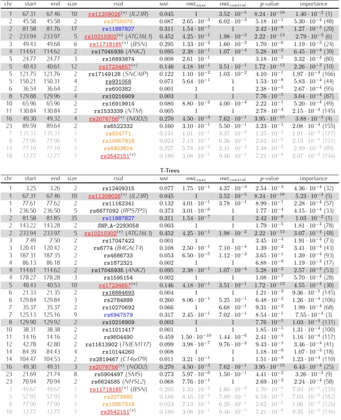
6.8 The 20 first variables according to the random forest on CDibd . . . 94
6.9 The 20 first variables according to the T-Trees on CDibd. . . 95
6.10 Using only some regions on CDibd: aucs . . . 96
6.11 Using only some regions on CDwtccc: aucs . . . 97
6.12 CDibd: lists of regions identified by the Random Forests and the T-Trees methods. . . 99
6.13 Rare and common variants: aucs . . . 100
6.14 With and without chromosome X . . . 100
6.15 aucs obtained with the “log odds ratio” methods on the two CD datasets. . . 101
6.16 aucs obtained with linear models learnt by stochastic gradient descent . . . 102
6.17 Comparison of aucs between the tree-based and the linear models. . . 103
7.1 The 7 diseases from the WTCCC dataset: naming conventions . . . 108
7.2 Quality control filters influence . . . 109
7.3 Numbers of markers being excluded by the wtccc in our dataset versions . . . 109
7.4 Predictive power: auc comparisons . . . 110
7.5 BDqc: lists of regions identified by the Random Forests and the T-Trees methods. . . 115
7.6 BDwtccc: lists of regions identified by the Random Forests and the T-Trees methods. . . 116
7.7 CADqc: lists of regions identified by the Random Forests and the T-Trees methods. . . 119
7.8 CADwtccc: lists of regions identified by the Random Forests and the T-Trees methods. . . . 120
7.9 CDibd: lists of regions identified by the Random Forests and the T-Trees methods. . . 123
7.10 CDqc: lists of regions identified by the Random Forests and the T-Trees methods. . . 124
7.11 CDwtccc: lists of regions identified by the Random Forests and the T-Trees methods. . . 125
7.12 HTqc: lists of regions identified by the Random Forests and the T-Trees methods. . . 129
7.13 HTwtccc: lists of regions identified by the Random Forests and the T-Trees methods. . . 130
7.14 RAqc: lists of regions identified by the Random Forests and the T-Trees methods. . . 133
7.15 RAwtccc: lists of regions identified by the Random Forests and the T-Trees methods. . . 134
7.16 T 1Dqc: lists of regions identified by the Random Forests and the T-Trees methods. . . 137
7.17 T 1Dwtccc: lists of regions identified by the Random Forests and the T-Trees methods. . . 137
7.18 T 2Dqc: lists of regions identified by the Random Forests and the T-Trees methods. . . 140
7.19 T 2Dwtccc: lists of regions identified by the Random Forests and the T-Trees methods. . . 141
A.1 The 20 first variables according to the random forest on CDwtccc . . . 152
A.2 The 20 first variables according to the p-values on CDwtccc . . . 153
A.3 The 20 first variables according to the p-values on CDibd . . . 154
A.4 T-Trees variable importances in chromosome region on CDwtccc . . . 155
List of Algorithms
1 A decision tree is a cascade of if-then-else . . . 33
2 Growing a fully developed decision tree . . . 37
3 The Random Forests algorithm . . . 43
4 Building one tree in a Random Forests . . . 43
5 The Extra-Trees algorithm . . . 46
6 Building one tree in the Extra-Trees . . . 46
7 The T-Trees algorithm . . . 50
8 Building one tree in the T-Trees . . . 50
9 The T-Trees splitting rule . . . 51
10 Building the trees inside the T-Trees test nodes . . . 51
Introduction
In this chapter we successively discuss the motivations of our research, present the overall approach used to work, and then outline the structure of the rest of this manuscript and conclude by stating our personal contributions and by providing an annotated list of our publications.
1.1
Motivations
Understanding underlying mechanisms of common diseases, such as cancer, cardiovascular diseases, inflam-matory and allergy disorders, is one of the major goals of current research in medicine. As most of these disorders are linked to genetic factors, identification of the associated variants forms an excellent strategy towards the elucidation of molecular and cellular dysfunctions, and in fine could lead to better personalized diagnostics and treatments.
Genome-Wide Association Studies (gwas) aim to discover variants spread over the genome that could lead, in isolation or in combination, to a particular trait or an unfortunate phenotype such as a disease [Man10, TKTJ11, LCVK11, Wel07]. The basic idea behind these studies is to statistically analyze the genetic differences between two populations: a group of healthy individuals (the controls) versus a group of sick ones (the cases). Advances in genetic marker technology indeed allow for dense genotyping of hundred of thousands of Single Nucleotide Polymorphisms (snps) per individual. This allows to characterize, at an acceptable cost, representative samples composed of several hundreds to several thousands of cases and controls, each one characterized by up to a million of genetic markers sampling the genomic variations among these individuals.
In addition to the genetic measurements and the binary case/control classification, the individuals may also be characterized by additional information, such as for example, additional phenotypes refining their biological condition, and a multitude of environmental factors that may interact with genetic ones and often significantly impact disease status. Furthermore, meta-datasets may be constructed by merging information from several independent studies about the same or related diseases [B+08, T+12b, S+12].
The very high practical importance of all theses studies, and the rapidly growing amount and complexity of the data generated by all these experiments raise many interesting questions for their analysis, and hence foster intensive research on the development of novel bioinformatics and statistical methodologies to help extracting in a more effective way the relevant information from these datasets.
The standard approach to genome wide association studies is based on univariate hypothesis tests. In this approach each genetic marker is analyzed in isolation from the others, in order to assess its potential association with the studied phenotype, in practice by the computation of so-called p-values based on
some statistical assumptions about the data-generation mechanism [Bal06, M+08, BCB04]. Because of
the very high p/n ratio in gwas (here p denotes the number of explanatory variables, i.e. the number of snps genotyped, while n denotes the sample size, i.e. the number of individuals used as cases and
controls), multiple-testing corrections need to be applied when carrying out these analyses, leading to reduced statistical power.
While this standard approach has been at the basis of many novel loci unravelled in the last years for several complex diseases, it has several intrinsic limitations.
A first limitation is that this approach does not directly account for correlations among the explanatory variables, while in the context of gwas this correlation is often very strong, in particular due to the fact that genetic mutations are transmitted from parents to children through a combination of chromosome replication and cross-over, which leads to a high probability that mutations that are closely located on a dna strand are inherited in combination, hence leading to strong correlations among closely located genetic markers. Apart from this unavoidable physical correlation, correlations among different markers may also appear as artefacts induced by the experiment design (sample selection, experimental batches, imputations of missing variables) routinely found in the datasets used for gwas. The net result is that p-value based marker rankings need to be carefully analyzed by hand and subsequently experimentally replicated and validated before they can be confirmed as pin-pointing to genuine causal effects. This situation led to a recurring difficulty in reproducing findings published in the literature and made the scientific community become extremely cautious [INTCI01] and demanding on the soundness of the statistical approaches used in gwas.
A second intrinsic limitation with the univariate approaches to gwas is that they can’t account for genetic interactions, i.e. causal effects that are only observed when specific combinations of mutations and/or non-mutations are present at the same time. Even though opinions are divided [HGV08, ZHSL12], such potential epistatic effects should however be taken into account in order to increase the power of the statistical analyses. Furthermore, it is not unlikely that many genetic factors are in some way coupled with environmental factors, and taking these couplings systematically into account is as well beyond the capabilities of simple univariate approaches.
The third limitation of univariate approaches is that they do not directly allow to assess the genetic risk, since many of the identified markers (with similarly small p-values) actually account for the same underlying causal factor: exploiting their information to predict the genetic risk is hence far from straightforward, even more so if we want to take into account potential gene-gene or gene-environment interactions.
Since the mid-eighties, the field of machine learning has emerged at the intersection of algorithmics and statistics. The overall goal of the field is to design and theoretically characterize algorithms to extract in a reproducible way relevant information from observational data. The field is driven by a large diversity of applications, such as text mining [FS06], image analysis [MGW09, MGW07], extraction of knowledge from the internet [CMFF10], analyzing data from experimental sciences such as astronomy [B+09], earth monitoring
[K+11], high energy physics [P+12b], and - last but not least - biology and medicine [MAW10]. Within
bioinformatics, machine learning has actually become one of the major potential sources of progress, as one can contemplate from the growing number of conferences and journals that focus on the application of machine learning to biology. As a matter of fact, biology has become nowadays one of the main drivers of research in machine learning, and is by itself already a very competitive research field.
Among the subfields of machine learning, supervised learning and its extensions such as semi-supervised learning, stand out as the most mature and at the same time most rapidly evolving area of research: the general statistical theory underlying the analysis of supervised learning algorithms has been established at the end of the last century [PRMN04, Vap98a], and in the meantime several powerful paradigms have been developed allowing to leverage supervised learning to a very broad class of problems. Among these supervised learning methods, both kernel-based models [lS02] and tree-based models stand out. In particular, random forest types of methods [Bre01, GEW06], have been shown to provide state-of-the-art results in many applications (e.g., image analysis, bioinformatics, reinforcement learning, etc.), specially in terms of their excellent accuracy vs computational complexity compromise.
Within the above context, the subject of this thesis was defined a few years ago, in the establishment of a collaboration between the research unit in Systems and Modeling of the Department of Electrical
Engineering and Computer Science, on the one hand, and the research unit in Animal Genomics of the Faculty of Veterinarian Medicine, on the other hand. These groups were and still are respectively active in machine learning, and specifically in tree-based supervised learning, and in genome wide association studies, and specifically the study of complex genetic diseases.
The purpose of our work was to study the application of random forest types of methods to genome wide association studies, with the twofold goal of (i) inferring predictive models able to asses disease risk and (ii) to identify causal mutations explaining the phenotype. The choice of this family of methods was originally motivated by the fact that these methods are a priori well suited for that kind of analysis due to some of their interesting properties. They are indeed able to deal efficiently with very large amounts of data without relying on strong assumptions about the underlying mechanisms linking genetic and environmental factors to phenotypes, and they can also provide interpretable information, in the form of scorings and/or rankings of snps so as to help in the identification of causal genetic loci.
1.2
Approach to research
Given the limitations of the standard approach discussed in the preceding section, and the acknowledged capability of tree-based methods to handle complex problems in a very flexible way, it is of interest to investigate whether and how these methods could be used in order to improve on univariate approaches in the context of gwas.
To carry out this investigation, we have worked during our thesis along the following work plan:
• We have started our work by implementing our own software for supervised learning with ensembles of
trees; to do so we have been inspired by the experience in the Systems and Modeling team, but we have developed our own software from scratch in order to facilitate later adaptations and benchmarkings.
• At the onset of our thesis, we have participated in some GWAS carried out in the companion group
of animal genetics, to become familiar with the nature of the datasets, and most importantly with the quality control and other preprocessings needed prior to statistical analysis.
• We then have applied standard random forest types of algorithms to some synthetic and real-life
datasets, in order to gain some first hands-on experience. This also led to some improvements in our software implementation, so as to make it sufficiently efficient (memory, cpu time, adaptation to grid environment) to handle very big datasets.
• In order to cope with the correlation structure implied by linkage disequilibrium, we have designed
a novel tree-based ensemble method called T-Trees and tested it on synthetic data. The method is based on the segmentation of the vector of snps into blocks of fixed size along the genome, and then uses the snps inside each block in a homogenous way by first selecting at each tree node a block and then jointly exploiting the snps inside this block to create a split. We found that it yields both improved predictive accuracy and a better precision in the detection of causal loci.
• Finally, we have carried out a systematic large-scale empirical investigation based on
state-of-the-art and publicly available gwas datasets about several human diseases. This study allowed us to better understand the features of tree-based ensemble methods in real-life conditions, in particular by identifying the role played by the interaction of rare variants with some pathological behaviors of the score measures used for tree induction. We also assess in this study the effect of quality control on the apparent predictive power of the induced classifiers, by comparing results according to different quality control procedures. The results found in this study should help other machine learning researchers to more effectively analyze their results when using complex black-box procedures such as tree-based ensemble methods, and at the same time help biologists to gain confidence in these results.
1.3
Organization of the manuscript
The main body of the manuscript is divided in two parts.
In part 1, we start by describing the state-of-the-art in genome wide association studies (Chapter 2), and then provide in Chapter 3 the required background in supervised machine learning. Chapter 4 gives a precise description of the algorithms that we have developed and applied in this work.
In part 2, we present our experimental results. We start, in Chapter 5 by analyzing the behavior of standard random-forest types of methods and our proposed method called T-Trees on synthetic datasets, where the ground truth is known, and where we can easily vary experimental conditions (noise level, number of samples etc.) In chapter 6, we then provide detailed results on the real-life Crohn’s disease (cd) dataset from the wtccc [Wel07], and link our results with the scientific literature. Chapter 7 complements our empirical study by investigating the six remaining datasets related to other diseases provided by the wtccc. Some complementary simulations results are collected in the appendices.
Finally, we conclude by discussing in a retrospective way our findings and by suggesting future directions of research.
1.4
List of publications
In [BGHW08a, BGHW08b], we started to tackle the problem of correlated descriptors in gwas by considering two different representations of the input data: the raw genotypes described by a few thousand to a few hundred thousand discrete variables each one describing a single nucleotide polymorphism and, on the other hand, haplotype block contents represented by the combination of 10 to 100 adjacent genotypes. The blocks were defined by the HapMap hotspot lists. We adapted the Random Forests to exploit those blocks and compared the results with the use of raw genotypes in terms of predictive power and localization of causal loci. The adaptation consisted in modifying the splitting rule based on estimation of the conditional probability that the observed haplotype is drawn from the population of cases (reps. controls) reaching the current node (assuming class conditional independence of the snps in the block). That methodology was applied on simulated datasets with one or two interacting causal mutations. We obtained marginally superior results with our adaptation of the state-of-the-art tree-based method than their direct application to the raw genotype data. That first contribution opened the path we followed in the present thesis.
Also, at the beginning of my PhD, I had the opportunity to develop a graphical interface allowing biologists to annotate images and perform different measurements while extracting subimages used as inputs for tree-based automatic image classification. That work lead to a publication [G+08b] related to the effectiveness of inhaled doxycycline to prevent allergen-induced inflammation in a mouse model of asthma.
An article [BLGW13] presenting the core results of this thesis, namely the T-Trees algorithms, and its application to seven real gwas datasets is under preparation and will be submitted to a journal. In this paper, the capabilities of various tree-based ensemble methods to assess disease risk and to localize causal mutations are evaluated. We are also preparing a short technical note to be submitted to a bioinformatics journal, where we present our findings about the impact of the normalisation of the splitting-criterion used in random forests methods and their bias towards markers with small minor allele frequencies (appendix A.1).
Background and Methods
Genome-Wide Association Studies
Contents
2.1 dna : 3 letters for 3 billions bases . . . 8
2.2 snp : 3 letters (again) for 3 values . . . 8
2.3 Genome-wide associations studies . . . 9
2.3.1 Thanks to linkage disequilibrium . . . 11
2.4 GWAS : how ? . . . 13
2.4.1 Quality controls . . . 14
2.4.2 Single-locus test of association . . . 16
2.4.3 A bit further . . . 19
Humans are unique but genetically 99% equal. The remaining 1% of genetic differences participate in their rich diversity. Deoxyribonucleic acid (dna) depicts the essential information needed for building up a human living from the biological point of view. This genetic material can be seen as a linear code underlying the development, the functioning and the reproduction of organisms. Nevertheless, some coding errors may occur which, unfortunately, could cause dysfunction at many levels and eventually lead to diseases. The aim of genome-wide association studies is to locate genetic differences between two sub-populations that are responsible of the differences of one or several phenotypes observed between these sub-populations, and in particular that are related to complex genetic diseases.
This chapter first aims at providing a gentle introduction to the field of genome-wide association studies to non specialists. On the way, we will also present and discuss the current state-of-the-art in terms of statistical analysis techniques commonly used in this context.
2.1
dna : 3 letters for 3 billions bases
All humans have a sequence of roughly 3 billion dna bases spread over their 23 pairs of chromosomes. dna sequences can be viewed as a code containing genetic instructions.
From the informatics viewpoint, dna is essentially a very long linear string built over an alphabet of four different letters defined by chemical bases (or nucleotides) : A, C, T, G. Almost every cell of an organism contains two copies of this dna string and this information is transmitted in a quite reliable way from one cell to its daughters, and from one individual to its off-springs (actually exactly one half from both parents). Indeed, the genetic machinery responsible of dna replication is quite robust, and thanks to coding redundancy and error-correction mechanisms, the genetic information encoded by dna strands is normally reproduced with great fidelity.
However, during the replication process, errors may occur over time and survive in the offspring (cell lines and/or sub-populations), for example by changing one base to another at some positions in the code, or by yielding multiple copies of some dna subsequence. If we screen the genetic material of a sample of individuals of a population, at a position where such a mutation phenomenon occurred in the past, we will therefore observe that some individuals (typically a large majority of them) are holding the original genetic material, the so-called wild type, while others (typically a small minority) hold the mutant variant.
Among the various types of mutations that may occur, we focus in this thesis on point-wise mutations characterized by the change of a single letter (a replacement, a deletion, or an insertion) in the dna string. The resulting genetic variability is called Single Nucleotide Polymorphism (snp) and its alternate forms observed in the population are called alleles; in most of the cases, an snp is characterized by only two alleles which translate into three different combinations for diploid organisms.
snps are the most abundant source of genetic variation (aside from structural variations) within the human genome, notably because many of these appear in non-coding regions. (this is the redundant code defining the mapping between dna strings and protein sequences). From recent genetic surveys, it is known that these snps occur approximately once every 100 to 300 base-pairs on the average. The International HapMap Project [The03] has studied these variations and has identified about ten million snps (where the rarer snp allele has a frequency of at least 1%) in three sub-populations of humans (Europeans, Africans and East Asians). In the continuity, the 1000 Genomes Project [G+10] sequenced the genomes of more than
1000 people to obtain a more detailed and comprehensive catalogue of human genetic variation. The 1000 Genomes data are available to the scientific community. They can be used, for example, to impute genotypes not directly typed thus avoiding important genotyping costs.
Since genetic material is transmitted in a way such that nearby bases are transmitted together with a high probability, because of the mechanics of dna replication and re-combination, when two individuals share the same alleles at a snp locus, it is likely that they also share the same material in the nearby areas of the dna string. Therefore, even if snps only describe a very small part of the dna of an individual, they are expected to provide a significant amount of information about their genetic differences. Hence, studying the correlations between snps and phenotypes may help to identify genetic regions where mutations occurred that are functionally related to the phenotype variability. For the same reason snps may potentially be used to predict phenotypes and in particular genetic disease risks.
2.2
snp : 3 letters (again) for 3 values
Polymorphisms are what make every one of us unique from the genetic point of view. Most of these have no known effect and may be of little or no importance while some of them influence physical appearance, disease risk or drug response. snps are involved in the early steps of development. Depending of their nature and location in the genome, they can change the encoded amino acids (non synonymous) or can be silent
(synonymous) or just occur in noncoding regions [Sha09]. Thus they can influence more or less one trait, e.g., they may impact the encoding of mrnas responsible for proteins synthesis (figure 2.1). At the surface, they influence together with environmental factors our general phenotype : the way we look, the hair and eyes color, our weight, size etc. Below the surface, they also may impact how our individual cells will grow, replicate and interact with the others (which may be less obvious to directly observe). Nevertheless, small variations in the dna sequence can also lead to undesirable effects such as diseases. Mutations can indeed be the starting point of cascades leading to an unexpected and possibly counter-productive trait.
Input Output
caumusaltation mRNA protein disease
GWA
Figure 2.1 One way for a mutation to influence phenotype.
Most of the snps are biallelic, giving rise, in diploid organisms such as humans, to 3 types of observed genotypes describing how many mutant variants are collected by this individual at a given position. Thus, a genotype can take 3 values : 0, 1 or 2. A value of 0 means that no mutation has been observed, the two alleles are of the wild type. In that case we say that the SNP is homozygous wild. A value of 1 means that one mutation is observed at that position, one wild allele on one of the chromosomes and one mutant allele on the other chromosome, also called the heterozygous. Finally, 2 represents the case where the two alleles are mutants and is called a homozygous mutant genotype.
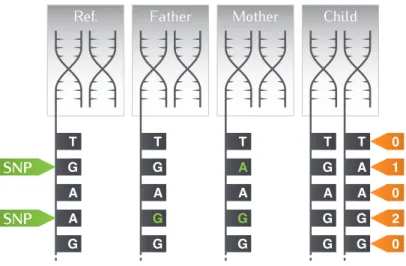
Figure 2.2 illustrates these ideas: the right-most part shows part of the dna inherited by a child from its two parents, by depicting a chromosome pair around five nucleotides; the two central parts show the corresponding dna of the corresponding chromosomes of its two parents; finally the left-most part shows the content of the corresponding wild-type chromosome of the reference population. In green, mutations are highlighted, yielding eventually the genotype of the child and its encoding in orange.
Note that sometimes that representation is not the exact one being used; one can indeed decide to code these values by using any specific allele as a reference (most of the time, the mutant allele is the one that is less frequent in a reference population).
2.3
Genome-wide associations studies
Snps have the potential to help identify the multiple genes associated with many phenotypes. Of course, snps generally do not directly cause an illness but they can help us to identify genomic regions potentially containing mutations causally affecting the biology of the studied phenotype and they could hence help us to evaluate the risk that someone will develop a disease. Identification of causal mutations will provide better diagnostic information that will allow for early diagnosis, prevention and better treatment of human diseases. In the following, we will indifferently use the word ”phenotype” to refer to the trait under study which can be a disease or any observable characteristic also called a trait (such as morphology, development, biochemical or physiological properties, behavior...). The phenotype can be qualitative (e.g., disease status) or quantitative (e.g., treatment response status). Analyzing dna can help to understand what is happening beyond the genetic code, in other words, what are the underlying molecular mechanisms leading to a given phenotype. Genome-wide association studies are designed for that purpose. However, as those genetic variations are transmitted through generations, they also are directly related to ancestry and family relations among individuals.
Mother Father Ref. Child T G A A G T G A G G T A A G G T G A G G T A A G G SNP SNP 0 1 0 2 0
Figure 2.2 Mother and father chromosomes dna differ from reference dna at one locus (a/g mutation, in green); the
mother in addition differs at a second locus (g/a mutation in green). The child’s genotype is obtained by combining these variations resulting from the inherited chromosome pair (in orange).
Unlike monogenic Mendelian diseases, a disease is said to be complex when multiple interacting genes and environmental factors are responsible for the phenotype. These complex diseases are not caused in a deterministic way by a single genetic mutation; rather they must have an intricate molecular architecture and may therefore be influenced by a potentially large number of genetic and environmental factors which may act in additive, complementary and/or more complex ways. Most of the time, in that case, it has been observed that each individual genetic variant only makes a very small contribution to the overall heritability of the disease. Since complex diseases are intrinsically related to the perturbation of a complex biological sub-system, this may explain the dispersed association among individual genetic variations and disease phenotype, as well as a rather high sensitivity to environmental factors. In addition to this dispersive effect, it may be the case that part of the heritability of genetic risks towards complex diseases can only be explained by conditional effects, i.e. effects which imply a conjunction of genetic and environmental factors. It might be the case that a multitude of such dispersed and/or conjunctive effects in the end is responsible of the fact that most of these complex diseases are not rare in the population.
When performing a genome-wide association study, the main questions we are trying to answer are the following:
• How many genetic variants are involved ?
• Where are these genetic variations located on the genome ? Do they appear in exons or introns ?
Which genes do these changes affect ?
• What is the type and biological consequence of each alteration ? Which allele is protective and which
one is causative ?
• What are the functional consequences of these changes ?
• how often such mutations occur (allele frequency, mutation rate) ? • Are these variants more important than environmental factors ?
• Are there any interactions between the genetic and environmental effects ?
• Can we infer the disease risk, or more generally predict a phenotype, based on genetic factors alone
Typically, to carry out such a study one disposes of a cohort of a few hundred to several thousand individuals, a fraction of them (typically about 50%) having a certain phenotype which are called cases, and the rest of them being individuals representative of the genetic variation in the studied population and who do not present the studied phenotype which are called controls. This is schematically represented at Figure 2.3.
FREQUENCY COMPARISONS
CASES CONTROLS
Figure 2.3 Overall principle of a genome-wide association study: step 1 (top) consists in collecting a cohort of cases
and controls (experiment design); step 2 (middle) consists in extracting DNA from the individuals and carrying out measurements to characterize their genetic variations (e.g. genotyping at snp loci); step 3 (bottom) consists in analyzing the resulting dataset so as to identify significant associations among groups of snps and phenotype and to determine risk prediction models (statistical inference).
2.3.1
Thanks to linkage disequilibrium
Advances in genotyping technologies allow for genome-wide association studies. In a short time, hundreds of thousands (and even more) snps spread over the whole genome can be genotyped for large sets of individuals at low cost. Denser genotyped variations over the whole genome should allow to detect causative dna regions even if the biologically causative mutation is not directly observed, indeed, those variants are known to be strongly correlated. Thus, the chances of finding an snp ”linked” with the causal one are highly increased (indirect association vs. direct association. See Figure 2.4).
Causal
mutation disequilibriumLinkage
(a) (b)
Figure 2.4 We talk about direct association (a) when the causal mutation is directly genotyped. On the other hand, if
only variations in ld with the causal mutation are genotyped then we talk about indirect association (b).
That “link” is also called the linkage disequilibrium (ld). It denotes the nonrandom association of alleles at two or more loci. One way of measuring ld between two variants is to compute a simple statistic for a
pair of snps. Doing so for each pair of snps will generate a matrix of values from which ld patterns can be deduced.
The International HapMap Project [The03] investigated ld patterns across the entire human genome. They started by gathering anonymized samples from four different populations: 90 Yoruba (30 parent-offspring trios) from Ibadan (Nigeria); 90 individuals (30 parent-offspring trios) of European ancestry from Utah, 45 unrelated Han Chinese from Beijing and 45 unrelated Japanese from Tokyo. Their findings pointed out that there exist hotspots of recombination in the genome which drive the observed ld patterns. They observed blocks of high ld separated by sharp breakdown of ld corresponding to hotspots.
Those blocks of high ld are also referred to as haplotype blocks. The term haplotype is a contraction of haploid genotype. Haplotypes are the combinations of alleles at different positions along the same chromo-some that are transmitted together. It may be much more informative to analyze them simultaneously instead of independently. These haplotypes have a particular structure which provides information on evolution history. According to the International HapMap Project, we now know that chromosomes are structured in many blocks, i.e., haplotype blocks within which there is a limited haplotype diversity (where little to no recombination events occured) separated by small regions of high haplotype diversity. This structure is population dependent.
Technically, the main benefit of those low haplotype diversity regions is that only a few markers need to be genotyped to capture the whole haplotype information. Selecting the minimal number of snps that uniquely identify common haplotypes is called haplotype tagging. That property has driven the current gwas in selecting the right amount of markers along the genome in order to capture a maximum of the variations present in the population under study. However, being focused on common variations, a direct (and maybe not so desirable) consequence is that the possible presence of rarer mutations may be missed and their potential implications underestimated.
To explain the notion of linkage disequilibrium, let us consider two snps, the first has alleles A and B, and the second has alleles C and D. In a given population, let us suppose that the marginal allele frequencies are fA, fB = 1 − fA, fC and fD = 1 − fC, respectively. We define a haplotype as being a
particular combination of the alleles of these two snps on one chromosome at variant sites and denote the haplotype (joint) frequencies as fAC, fBC, fAD and fBD.
A B Total
C fAC = fAfC+D fBC = fBfC−D fC
D fAD= fAfD−D fBD = fBfD+D fD
Total fA fB
Table 2.1 In this table, D represents the departure from the uncorrelated state in which the joint frequencies is equal
to the product of the marginal frequencies. When D is equal to 0 the two snps are said to be in linkage equilibrium (le).
The situation can be summarized in Table 2.1 where the standard coefficient D of LD between the two loci is defined by:
DAC= fAC− fAfC. (2.1)
Equation 2.1 expresses that the expected haplotype frequency in the absence of LD is the product of
the marginal frequencies. DAC represents the departure from the uncorrelated state. Simple algebraic
rearrangement shows that:
DAC= −DBC = −DAD= DBD. (2.2)
of one of the alleles. Also, the sign of D is sensitive to the allele code which can be chosen arbitrarily. To circumvent those two drawbacks, two derived LD statistics which both are frequency normalized and always positive are more commonly used:
|D0| = −DAC min(fAfC,fBfD) if DAC< 0, DAC min(fAfD,fBfC) if DAC> 0, (2.3)
|D0| ranges from 0 to 1, 0 means linkage equilibrium, a value of 1 corresponds to complete ld (the two
loci are not separated by recombination, i.e. at most three of the four possible haplotypes are present in the population) but does not necessary indicates that one locus can predict the other with high accuracy.
r2 = D
2 AC
fAfBfCfD
. (2.4)
The r2 is the squared Pearson correlation coefficient, a value of one corresponds to perfect ld for which
at most two haplotypes are possibly present. In other words, knowing the allele at one locus allows to predict the allele at the other one.
From these metrics, it is possible to compute a matrix of ld. Figure 2.5 shows an example of observable patterns in a small chromosome 1 region in the Hapmap ceu population. It allows to visually detect blocks of snps in high ld clearly separated by ld breakdown.
Figure 2.5 An example of ld pattern in the Hapmap ceu population, on chromosome 1 (67.68..68.18Mb) region. The
different pairwise values of D0 are represented by different intensity of red. We clearly see “triangles” of
higher ld depicting the haplotype block structure in that region.
2.4
GWAS : how ?
A genome-wide association study is driven by the following steps (see also Figure 2.3):
1. Choosing and collecting samples: maybe the most difficult part of a GWAS, collecting samples isn’t easy at all. Cases may sometimes be rare and for some diseases, getting dna samples is delicate. An accurate definition of the trait under study is required to minimize the heterogeneity of the underlying causal factors and increase the power of the study. Another major difficulty arises from matching case and control populations in order to avoid (or at least minimize) sample stratification.
2. Genotyping: using recent technologies allows now for genotyping massive amounts of markers at low cost. Genotyping arrays now provide up to one million common snps which currently approximately costs 400$ (and that cost will continue to decrease over time, while the number of variants assayed will increase). For that task, two main manufacturers (Affymetrix and Illumina) respectively provide hybridization-based and enzyme-based genotyping technology. In the end, these genotyping arrays allow to measure allele intensities at several locations in the genome from which genotypes can be
deduced. For further information concerning genotyping arrays, we refer the reader to [K+03] and
[S+06].
3. Quality controls: due to the previous steps, it is necessary to check the quality of the resulting data. Those quality control methods (qc) will be further discussed in Section 2.4.1.
4. Statistical analysis: there are two main approaches, the single-locus analysis where each variant is tested in turn and the multi-locus approaches where haplotypes, gene-gene (and possibly higher-order) interactions can be considered. Basically, this step consists in frequency or similarity comparisons between the cases and the controls. These tests are presented in Sections 2.4.2 and 2.4.3.
5. Replication: once some loci have been identified as being statistically associated to the studied phenotype, replication allows to validate or invalidate those results. The replication study is often carried by the use of a different genotyping platform, which may help to remove spurious associations due to technical artefacts.
2.4.1
Quality controls
Once the data have been collected and the genotypes assayed, we want to avoid confounding of signal with something that is not linked to the trait under study. Many quality control (qc) procedures exist to reduce the risk of false-positive and false-negative findings. Basically, those qc procedures can be based on samples or markers. In the following, the main qc procedures used in practice are discussed. For further reading we suggest the recently published tutorial from the genomics group of the eMERGE [T+11].
Sample-based QC
• Sample mix-ups and plating errors: it is possible that during the preparation, some samples are mixed
up on the plate. It can be messy and sometimes two or more samples are inverted on the array (usually composed of 96 wells). One way of detecting such errors is to check the sex recorded when collecting information about the samples and the one that can be estimated using the X chromosome. E.g., a female with a low heterozygosity rate across the X chromosome markers is probably a good indication of sample mix-up. Also, by mistake, if two samples are placed in the same well it will produce an excess of heterozygosity (on the other hand, low heterozygosity indicates inbreeding).
• Low-quality dna samples: quality and concentration of the collected dna may vary from one sample
to another, especially when the cases and the controls are not collected and extracted in the same place which can introduce spurious association. Even on the same plate, it is inevitable to observe variations in the quality and concentration, bad quality and/or low concentration samples often lead to failure of signal amplification causing genotypes to be uncallable which results in missing genotypes. In that case, individuals with an insufficient overall call rate should be removed from the study.
• Plate effects: it is also required to check if there are no differences in genotyping frequency between
plates. Especially in the situation where cases and controls are typed on different plates, such differences will cause confounding. A common practice is to evenly distribute cases and controls across plates. When it is not possible, a comparison of allele and/or genotype frequencies between one plate against the others will help identify significant differences and allow to discard samples from a study.
• Population stratification: one source of spurious associations is the presence of individuals coming
from different ancestral and demographic history. Especially when cases and controls strongly differ regarding these features. It has been clearly observed that many markers carry such an information and demographic information can thus be confounded with disease status. In order to avoid associating
that kind of markers to the disease, the first thing that can be done is to remove the outliers from the population under study. Most of the time, using principal component analysis and the addition of known and various ancestry (such as HapMap) genotypes allow for the identification of population structure and permit to confront the collected samples provenance informations to known populations. It has been observed that only two principal components are sufficient to separate clusters of different ancestry individuals. Another approach consists in calculating a genetic distance between pairs of individuals and using the resulting distance matrix to cluster the individuals. Similarly, duplicate and related samples can be identified using the same genetic distance; an abnormally small distance between a pair of individuals would indicate sample duplication and/or relatedness.
Marker-based QC
• Call-rate and Allele Frequency: unfortunately, genotyping platforms are not 100% reliable and could
cause some uncertainty for many reasons. When the genotype calling1 algorithm is not able to
determine the genotype at a given position for a given sample, this measurement is normally considered as missing. If a few genotypes are missing, it is not so problematic, since snps with missing values can be removed without loosing too much information and if the genotyping is dense enough we could hope that another snp in ld with the missing one has been correctly genotyped.
At each locus, for each sample, the genotyping technique measures the intensity of allele a and b. For all the individuals, each genotype can be summarized by a genotype cluster plot (Figure 2.6) which are used for the determination of genotypes. In other words, the analysis of allele intensities is used to determine the genotype at that given locus. Poor quality genotype cluster plots lead to poor confidence in genotype calling, which can lead to a missing genotype or calling errors. Many algorithms are used to this end, we refer the interested reader to [VSKZ09] for a detailed comparison of genotype calling algorithms, to [M+10] which highlights the potential inconsistencies between calling
algorithms that can impact downstream analyses and to [L+10] for a proposal of a statistic to evaluate the imputation reliability. Most of these calling algorithms outputs a confidence score for each snp, when that score is too low, the corresponding genotype is considered as missing.
Depending on the study, marker with an overall high missing rate should be removed from the study. Otherwise, they can be imputed by predicted values that are based on the observed genotypes at neighboring snps. To this end, softwares such as IMPUTE2 [HDM09] exists. Basically, the imputation process exploits the missing genotype surrounding ld structure and the associated known haplotypes to “guess” what would be the genotype. These algorithms relies on a reference haplotype panel (such as the HapMap samples).
Another common practice is to remove snps with a low minor allele frequency (maf). Such variables are difficult to study as they require large sample size to gain sufficient statistical power. However, [M+09] suggests that part of the missing heritability could be explained by such rare and recent
variations.
• Hardy-Weinberg Equilibrium: the Hardy-Weinberg equilibrium (HWE) principle states that genotype
frequencies at any locus are a simple function of allele frequencies (in the absence of migration, mutation, natural selection and assortative mating). In other words, at a given locus, where the alleles Aand B are observed, respectively, at frequencies fA= pand fB= q = 1−p, the following genotype
frequencies are expected:
fAA = p2, (2.5)
fBB = q2, (2.6)
fAB = 2pq. (2.7)
intensity (B) intensity (A) 0 1 2 1 2 BB AA AB
Figure 2.6 Genotype cluster plot: the green dots are clearly pointing out bb genotyped samples, the blue ones the
other homozygous and the orange ones the heterozygous. The remaining dark gray dots correspond to samples for which the genotype is difficult to determine.
Where fAA, fAB and fBB are the expected genotype frequencies for the homozygous wild,
heterozy-gous and homozyheterozy-gous mutant respectively. It has been observed that these expectations hold for most human populations and in practice, deviations from HWE can indicate inbreeding, population stratifi-cation and genotyping problems. A χ2 test between the expected frequencies and observed ones may
detect such deviations. But these deviations can also pinpoint association [NEW98], since deviations from HWE can be due to a deletion polymorphism or a segmental duplication that could be responsible for a phenotype. Thus, one must be careful before discarding loci based on that test.
2.4.2
Single-locus test of association
Suppose that we look at a particular SNP in two sub-groups of a population: cases (individuals affected by the disease under study) and controls (individuals not affected). We denote the number of individuals in the two sub-groups by ncase and ncont respectively. At that loci, let us say that we observe the 2 alleles: A,
B. Genotype counts can be summarized in a two-way contingency table, as illustrated in Table 2.2. Such a table can be analyzed using an observed-expected test statistic which has a χ2distribution with two degrees of freedom in order to detect whether there is any relationship, or association, between the genotype and the disease status.
AA AB BB Total
Cases a b c ncase
Controls d e f ncont
Total nAA= a + d nAB= b + e nBB= c + f n
Table 2.2 Full genotype table for a general genetic model : 2 × 3 table
Based on Table 2.2, the idea is to spot genotype significant differences between cases and controls. The main question is to find whether or not there is an association between the genotype (columns) and the phenotype (rows). In Table 2.2, there is no association when the proportion of each genotype remains the same regardless the disease status. These counts are said to be expected under the null hypothesis that there is no association.
follows: fAA = (a + d) n , (2.8) fAB = (b + e) n , (2.9) fBB = (c + f ) n , (2.10)
and from these frequencies, expected counts are derived, as shown in Table 2.3. It has to be noted that the total counts remain the same as in Table 2.2.
AA AB BB Total
Cases ncasefAA ncasefAB ncasefBB ncase
Controls ncontfAA ncontfAB ncontfBB ncont
Total a + d b + e c + f n
Table 2.3 Expected genotype counts
The idea is now to detect if there is a significant difference between the observed values (Table 2.2) and the expected ones under the independence hypothesis (Table 2.3). This can be achieved using the standard Pearson’s χ2 statistical test for independence of the rows and columns:
r X i=1 c X j=1 (Oij− Eij)2 Eij (2.11)
where Oij is the observed count and Eij is the expected count in the cell in row i and column j. If the null
hypothesis of no association is true, then the calculated test statistic approximately follows a χ2distribution
with (r − 1) × (c − 1) degrees of freedom (where r is the number of row variants and c is the number of column variants) i.e. in our case (r − 1) × (c − 1) = 2. This approximation can be used to obtain a p-value. A small p-value will suggest that there is association between the variables (genotype-phenotype) but the test will not indicate which are the cells (genotypes) in the contingency table that are the most associated. The χ2 p-value of an observation corresponds to its probability plus all the more extreme ones under the
null hypothesis (represented in green at Figure 2.7).
From those univariate tests, a p-value is assigned to each SNP, and thus a ranking of variables may be performed and a Manhattan plot (see Figure 2.8) is usually used to visualize the results. Spotting regions of interest is then a question of correct thresholding over the resulting p-values. Depending of the size of the spotted regions and on the genotyping density, it is often expected to see several variants for which the p-values are way under the significance level α.
One of the major issues at a genome-wide level is the multiple testing problem. Indeed, the larger the number of hypothesis tests, the larger is the probability of getting significant results due to chance. One way to correct for multiple testing is to adjust α (using methods like the Bonferroni, the ˇSid´ak or the Benjamini-Hochberg correction) in order to “control” the Type I error rate. Other methods exist such as
permutation based adjustments. Resampling can be performed exhaustively, leading to so-called exact tests (if the set of observations is small enough) or approximate test (otherwise), such as Monte Carlo simulations. These tests allow for an estimation of how often a random observation can be as extreme as the observed one.
As a recommendation for the χ2 test, the sample size should be such that no cells in the table have an
expected count of less than one and no more then 20% of the cells should have an expected count of less than five. If samples are small, then Fisher’s exact test can be used at the price of a higher computational cost. The exact p-value can be calculated by considering all the tables with the same row and column totals
un-likely observations most likely observations P robability possible observations observation p-value
Figure 2.7 The curve represents the probability of every observed outcome under the null hypothesis. The p-value is
the probability of the observation plus all the more extreme ones, represented by the green area.
Figure 2.8 A Manhattan plot is used to identify regions where p-values are under the significance level. Each point
represent a snp (at its chromosomal position, chromosome by chromosome) and its associated χ2p-value.
The red dotted line represents a significance level of 10−5 = 0.00001, p-values under that threshold
may pinpoint causal regions. On the CD1 Crohn’s disease related dataset (see Chapter 6), among others,
noticeable regions are found on chromosomes 1, 5 and 16 (which have been confirmed as being involved in the disease).